| Issue |
A&A
Volume 665, September 2022
|
|
|---|---|---|
| Article Number | A94 | |
| Number of page(s) | 25 | |
| Section | Interstellar and circumstellar matter | |
| DOI | https://doi.org/10.1051/0004-6361/202142305 | |
| Published online | 19 September 2022 | |
Inverted level populations of hydrogen atoms in ionized gas
1
Shanghai Astronomical Observatory, Chinese Academy of Sciences,
80 Nandan Road,
Shanghai,
200030, PR China
e-mail: This email address is being protected from spambots. You need JavaScript enabled to view it.
; This email address is being protected from spambots. You need JavaScript enabled to view it.
2
Research Center for Intelligent Computing Platforms, Zhejiang Laboratory,
Hangzhou
311100, PR China
3
School of Physical Science and Technology, Guangxi University,
Nanning
530004, PR China
4
Department of Astronomy, University of Science and technology of China,
Hefei
230026, PR China
5
Physics Department, Guangzhou University,
Guangzhou
510006, PR China
Received:
24
September
2021
Accepted:
22
May
2022
Abstract
Context. Level population inversion of hydrogen atoms in ionized gas may lead to stimulated emission of hydrogen recombination lines, and the level populations can in turn be affected by powerful stimulated emissions.
Aims. In this work the interaction of the radiation fields and the level population inversion of hydrogen atoms is studied. The effect of the stimulated emissions on the line profiles is also investigated.
Methods. Our previous nl-model for calculating level populations of hydrogen atoms and hydrogen recombination lines is improved. The effects of line and continuum radiation fields on the level populations are considered in the improved model. By using this method the properties of simulated hydrogen recombination lines and level populations are used in analyses.
Results. The simulations show that hydrogen radio recombination lines are often emitted from the energy level with an inverted population. The widths of Hnα lines can be significantly narrowed by strong stimulated emissions to be even less than 10 km s−1. The amplification of hydrogen recombination lines is more affected by the line optical depth than by the total optical depth. The influence of stimulated emission on the estimates of electron temperature and density of ionized gas is evaluated. We find that comparing multiple line-to-continuum ratios is a reliable method for estimating the electron temperature, while the effectiveness of the estimation of electron density is determined by the relative significance of stimulated emission.
Key words: line: profiles / methods: numerical / stars: massive / HII regions / radio lines: ISM
© F.-Y. Zhu et al. 2022
 Open Access article, published by EDP Sciences, under the terms of the Creative Commons Attribution License (https://creativecommons.org/licenses/by/4.0), which permits unrestricted use, distribution, and reproduction in any medium, provided the original work is properly cited.
This article is published in open access under the Subscribe-to-Open model. This email address is being protected from spambots. You need JavaScript enabled to view it. to support open access publication.
1 Introduction
Ionized gas, which is mainly composed of ionized hydrogen and electrons, is a common phase of the interstellar medium (ISM). This gas is usually formed by the extreme-ultraviolet (hv ≥ 13.6 eV) photons emitted from massive stars, post-asymptotic giant branch (post-AGB) stars, supernovas (SNs), or active galactic nuclei (AGNs). Star formation activities and the evolution of massive stars in molecular clouds can be studied from observations toward ionized gas caused by massive stars (Kim et al. 2017; Liu et al. 2021). Hydrogen radio recombination lines (RRLs) and continuum emissions can be used to derive the electron temperature and density of ionized gas (Wood & Churchwell 1989). These basic properties of ionized gas are helpful to determine the effective temperature and the mass of the ionizing star, the chemical abundances of the ionized gas, and the conditions of the ambient medium (Peimbert 1979; Shaver et al. 1983; Afflerbach et al. 1994; Zhu et al. 2019).
The line-to-continuum ratio at centimeter and millimeter wavelengths is a common tool used to estimate the electron temperature of the ionized gas with an assumption of local thermo-dynamic equilibrium (LTE) conditions (Churchwell & Walmsley 1975; Shaver et al. 1983). However, in actual situations, the level populations of hydrogen atoms do not perfectly satisfy the LTE assumption (Sejnowski & Hjellming 1969; Brocklehurst 1970). This could lead to a significant difference between the estimated and the actual electron temperatures (Sorochenko & Borodzich 1966; Höglund & Mezger 1965; Gordon & Sorochenko 2002).
The excitation states of hydrogen can be classified into the cases of population inversion, overheating, thermalization, and overcooling (Strelnitski et al. 1996). In the cases of population inversion and overheating, line emission can be increased by stimulated emission and become higher than that expected under the LTE assumption. When the hydrogen recombination lines are strongly amplified due to the inverted level populations, line masers occur. The first hydrogen recombination line maser source discovered was the young stellar object (YSO) MWC 349A (Martin-Pintado et al. 1989); hydrogen recombination line masers were then also found in other sources (Cox et al. 1995; Jiménez-Serra et al. 2011; Aleman et al. 2018). The first extra-galactic hydrogen recombination line maser was discovered in NGC 253 (Bâez-Rubio et al. 2018). For some H II regions stimulated emissions are also important, although the line masers cannot be identified (Afflerbach et al. 1994). For these cases, the estimation method under the LTE assumption is not applicable.
In order to improve the accuracy of the estimation, the non-LTE conditions of the level populations of hydrogen atoms have been considered in some previous works (Afflerbach et al. 1994; Bâez-Rubio et al. 2013). The accuracy of the departure coefficients of the level populations of hydrogen from the populations under LTE conditions is important for the estimation of electron temperature. The departure coefficients have been studied for more than 50 yr (Sejnowski & Hjellming 1969). In early works, the departure coefficients were calculated via the n-model in which only the transitions between different energy levels were considered (Brocklehurst 1970; Walmsley 1990). The nl-model, which included angular momentum changing transitions, was used in Storey & Hummer (1995), and the calculated values were then applied to specifying the conditions necessary for hydrogen recombination line masers (Strelnitski et al. 1996). Prozesky & Smits (2018) improved the nl-model with the consideration of the effect of the continuum radiation. By using the departure coefficients calculated by the nl-model without the effect of radiation fields, we provided a method for estimating the electron temperature and density of ionized gas from hydrogen RRLs in Zhu et al. (2019). However, the accuracy of this method has not been checked for H II regions with high electron density (ne ≥ 104 cm−3) and high emission measure (EM), where the departure coefficients could be significantly affected by line and continuum radiation (Prozesky & Smits 2018).
The departure coefficients and the intensities of hydrogen recombination lines were recently calculated under maser conditions by Prozesky & Smits (2020). Both the effects of radio free-free continuum and hydrogen recombination line radiation on the level populations were considered in their work. However, in this model the hydrogen recombination lines are all assumed to have a box profile with the same amplitude as the Doppler profile. This simple assumption cannot reproduce the actual line profiles. Since the optical depth of the hydrogen recombination line is clearly affected by the line width, the fluxes of the hydrogen recombination lines should also be influenced. The broadening of the hydrogen recombination line is related to the velocity field, electron temperature, and density (Peters et al. 2012). Conversely, line masers can also influence the widths of the hydrogen recombination lines (Thum et al. 1995). Moreover, the spectral simulation code CLOUDY (Ferland et al. 2017) can also treat hydrogen recombination lines under maser conditions. The radiation fields and realistic line profiles are included in this code (Guzmán et al. 2019). However, the effects of the radiation fields and line profiles on hydrogen level populations have not been explored with CLOUDY in previous works.
In this work we improve the nl-model produced in Zhu et al. (2019) with the effects of the radiation fields due to the hydrogen recombination lines and the continuum emission. The effects of the line and continuum radiation fields on the departure coefficients are studied. The relation between the line profile and the emissions of the hydrogen recombination lines is also investigated. The performance of the estimation method to derive the electron temperature from the line-to-continuum ratio under LTE assumptions for ionized gas with a series of properties is presented. Finally, we test the reliability of the estimated properties of H II regions by using hydrogen recombination lines and the continuum emissions in multiple wavebands.
2 Method
2.1 The calculation of departure coefficients in Case B
The accuracy of calculations of level populations and departure coefficients of hydrogen atoms is important for the simulation of hydrogen recombination lines and continuum emission. Level population equations consists of a series of linear equations (Salgado et al. 2017; Prozesky & Smits 2018), and can be written in matrix form as
 (1)
(1)
where the elements of matrix A and vector y refer to the processes of different transitions from or to the state nl. The vector b is composed of the partial departure coefficients (bn1). Then, by solving the matrix equation, bn1 can be obtained. An iterative method for evaluating bn1 is described in Brocklehurst (1971), and is also used in Storey & Hummer (1995) and Salgado et al. (2017). In that method, the values of bn1 with the same principal quantum number n are solved simultaneously with a n × n matrix, while the partial departure coefficients with the other principal quantum numbers are treated as known quantities in the equations. Prozesky & Smits (2018) used a direct solver to calculate the departure coefficients, and provide an error estimate of the quality of the results derived from the norms of the matrix and vectors as
 (2)
(2)
This value can be used to estimate the convergence of the departure coefficients.
In our previous work, an algorithm to calculate the departure coefficients (bn) was used in the case when the radiation field does not have a significant effect on level populations (Case B) (Zhu et al. 2019). The iterative method was used in the algorithm, and the calculations were terminated if the largest difference of departure coefficients between two iterations  is less than 1 × 10⁻⁶, where t means the sequence number of iterations. This criterion could be too simple. In this work we directly solve the matrix equation. The error estimate is ϵ ~ 3 × 10⁻⁵ in all the cases. The convergence should be reached with this value of the error estimate.
However, as mentioned in Zhu et al. (2019), the resulting departure coefficients of our method are closer to the results provided in Storey & Hummer (1995) than those in Prozesky & Smits (2018), although the rates of transition processes we used are similar to those in Prozesky & Smits (2018). More checks were done, and they confirm the reliability of our results. The details are presented in Appendix A.
The amplification coefficients (βn,n+1) with the principal quantum number n calculated by this algorithm for different electron densities (ne) are presented in Fig. 1. The amplification coefficients represent the departure of the level population ratios from their LTE values (Strelnitski et al. 1996; Prozesky & Smits 2018). Shown in Fig. 1, the result is similar to those calculated in the previous works in the literature (Storey & Hummer 1995; Strelnitski et al. 1996). The ranges of principal quantum number n in the cases of population inversion (βn,n+1 < 0), overheating (0 < βn,n+1 < 1), thermalization (βn,n+1 = 1), and overcooling (βn,n+1 > 1) are shown, while the locations and the widths of these ranges changing with ne are also presented. The center of the valley of βn,n+1 is closer to the left side of the low principal quantum number with high electron density ne, while the width and depth of the valley rises with decreasing ne. The result shows that population inversion is a common phenomenon for hydrogen radio recombination lines. This motivates us to study in detail the significance of the stimulation effect due to population inversion under different conditions. The level populations of hydrogen atoms could be influenced when stimulated emission is important. So in this work, the effects of the line and continuum radiation fields on the level populations and departure coefficients are both added to the new algorithm.
2.2 Departure coefficients calculated with the effects of line and continuum radiation fields
Hydrogen recombination lines, continuum emission, and the “one-layer” assumption are used when calculating departure coefficients. Ionized gas is homogeneous and isothermal. In the calculation the initial conditions include electron temperature (Te), electron density (ne), and emission measure (EM). In the beginning the departure coefficients are derived by directly solving the matrix equation of level populations with no radiation fields. In the second step these values of departure coefficients are used to calculate the mean intensities of incident radiation fields due to line and continuum emissions. Then the departure coefficients are calculated with the intensities of the incident radiation fields, while the new values of the intensities are estimated from the new departure coefficients. This process is operated iteratively until the values of the departure coefficients converge.
Because the radiation fields and the calculated departure coefficients are inter-related, the error estimate derived from the solution of the matrix equation cannot directly be used to evaluate the convergence. We replace bt (the vector b composed of bnl in the current step t) with bt−1 in the last step t − 1 to calculate the error estimate, and terminate the calculation when the two error estimates calculated with bt and bt−1 are approximately equal. This is a reasonable stopping criterion since the values of bt and bt – 1 should be very close when the iterative calculation has converged. It is also found that the  is always lower than 10−9 when the calculation converges.
In addition, the mean intensity of line and continuum radiation fields (Jv) need to be calculated in order to evaluate the effects of the radiation fields on the level populations. However, for a cloud of ionized gas, Jv should be treated nonlocally in principle with different quantities in every volume element.
This would make the calculations very time consuming, so following Kegel (1979), we assume that the electron temperature, density, absorption coefficient (κν), and source function (S′v) are all homogeneous, and then the mean intensity of the incident radiation field is
 (3)
(3)
where τv is the optical depth at the frequency v and  is also called the escape probability. However, the box line profile as a further simplification used in Kegel (1979), Koeppen & Kegel (1980), and Röllig et al. (1999) is not assumed in this work. As defined in Hummer & Storey (1987), the mean radiation field is
 (4)
(4)
where ϕv is the line profile function (Peters et al. 2012). In the calculation of departure coefficients, we replace the term Jv in Eq. (5) of Prozesky & Smits (2018) with J. Moreover, for the transitions about n = 1, the Lyman transitions are still assumed to be optically thick, and the collisional excitations from n = 1 and n = 2 states are also ignored, as in Zhu et al. (2019).
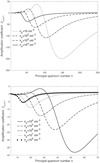 |
Fig. 1 Value of βn,n+1 varies with principal quantum number n for Te = 10 000 K and different electron densities ne. |
2.3 Radiative transfer
In this work only the hydrogen recombination lines and the continuum emission are considered to be the radiation fields that could affect the level populations of hydrogen atoms. The radiation from sources out of the ionized gas such as the stellar radiation field and the cosmic microwave background, and the emission from dust are not included since the influences of these emissions are generally weak (Prozesky & Smits 2018). In addition, the gas temperature is assumed to be equal to the electron temperature. For uniform ionized gas, the continuum absorption coefficient κv is derived by Oster (1961) and Gordon & Sorochenko (2002) with the Rayleigh-Jeans approximation (hv ≪ kTe), which is evaluated numerically as
![Mathematical equation: ${\kappa _{v,C}} = 9.770 \times {10^{ - 3}}{{{n_e}{n_i}} \over {{v^2}T_e^{1.5}}}\left[ {17.72 + \ln {{T_e^{1.5}} \over v}} \right],$](/articles/aa/full_html/2022/09/aa42305-21/aa42305-21-eq8.png) (5)
(5)
where ne and ni are respectively the number densities of electrons and ions in units of cm−3, Te is the electron temperature in units of K, v is the frequency in Hz, and κv,C is in units of cm−1. The continuum optical depth is τvC = κv,CD with the line-of-sight (LOS) depth D. Then the free-free continuum emissivity jv,C and the intensity of the continuum emission JvC are
 (6)
(6)
and
 (7)
(7)
where Bv(Te) is the intensity of a blackbody at temperature Te and frequency v. The line absorption coefficient at frequency v for the transition from lower level n to higher level m including the processes of absorption and stimulated emission is
 (8)
(8)
where Nn is the total number density of hydrogen atoms with the principal quantum number n, Nnl is the number density of those of level nl, and l is the angular momentum number. Similarly, Bnm and Bnlmv are the Einstein coefficients for absorption and stimulated emissions of the corresponding transitions, and they are derived from the spontaneous Einstein coefficients Amn and Aml′ni (Brocklehurst 1971; Prozesky & Smits 2020). The parameter ϕν is the line profile function. Following Gordon & Sorochenko (2002) and Peters et al. (2012), when calculating the profiles of the hydrogen recombination lines, the line profile function is calculated by considering the thermal, velocity field, and pressure broadenings. The population of hydrogen atoms in level n under the LTE assumption is (Peters et al. 2012)
 (9)
(9)
where k is the Boltzmann constant, h the Planck constant, En is the energy of level n below the continuum, and me is the electron mass. The emission coefficient of a hydrogen recombination line is
 (10)
(10)
where  is the line absorption coefficient calculated with the LTE level populations. The source function Sν is provided by
 (11)
(11)
where ßn,m is the amplification coefficient given by
 (12)
(12)
The total intensity and the observed line intensity at the frequency ν for a uniform H II region are respectively given by
 (13)
(13)
and
 (14)
(14)
where the total optical depth is τv = κνD. The total absorption coefficient is κν = κvC + κvL, and this value may be negative if the contribution of the stimulated emission is more than that of absorption. The line absorption coefficient can also be presented as  ..
..
In this paper, the results of a series of simulations are presented. The effect of the radiation field on level populations of hydrogen atoms is considered in almost all of the simulations except for those especially indicated. On the contrary, the effect of the velocity field is only included in some simulations in Sect. 3.2. In addition, the one-layer model is used in all the simulations, except where a “two-layer” model is included in the calculations in Sect. 3.6.
3 Results and discussions
3.1 Variations in departure and amplification coefficients with radiation field
In order to assess the effect of radiation fields on the departure coefficients bn and the amplification coefficients βn,n+1, we compared the values of bn and βn,n+1 calculated by using the non-LTE method with and without the effect of the line and continuum radiation fields. The results in the conditions of different electron temperatures and densities were analyzed, and the radiation fields were found to have a similar effect on bn and βn,n+1. As an example, one case with electron temperature Te = 10 000 K and electron density ne = 106 cm−3 is presented. The comparisons of bn and βn,n+1 are presented in the top and middle panels of Fig. 2. By adjusting the value of EM, the intensity of the radiation field is changed in the calculations. It is clear that the distortions ofbn and βn,n+1 increase with the intensity of the radiation field.
The saturation intensity (Js) is introduced by Strelnitski et al. (1996) as a criterion compared with the mean intensity of the radiation fields (Jv) to estimate the degree of saturation. In the bottom panel of Fig. 2 the comparison of the mean intensities of the radiation fields and the saturation intensity is shown. The saturation intensity first decreases and then increases with the principal quantum number n. This occurs because the decay rate is dominated by the spontaneous decay at low energy level n and by the collisional decay at high energy level n, and the former decreases with the energy level while the latter increases. From the results shown in Fig. 2, it is unsurprising that the saturation intensity can be a rough criterion to evaluate the influence of the radiation fields on bn and βn,n+1. For the case of EM = 1.0 × 1010 cm−6 pc, Jv is lower than Js for all the Hnα lines, and the distortion of bn and βn,n+1 are also very slight. The mean intensities Jv corresponding to EM = 3.0 × 10¹⁰ and 5.0 × 1010 cm−6 pc are higher than Js for a range of Hnα lines, and the values of bn and βn,n+1 at the corresponding principal quantum numbers n are changed significantly, but this criterion is still not very accurate. On the two sides of the valley of βn,n+1, the values of bn and βn,n+1 can be changed significantly even if Jv is lower than Js. The stimulated emission triggered by the saturated masing line from n + 1 to n strongly increase the population of the lower level n and decreases that of the upper level n + 1 . This effect can decrease the population inversion between levels n and n + 1 . However, it can also increase the population inversions between the levels n − 1 and n, and between n + 1 and n + 2 if the stimulated emissions of the adjacent lines of n + 2 to n + 1 and n to n − 1 are relatively weak (Strelnitski et al. 1996; Prozesky & Smits 2020). Since the radiation field is saturated (Jv > Js) in the range of n ~ 20–50 corresponding to the valley of βn,n+1 at the conditions of EM = 3.0 × 10¹⁰ and 5.0 × 1010 cm−6 pc, the population inversion is weakened in the center and strengthened on the two sides of the valley of βn,n+1.
The total optical depths (τv) and the total intensities (Iv) including the line and continuum intensities calculated with different EMs are presented in Fig. 3. The black lines represent the values derived from the departure coefficients bn calculated without the radiation fields, while the red lines represent the values calculated with the effect of radiation fields. The distortions of bn and βn,n+1 shown in Fig. 2 are clearly amplified in the intensities and optical depths displayed in Fig. 3. The intensities of the stimulated lines could be overestimated considerably in the center of the masing range and underestimated on the two sides if the radiation fields are not included in the calculations of bn and βn,n+1. This is not surprising because of the effect of radiation fields on the population inversion mentioned above. In addition, the effect of the radiation fields causes the valley of the optical depth to be shallower and wider. For the conditions of EM = 3.0 × 10¹⁰ and 5.0 × 1010 cm−6 pc, the ranges of τv < −1 are wider when the radiation fields are considered. In the literature, a typical maser is thought to occur if the total optical depth τv < −1 (Strelnitski et al. 1996; Thum et al. 1998; Prozesky & Smits 2020). Strelnitski et al. (1996) suggested that saturated higher frequency masing lines could “attract” adjacent lower frequency lines to exhibit masing, and this is confirmed by the numerical calculation in Prozesky & Smits (2020). Our results show that it is also possible for saturated lower frequency masing lines to attract adjacent higher frequency lines to be masing.
In Fig. 4 the frequency-integrated intensities of the Hnα lines and the total optical depths τv calculated with the LTE assumption are compared to those calculated without the LTE assumption. In this case, as an example, the electron density ne is 3.0 × 106 cm−3, and EM is assumed to be 1011 cm−6 pc. As displayed in the top panel, the stimulated emission could raise the line intensity by several magnitudes more than the LTE intensity, even with a thick continuum optical depth (τvC > 1). This difference of line intensities is kept until βn,n+1 and bn increase to be 1 at high energy level n.
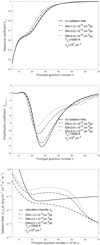 |
Fig. 2 Level populations of hydrogen atoms affected by radiation fields. The departure coefficients bn varying with principal quantum number n affected by different radiation fields are plotted in the top panel. The amplification coefficients βn,n+1 influenced by different radiation fields are presented in the middle panel. The corresponding intensities of mean radiation field ∫ Jvϕvdv and the saturation intensity Js are shown in the bottom panel. The electron temperature is Te = 10 000 K, and the electron density is ne = 106 cm−3. |
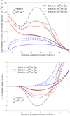 |
Fig. 3 Influence of radiation fields on hydrogen RRLs. The total intensities at the frequencies of the Hnα line calculated with different EMs are plotted in the top panel. The total optical depths at the frequencies of the Hnα lines are presented in the bottom panel. The solid, dashed, and dash-dotted lines represent the values for EM = 1.0 × 10¹⁰, 3.0 × 10¹⁰, and 5.0 × 1010 cm−6 pc, respectively. The black lines represent the values calculated without the effect of radiation fields on level populations, and the red lines the values calculated with radiation fields. The blue lines show the values of the continuum emissions. |
3.2 Effects of electron temperature and velocity field on βn,n+1 and line emissions
By affecting the line optical depth, the line profile has an important influence on the line emission when the stimulated emission is great. So it is necessary for us to study the effect of line profiles on the departure coefficients and recombination lines. If the velocity field is mainly caused by microturbulence, the line profile function ϕv of the hydrogen recombination line is generally a Voigt profile, a convolution of the Doppler and Lorentz profiles. This line profile function is determined by Te, ne, and the root mean square σv of the microturbulent velocity field (Peters et al. 2012). In the top panel of Fig. 5, the ratios of the frequency-integrated line intensities ∫ Iv,Ldv to the intensities calculated under the LTE and optically thin assumptions  with different turbulence velocity fields are presented. The optically thin assumption is commonly used in the analyses of observations, and leads to the LTE value being overestimated when the actual optical depths of continuum and line are high (Kim et al. 2017; De Pree et al. 2020). In this case the electron temperature and density are Te = 10000 K and ne = 106 cm−3, respectively, while EM is 3 × 1010 cm−6 pc. The root mean squares of the velocity field σv are adjusted to be 0, 10, and 20 km s−1. From the recent observations for the H40α line toward ultra-compact H II regions (Liu et al. 2021), the assumptions of the velocity fields are appropriate. It is clear in the top panel of Fig. 5 that the intensity of the hydrogen recombination line is significantly affected by the line profile function. The greater broadening due to the stronger turbulence would widen the line profile so that the absolute value of the optical depth is reduced. This weakens the stimulated emissions, and reduces the distortions of βn,n+1 from the values calculated without the radiation fields, as presented in the bottom panel of Fig. 5.
The electron temperature Te is also an important condition that affects the properties of the hydrogen recombination lines. The width of the line profile function is influenced by temperature. The continuum absorption coefficients and the LTE line absorption coefficients both decrease with increasing temperature. The level populations, the departure coefficients and the amplification coefficients are also affected by the electron temperature. The amplification coefficients βn,n+1 for different temperatures are presented in the bottom panel of Fig. 6. In the calculations the electron temperatures are assumed to be 8000, 10 000, and 12 000 K, and the velocity field of ionized gas is not considered. The other conditions are indicated in the panel. The line absorption coefficient κv,L is a decisive factor in the strength of stimulated emission. It is proportional to the product of βn,n+1 and  . As shown in the bottom panel, the negative value of βn,n+1 is more significant when the temperature is higher, but the value of
  decreases with increasing temperature. Since the absolute value of the product of βn,n+1 and κv,L decreases with increasing electron temperature, the contribution of simulated emission to the hydrogen recombination line emission increases with decreasing temperature. This trend is clearly shown in the top panel of Fig. 6.
 |
Fig. 4 Effect of stimulation emission on hydrogen RRLs. The frequency-integrated intensities of the Hnα line calculated under LTE assumption (solid line) and using non-LTE method without and with the effect of radiation field on departure coefficients (dashed and dash-dotted line) vs. principal quantum number n are plotted in the top panel. The total optical depths at the frequencies of the Hnα lines are presented in the bottom panel. The red vertical lines indicate the positions of the continuum optical depth τvC = 1 and 5. |
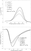 |
Fig. 5 Effects of different velocity fields on hydrogen RRLs. In the top panel the ratios of the frequency-integrated line intensities ∫ Iv,Ldv to the intensities calculated under the LTE and optically thin assumptions |

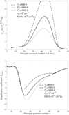 |
Fig. 6 Hydrogen RRLs affected by different electron temperatures. In the top panel the ratios of the frequency-integrated line intensities ∫ Iv,Ldv to the intensities |

3.3 Widths of masing Hnα lines
In addition to the effect of the velocity field of ionized gas, the widths of hydrogen recombination lines are mainly determined by thermal and pressure broadenings when the optical depth is thin and the stimulated emissions are not important (Gordon & Sorochenko 2002). When line masers occur, the line widths can be narrowed because the amplification of intensity at the line center is much greater than that at the sides, due to the approximately exponential increase in stimulated emissions with the absolute value of the optical depth (Strelnitski et al. 1996).
The variations in the widths of the Hnα lines are plotted in Fig. 7, which shows the maser effect on the widths of Hnα lines. The change in the line widths with n also indicates the influence of pressure broadening. Pressure broadening can increase the widths of hydrogen recombination lines. The effect of pressure broadening is important when electron density ne is high, and it increases with n for Hnα lines. The effect of the line maser on line width can be neglected when the pressure broadening is very large due to high values of ne and n. However, the maser effect can still significantly decrease the widths of Hnα lines when the influence of pressure broadening is low. The results in Fig. 7 show that the maser effect may reduce the full width at half maximum (FWHM) of the Hnα line profile by several km s−1 . For a H II region with a low equilibrium temperature of Te ~ 5000 K, the FWHM of the Hnα line may even be lower than 10 km s−1 . In addition, although only the narrow Hnα line widths with n < 70 are shown in Fig. 7, the widths of Hnα lines with high n will also be narrowed by the maser effect when the electron density becomes lower than 105 cm−3. Comparing the results presented in the top three panels of this figure, it is clear that the maser effect increases with EM. According to our calculations, the reduction in hydrogen recombination line widths due to line masers is significant (>2 km s−1) only if the EM is higher than 3.0 × 107 cm−6 pc. This range of EMs corresponds to the conditions of hyper-compact, ultra-compact, and compact H II regions (de la Fuente et al. 2020b).
Some cases of hydrogen recombination line maser have been detected in previous observations (Martin-Pintado et al. 1989; Cox et al. 1995; Jiménez-Serra et al. 2011; Aleman et al. 2018). In the case of MWC349, comparing the widths of the H26α, H27α, H36α, and H40α lines in Table 2 of Thum et al. (1995), the ~ 11 km s-1 widths of the red and blue components of the H26α and H27α lines are narrowed by the stimulation effect. The difference between the widths of the broad component of the H30α and H38β lines also shows the effect of stimulated emission. In addition, many H II regions with narrow hydrogen recombination lines have been discovered (Lockman 1989; Planesas et al. 1991; Anderson et al. 2011; Chen et al. 2020). Although “cool” nebulae with low electron temperatures because of high metal abundances can lead to these narrow lines (Shaver 1970; Shaver et al. 1979), the maser effect is also a natural explanation for these phenomena.
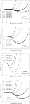 |
Fig. 7 Variations in the Hnα line widths with principal quantum number n. The FWHMs presented in the top three panels are calculated with Te = 10 000 K, and the FWHM in the bottom panel is calculated with Te = 5000 K. The values of the EMs are the same as in the calculation results shown in the same panel, while the values of the corresponding LOS depth D are different since the values of ne are different. |
3.4 Line optical depth leading to observable line masers
Goldberg (1966) pointed out that the hydrogen recombination line intensity, increased by the strong stimulated emission, with a negative line optical depth τvL can be significantly higher than its LTE value, even if the total optical depth τv is still positive. However, Strelnitski et al. (1996) claimed that a total optical depth much lower than −1 is necessary to produce an observable maser amplification.
From our calculation of the case mentioned in Sect. 3.1 and shown in the top panel of Fig. 4, we find that the ratio of the non-LTE Hnα line intensity to the LTE value with high energy level n > 48 and positive τv is even higher than that with considerably negative optical depth τv < −1 at low energy level n < 48. The profiles of the H30α, H50α, and H70α lines are presented in Fig. 8 along with the LTE profiles of these lines. At the H30α line center, τv = −3.84 and τv,L = -4.13. The peak brightness temperature Tb of the H30α line is higher than the Tb under the LTE assumption. For the center of the H50α line, τv,C = 7.73 is thick, τv = 0.10 is positive, and the line optical depth τv,L = −7.63 is significantly lower than −1. The brightness temperature Tb of the continuum emission is 9995.6 K because of the very thick continuum optical depth, and the line center of the H50α line even reaches 9.9 × 10⁴ K. The LTE line center is only 4.4 K, which is several orders lower than the non-LTE line strength. The width (FWHM) of the H50α optical depth profile function is 22.9 km s−1, while the FWHM of the H50α line profile is only 13.0 km s−1 because the maser effect is important. On the other hand, due to the relatively thick optical depth, the FWHM of the H50α line will be 36.6 km s−1 if the LTE assumption is used. In addition, for the center of the H70a line, τv = 65.9 and τv,L = 0.32. The level population is overheating, and the amplification coefficient is β70,71 = 0.14. The temperature Tb at the line center is 292 K. On the contrary, the emission at the center of H70α will be negligible due to the very high optical depths if the LTE assumption is used.
The H II regions B2 and G2 in W49A observed by De Pree et al. (2020) show very high EM > 5 × 109 cm−6 pc. Although the corresponding continuum optical depth should be higher than 18, the H92a line in these sources can still be detected. This cannot be explained under the LTE assumption, whereas inversion or overheating of the level population should exist. Under non-LTE conditions, the stimulated emission produced by a population inversion could make the corresponding hydrogen recombination line detectable even if the continuum optical depth is very thick.
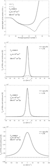 |
Fig. 8 Relation between the line optical depth and the maser amplification. The total and line optical depths vs. the energy level n is displayed in the top panel. The brightness temperature Tb of the H30α, H50α, and H70α line profiles and the continuum is presented in the top middle, bottom middle, and bottom panels, respectively. |
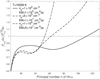 |
Fig. 9 Ratios of non-LTE frequency-integrated line intensities to LTE values |

3.5 Significance of stimulated emissions
In the preceding sections we show results only for hyper-compact H II regions. However, the stimulated emissions still show significant influence in more classical H II regions. We use the classification of H II regions provided by de la Fuente et al. (2020b) in the subsequent analyses of the importance of stimulated emissions.
The ratios of non-LTE Hnα line intensities to LTE values  for the typical conditions of ultra-compact, compact, and extended H II regions are plotted in Fig. 9. The ratio decreases quickly with decreasing n when the principal quantum number n is lower than 20. Then after a small decline in the range of n ≈ 20–40, the ratio increases monotonically when the n is higher. When the principal quantum number n is low, the line and continuum optical depths are very small. Then the ratio is approximately equal to the departure coefficient at the upper level. When the optical depths increase with n, stimulation has a gradually more important influence on the Hnα line intensity. Moreover, the significance of stimulation is greatly influenced by EM. For ultra-compact H II regions, the Hnα line intensities in the range of n > 60 under non-LTE conditions are higher than those under LTE conditions; the non-LTE values are lower than the LTE values for extended H II regions until n exceeds 105.
As mentioned above, the ratio of non-LTE Hnα line intensity to the LTE value increases with n if the small decline in the range of n ≈ 20–40 is ignored. We define as the biggest n with which the non-LTE Hnα line intensity is more than 15% lower than the one in LTE. And  is defined as the smallest n with which the non-LTE Hnα line intensity is more than 15% higher than the LTE value. Then the Hnα lines in the range between
  and
and  can be treated under the LTE assumption with an error <15%.
The values of  and
and  at different ne and EMs for Te = 5000 and 10 000 K are listed in Table 1. Temperatures of Te = 10 000 K are typical for H II regions, and the values for Te = 5000 K can display the conditions in low-temperature H II regions. The upper limit of the Lyman continuum photon production rate
  is assumed to be 1.5 × 1050 s−1 corresponding to the rate of a young massive star cluster (Nguyen-Luong et al. 2017). For a spherical and uniform H II region,
  can be calculated from Te, ne, and radius r = D/2 by using Eq. (A4) in de la Fuente et al. (2020b). Conversely, the r and EM for given Te and ne can be estimated from
  . Considering that H II regions might be not spherical, the upper limit of EM is assumed to be 2 times of the value of EM calculated from the upper limit of
  with given Te and ne under the assumption of spherical H II regions. Furthermore, the lower limit of EM is calculated from the
  = 1044 s−1 corresponding to the value of an ~8 M⊙ massive star (Diaz-Miller et al. 1998).
As is shown in Table 1, the range of n between  and
and  gradually becomes narrow with the increase in EM. The Hnα lines in the centimeter waveband (60 ≤ n ≤ 129) are often used to derive the LTE temperature
  under the LTE assumption as a close estimate of the actual Te (Shaver et al. 1983; Wilson et al. 2015). In our calculations, the LTE approximation for most of the centimeter Hnα lines is appropriate when EM is lower than 106 cm−6 pc. On the contrary, in the cases of ultra-and hyper-compact H II regions with EM > 5 × 107 cm−6 pc, the deviation from the LTE approximation is commonly significant for the centimeter Hnα lines. Some of the millimeter Hnα lines (28 ≤ n < 60) may be useful to accurately estimate the actual Te under the LTE approximation for ultra-compact H II regions, but the suitable range of n is often narrow and changes strongly with EM. So a precise estimate of EM is necessary to determine the range of Hnα lines suitable for the LTE approximation. For hyper-compact H II regions, the suitable range of n changes greatly with Te and ne. Even if the EM is known, no Hnα lines can be assured to be appropriate for the LTE approximation before Te and ne are obtained.
3.6 Effect of population inversion in extended HII regions around ultra-compact HII regions
The results presented in Table 1 seem to suggest that the contribution from stimulated emission to the centimeter Hnα lines is relatively weak and lower than 15% if EM < 106 cm−6 pc. However, as for the case of the extended H II region (ne = 102 cm−3 and EM = 105 cm−6 pc) plotted in Fig. 9, there could still be an approximately 10% difference between the non-LTE and LTE line intensities. If Te and ne are lower, the difference will be bigger. Furthermore, the stimulation effect could be much strengthened if the low-EM H II region has strong emission in the background.
Some ultra-compact H II regions have been found located near extended free-free emission (EE; de la Fuente et al. 2020a,b). de la Fuente et al. (2020a) suggest that EE seems to be common in ultra-compact HII regions. The EM of an EE is typically 104–105 cm−6 pc, and the ne is ~102 cm−3 (de la Fuente et al. 2020b). However, since large-scale structures of ionized gas are easy to miss in interferometric observations (Wood & Churchwell 1989), the contribution to hydrogen recombination lines from the extended component are probably overlooked. Two cases including an ultra-compact H II region + EE, and a hyper-compact H II region + EE are calculated. The Te is 10 000 K in both cases. The values of ne are 106, 105, and 102 cm−3 for the hyper-compact regions, ultra-compact H II regions, and the EE, respectively, and the corresponding EMs are 108, 5 × 10⁷, and 105 cm−6 pc. The high-density region and the extended region are assumed to have the same LOS velocity. Since the high-density H II region is embraced by EE, the EE is treated as a component in front of the high-density H II region. The hydrogen recombination lines passing through both the high-density and extended regions are studied.
The profiles of the H110α line in the three cases are shown in Fig. 10. The line profiles calculated respectively from hyper- and ultra-compact H II regions and EE as a single component are also plotted. Compared with the line profiles from single components, it is clear that the population inversion in the EE can significantly strengthen the line emission from ultra- or hyper-compact HII regions. Especially in the case of hyper-compact H II regions + EE, the part of the line emission contributed from the hyper-compact H II region is very broad. Its broad profile can be regarded as the baseline. If so, the part attributed to the stimulated emissions from the EE will be mistakenly treated as the line emission mainly emitted from the hyper-compact H II region. In addition, the line widths are also influenced by the EE. The widths (FWHMs) of the H110a line just emitted from the hyper- and ultra-compact H II regions are 870 and 92 km s−1, respectively. Then they become much narrower, 23 and 49 km s−1 after the line emission passes through the EE.
When observing the Hnα lines from the hyper- and ultracompact H II regions, it is meaningful to evaluate the contamination from the EE. Compared with the line emissions just emitted from hyper- and ultra-compact H II regions, whether the contribution of the stimulated emissions from the EE needs to be considered is determined by the line optical depth τv,L of the EE and the ratio of Iv,L/Iv,L of the line and continuum emissions before passing through the EE. For hyper-compact H II regions with high electron density and EM that lead to very low Iv,L/Iv,C the stimulated emission from EE may increase the peak Tb of the Hnα line by more than 15% when n > 85. Even if the EM of the EE is only 104 cm−6 pc, the stimulated emission is still non-negligible when n > 100. For ultra-compact H II regions embraced by the EE with EM = 105 cm−6 pc, the stimulated emission needs to be considered when n > 100.
Range of the Hnα lines suitable for the LTE approximation.
3.7 Estimation of the properties of ionized gas including the effect of stimulated emissions
3.7.1 Uncertainty of estimated electron temperature under the LTE assumption
The LTE temperature (T*), which is the electron temperature estimated from the line-to-continuum ratios under the LTE and optically thin assumptions, has been commonly used to evaluate the actual electron temperature of ionized gas. However, the LTE temperature T* may be significantly different from the actual electron temperature Te (Afflerbach et al. 1994; Gordon & Sorochenko 2002). In Figs. 11 and 12, the variations in the LTE temperature T* with the values of EM and ne of the ionized gas are presented. These LTE temperatures are estimated from the ratios of the frequency-integrated intensities of a series of Hnα lines to the continuum intensities at the corresponding frequencies. We calculated the case for an actual electron temperature Te = 10 000 K only. From the results displayed in Figs. 11 and 12, the deviation of the LTE temperature from the actual temperature is mainly determined by the departure coefficient bn when the continuum optical depth is very thin. If the departure coefficient bn is close to 1 due to high electron density or high energy level n, the LTE temperature will be relatively accurate. When the continuum optical depth increases, the values of T* could be lower due to the increasing effects of the stimulated emission on the Hnα line emitted from the energy level n without the LTE condition. If the LTE condition is approximately satisfied in the energy levels n and n + 1, the LTE temperature estimated from the Hnα line will increase with the continuum optical depth. By using these hydrogen radio recombination lines, the actual electron temperature can hardly be evaluated from the LTE temperature if the continuum optical depth is τv,C > 0.1 and the electron density ne is unknown.
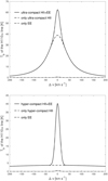 |
Fig. 10 Line profiles of the H110α line for two cases. The result in the case of ultra-compact HII region + EE is presented in the top panel, and that of hyper-compact H II region + EE is shown in the bottom panel. The values of ne are 106, 105, and 102 cm−3 for the hyper-compact, ultracompact, and extended H II regions, respectively, and the corresponding EMs are 108, 5 × 10⁷, and 105 cm−6 pc. The electron temperature is Te = 10 000 K. |
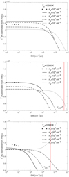 |
Fig. 11 LTE temperature estimated from H30α, H40α, and H60α lines with the continuum emission vs. EM for Te = 10 000 K and different ne. The red vertical lines indicate the value of EM corresponding to the continuum optical depth τv,C = 1. |
3.7.2 Deriving properties of ionized gas with line-to-continuum ratios of multiple RRLs under non-LTE conditions
Using multiple line-to-continuum ratios at different wavebands may be a good method for estimating the electron temperature and density of ionized gas, which had been used for the ultracompact HII region G29.96-0.02 with the departure coefficients calculated using the n-model (Afflerbach et al. 1994). However, just being successfully applied to one case does not prove that this method will work well in other situations. To study the applicability of this method, we performed a systematic analysis.
As observable parameters, the line-to-continuum ratios of the a lines of hydrogen and continuum intensities at given frequencies can be used to derive Te, ne, and EM, with the method using multiple line-to-continuum ratios under non-LTE conditions. However, systematic errors or deviation in this method need to be checked. Line-to-continuum ratios for every a line of hydrogen and continuum intensities at given frequencies can be derived based on our non-LTE model, with given values of Te, ne, and EM for one ionized region. Uncertainties in the observations, including flux calibration and white noise, should be considered during such calculation. From the simulated line-to-continuum ratios with observational uncertainties, the estimated Te, ne, and EM can be compared with the input parameters. The reliability of the estimation method is then assessed.
We give an example of the results of this calculation including the information of H30α, H40α, and H60α line intensities to the continuum intensities at the corresponding frequencies with the method using multiple line-to-continuum ratios. In addition, the continuum intensity at the frequency of 99.023 GHz is also used. This can significantly improve the estimation accuracy.
For one case of an ionized region, we first calculate the frequency-integrated line intensities and the continuum emission intensities at the corresponding frequencies for the given values of Te, ne, and EM, based on our model. Three line-to-continuum ratios are then derived. After that, a group of four random numbers are generated from the normal distribution based on the calculated values of the three line-to-continuum ratios and the 99.023 GHz continuum intensity. The calculated values are taken as the means of the normal distributions. We assume the uncertainty in the ratio observations to be 3 and 10%, and the uncertainty in the continuum intensity observation to be 3%. These uncertainties are used as the standard deviations. The four random numbers in one group are used to simulate the four quantities measured in observations. Then values of Te, ne, and EM are adjusted until the resulting line-to-continuum ratios and the 99.023 GHz continuum intensity fit the simulated values. The least-squares method is used in the fitting process. After the process mentioned above is repeated many times, a series of best fit values of Te, ne, and EM are then derived from many groups of four random numbers. These best fit values create the distributions of the estimated Te, ne, and EM. Finally, the mean values and the uncertainties of these estimated quantities are calculated from the distributions.
In Table 2, the resulting estimates of Te for hyper-compact H II regions are given. The mean values and the corresponding 1c uncertainties are presented with the assumed uncertainties (σ/µ) of the line-to-continuum ratios of 3 and 10%; the uncertainty of the continuum emission at 99.023 GHz is always assumed to be 3%. According to the results shown in the table, the mean values of the estimated electron temperatures Te are always close to the actual temperature Te = 10 000 K. In addition, the relative uncertainties of the estimated temperatures are mostly lower than 8 and 2% for 10 and 3% uncertainties of the line-to-continuum ratios, respectively.
In Table 3, the estimated Te for the cases of ultra-compact, compact, and extended H II regions are given. The hydrogen recombination lines used in the estimation method are the H40α, H80α, and H120α lines. The 99.023 GHz continuum intensity is still used in these cases. The estimated values of Te for these relatively low-density H II regions are still very accurate, as in the cases for hyper-compact HII regions. This suggests that a believable estimate of electron temperature can be obtained by using this estimation method.
The LTE temperatures T* estimated with a single line-to-continuum ratio under the LTE assumption for the corresponding cases of H II regions are also given in Tables 2 and 3. The uncertainty of T* is approximately proportional to 0.87 times the uncertainties of the corresponding line-to-continuum ratio because the LTE temperature is about  (Gordon & Sorochenko 2002). In general, the deviation between the LTE temperature and the actual temperature is mainly affected by the difference between the frequency-integrated line intensities under non-LTE and LTE conditions. If the non-LTE Hnα line intensity is significantly different (>15%) from that under LTE, the LTE approximation should not be used. Additionally, the systematic deviation of the non-LTE method using multiple line-to-continuum ratios is very slight in estimating electron temperature. This is different from the LTE method. Therefore, even if the difference between the line intensities under non-LTE and LTE conditions is not great (<15%), the method using multiple line-to-continuum ratios is still preferable when a high precision of estimated electron temperature is required.
Moreover, the estimated values of the electron density ne and the EM are also displayed in Tables 2 and 3. The value of the optically thin continuum emission is very sensitive to EM but relatively insensitive to Te and ne. This makes the estimated values of EM very accurate if the continuum optical depth is thin. In addition, by using the multiple line-to-continuum ratios, the estimated value of the EM can still be accurate even if the continuum optical depth is thick (τv,C ~ 10), although the uncertainty of the estimated EM may be a little bigger. The estimation of the electron density ne is sensitive to the departures of line-to-continuum ratios from their LTE values. This departure increases with the EM and decreases with the electron density ne. The ratios of the frequency-integrated line intensity (∫Iv,Ldv) to the line intensity calculated under the LTE assumption  for the Hnα lines are also listed in Tables 2 and 3. These ratios are useful to evaluate the importance of stimulated emission. When stimulated emission is not important, the line-to-continuum ratios are close to their values in LTE. These values can lead to inaccurate estimates of ne since the line-to-continuum ratio is not sensitive to ne under LTE conditions. On the contrary, when stimulated emission is important, the line-to-continuum ratios significantly depart from the LTE values. Then the estimated values of ne can be very close to the actual values. In the case of ne = 105 cm−3 and EM = 109 cm−6 pc, the estimated ne values using different combinations of Hnα lines are given in Tables 2 and 3. Comparing the different estimated ne, it shows that choosing hydrogen recombination lines with larger amounts of stimulated emission helps to accurately estimate electron density.
In Tables B.1–B.3 the total optical depths τv at the centers of the hydrogen recombination lines for different temperatures, densities, and EMs are listed. The line optical depths τv,L for different properties are given in Tables B.4–B.6. The optical depths can help us to speculate whether or which Hnα lines show maser emission from the known properties of ionized gas. The line-to-continuum ratios are presented in Tables B.7-B.9. These values are useful to estimate the electron temperature, density, and EM of ionized gas by using multiple line-to-continuum ratios.
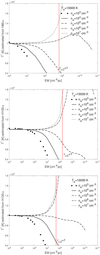 |
Fig. 12 LTE temperature estimated from H80α, H100α, and H120α lines with the continuum emission vs. EM for Te = 10 000 K and different ne. The red vertical lines indicate the value of EM corresponding to the continuum optical depth τv,C = 1. |
Estimated values and standard deviations of Te, ne, and EM for hyper-compact H II regions.
Estimated values and standard deviations of Te, ne, and EM for ultra-compact, compact, and extended H II regions.
4 Summary and conclusions
In this work the departure coefficients bn and the amplification coefficient βn,m+1 are calculated by using an nl-model with the effects of line and continuum radiation. The effects of radiation fields, electron temperature, and density, and the velocity field on the departure coefficients, the amplification coefficients, and the Hnα lines are investigated. The results show that the population inversion (βn,n+1 < 0) often occurs in hydrogen atoms in the ionized gas that emits hydrogen RRLs. The effect of stimulated emission on the Hnα line widths is also studied, and we find the powerful stimulation effect can significantly narrow the line widths of the Hnα lines, even down to less than 10 km s−1 under certain conditions, although this effect is not important for the line widths when the EM < 3 × 107 cm−6 pc. We assess the reliability of the method of using multiple hydrogen line-to-continuum ratios to estimate Te, ne, and EM of the ionized gas. We find this method is helpful to obtain the accurate values of Te and EM. The accuracy of the estimated ne is determined by the stimulation effect on the Hnα lines. The other details of our conclusions are summarized as follows:
The saturation intensity Js introduced by Strelnitski et al. (1996) is a rough criterion for evaluating the influence of the radiation fields on bn and (βn,n+1< 0) but may underestimate the influence especially for the high energy level n. Not only could the saturated higher frequency masing lines cause adjacent lower frequency lines to exhibit masing, but the saturated lower frequency masing lines may also lead to adjacent higher frequency masing lines.
The Hnα line emissions could be overestimated considerably if the radiation fields are not considered in calculating bn and βn,n+1< 0. Strong radiation fields could broaden the range of the population inversion < 0 in the principal quantum number n.
The stimulation effect of the hydrogen recombination lines can be weakened by violent velocity fields. Steep velocity gradients can lead to considerable broadening of the line profile that reduces the absolute value of the negative optical depth. The narrower line profile function due to lower electron temperatures can increase the stimulation effect.
The maser effect of the Hnα lines is mainly determined by the line optical depth, and can occur with considerably negative line optical depth even if the total optical depth τv > 0. In addition, the overheating and inversion of the populations can also produce amplification of the Hnα lines, although the total optical depth and the continuum optical depth are both very thick.
For uniform H II regions without strong background radio emission, most of the centimeter Hnα lines are appropriate for the LTE approximation when EM < 106 cm−6 pc. However, when there is strong background emission (e.g., a hyper- or ultra-compact H II region), stimulated emission could also be important for the centimeter Hnα lines even if EM ≤ 105 cm−6 pc.
The electron temperature estimated using a hydrogen RRL to free-free continuum ratio under the LTE assumption can be more than 50% different from the actual electron temperature.
In these conclusions, the influence of powerful radiation fields on level populations and hydrogen RRLs, the variation of stimulated emission with line width, and the deviation from the LTE approximation for RRLs are shown. They are helpful to estimate the significance of non-LTE conditions in observations of RRLs.
Acknowledgements
The authors thank the referee, Dr. A. Roy, and an anonymous referee for their constructive comments and detailed inspections to significantly improve the quality of the manuscript. The work is supported by the National Key R&D Program of China (No. 2017YFA0402604), the National Science Foundation of China No. 12003055, No. U1931104, and No. 11590782, China Postdoctoral Science Foundation No. 2020M671267, and Shanghai Post-doctoral Excellence Program No. 2018261. This work is also supported by the international partnership program of Chinese Academy of Sciences through Grant No. 114231KYSB20200009, the Strategic Priority Research Program of Chinese Academy of Sciences, Grant No. XDB41000000, and Key Research Project of Zhejiang Lab (No. 2021PE0AC03).
Appendix A Comparison of calculated departure coefficients with results in the literature
Our nl-model introduced in Zhu et al. (2019) with the Case B assumption contains the transition processes including radiative recombination (Burgess 1965), spontaneous emission (Brockle-hurst 1971), collisional excitations and de-excitations, collisional ionization, three-body recombination (Vriens & Smeets 1980), and angular momentum changing collisions (Pengelly & Seaton 1964; Guzman et al. 2016). The methods of calculating the rate coefficients of these processes are similar to those used in Prozesky & Smits (2018). In the previous work, we used the iterative method to calculate the departure coefficients. The n-model was solved first under the assumption of bnl = bn, and the nl-model was used to calculate bn and bni with n less than the critical level ncrit (Hummer & Storey 1987; Storey & Hummer 1995; Salgado et al. 2017). However, it was found that our results are closer to those in Storey & Hummer (1995) than to the values in Prozesky & Smits (2018), although the rate coefficients of bound-bound collisional transitions used in Storey & Hummer (1995) are different. In this work we replaced the iterative method with a direct solver, as done by Prozesky & Smits (2018) with error estimates ϵ ~ 3 × 10⁻⁵, but we find our results are still consistent with those in Storey & Hummer (1995) after the stopping criterion was improved.
As an example, the values of bn, bnl, and ßn,n+1 for Te = 104 K and ne = 105 cm−3 calculated by our model are compared with those provided by Storey & Hummer (1995) and Prozesky & Smits (2018) in Fig. A.1. The values of the departure coefficients in the tables provided by Storey & Hummer (1995) and Prozesky & Smits (2018) have four significant digits. This leads to the zigzags in the ßn n+1 lines in the bottom panel. The differences in amplification coefficients ßn,n+1 and partial departure coefficients between Storey & Hummer (1995) and Prozesky & Smits (2018) are not non-neglibile. It is clear that our results are consistent with those in Storey & Hummer (1995) since the small difference can be explained by the different rate coefficients of collisional excitations and de-excitations. Although the cause leading to the difference from the values of Prozesky & Smits (2018) is still unknown, we suggest that the departure coefficients calculated by us and Storey & Hummer (1995) are more accurate. And our nl-model should be reliable.
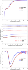 |
Fig. A.1. Departure coefficients bn, partial departure coefficients bnl, and amplification coefficients ßn,n+1 calculated by our model (current paper), Storey & Hummer (1995)(SH95), and Prozesky & Smits (2018) (PS18) are compared. The electron temperature Te is 104 K, and the electron number density is ne = 105 cm−3. |
Appendix B Tables of total optical depths, line optical depths, and line-to-continuum ratios
The values of τv and τv,L at the centers of the hydrogen recombination lines for different temperatures, densities, and EMs are listed in Tables B.1-B.6. The line-to-continuum ratios are given in Tables B.7-B.9.
Total optical depth τv at the center of the Hnα line as functions of electron density ne and EM.
Total optical depth τv at the center of the Hnα line as functions of electron density ne and EM.
Total optical depth τv at the center of the Hnα line as functions of electron density ne and EM.
Line optical depth τv,L at the center of the Hnα line as functions of electron density ne and EM.
Line optical depth τv,L at the center of the Hnα line as functions of electron density ne and EM.
Line optical depth τv,L at the center of the Hnα line as functions of electron density ne and EM.
Line-to-continuum ratios ∫Iv,Ldv/Iv,C [Hz] of the Hnα lines as functions of electron density ne and EM.
Line-to-continuum ratios ∫Iv,Ldv/Iv,C [Hz] of the Hnα lines as functions of electron density ne and EM.
Line-to-continuum ratios ∫Iv,Ldv/Iv,C [Hz] of the Hnα lines as functions of electron density ne and EM.
References
- Afflerbach, A., Churchwell, E., Hofner, P., & Kurtz, S. 1994, ApJ, 437, 697 [NASA ADS] [CrossRef] [Google Scholar]
- Aleman, I., Exter, K., Ueta, T., et al. 2018, MNRAS, 477, 4499 [NASA ADS] [CrossRef] [Google Scholar]
- Anderson, L. D., Bania, T. M., Balser, D. S., & Rood, R. T. 2011, ApJS, 194, 32 [NASA ADS] [CrossRef] [Google Scholar]
- Arthur, S. J., & Hoare, M. G. 2006, ApJS, 165, 283 [NASA ADS] [CrossRef] [Google Scholar]
- Báez-Rubio, A., Martín-Pintado, J., Thum, C., & Planesas, P. 2013, A&A, 553, A45 [NASA ADS] [CrossRef] [EDP Sciences] [Google Scholar]
- Báez-Rubio, A., Martín-Pintado, J., Rico-Villas, F., & Jiménez-Serra, I. 2018, ApJ, 867, L6 [CrossRef] [Google Scholar]
- Bodenheimer, P., Tenorio-Tagle, G., & York, H. W. 1979, ApJ, 233, 85 [NASA ADS] [CrossRef] [Google Scholar]
- Brocklehurst, M. 1970, MNRAS, 148, 417 [NASA ADS] [CrossRef] [Google Scholar]
- Brocklehurst, M. 1971, MNRAS, 153, 471 [Google Scholar]
- Burgess, A. 1965, MmRAS, 69, 1 [Google Scholar]
- Chen, H.-Y., Chen, X., Wang, J.-Z., Shen, Z.-Q., & Yang, K. 2020, ApJS, 248, 3 [NASA ADS] [CrossRef] [Google Scholar]
- Churchwell, E., & Walmsley, C. M. 1975, A&A, 38, 451 [NASA ADS] [Google Scholar]
- Cox, P., Martín-Pintado, J., Bachiller, R., et al. 1995, A&A, 295, L39 [NASA ADS] [Google Scholar]
- de la Fuente, E., Porras, A., Trinidad, M. A., et al. 2020a, MNRAS, 492, 895 [NASA ADS] [CrossRef] [Google Scholar]
- de la Fuente, E., Tafoya, D., Trinidad, M. A., Porras, A., & Nigoche-Netro, A. 2020b, MNRAS, 497, 4436 [NASA ADS] [CrossRef] [Google Scholar]
- De Pree, C. G., Wilner, D. J., Goss, W. M., Welch, W. J., & McGrath, E. 2000, ApJ, 540, 308 [NASA ADS] [CrossRef] [Google Scholar]
- De Pree, C. G., Wilner, D. J., Kristensen, L. E., et al. 2020, AJ, 160, 234 [Google Scholar]
- Diaz-Miller, R. I., Franco, J., & Shore, S. N. 1998, ApJ, 501, 192 [CrossRef] [Google Scholar]
- Ferland, G. J., Chatzikos, M., Guzmán, F., et al. 2017, Rev. Mex. Astron. Astrofis., 53, 385 [NASA ADS] [Google Scholar]
- Gaetz, T. J., & Salpeter, E. E. 1983, ApJS, 52, 155 [NASA ADS] [CrossRef] [Google Scholar]
- Goldberg, L. 1966, ApJ, 144, 1225 [NASA ADS] [CrossRef] [Google Scholar]
- Gordon, M. A., & Sorochenko, R. L. 2002, Radio Recombination Lines (Berlin: Springer) [CrossRef] [Google Scholar]
- Gordon, M. A., & Walmsley, C. M. 1990, ApJ, 365, 606 [CrossRef] [Google Scholar]
- Guzmán, F., Badnell, N. R., Williams, R. J. R., et al. 2016, MNRAS, 459, 3498 [CrossRef] [Google Scholar]
- Guzmán, F., Chatzikos, M., van Hoof, P. A. M., et al. 2019, MNRAS, 486, 1003 [CrossRef] [Google Scholar]
- Höglund, B., & Mezger, P. G. 1965, Science, 150, 339 [CrossRef] [Google Scholar]
- Hummer, D. G., & Storey, P. J. 1987, MNRAS, 224, 801 [NASA ADS] [CrossRef] [Google Scholar]
- Jiménez-Serra, I., Martín-Pintado, J., Báez-Rubio, A., Patel, N., & Thum, C. 2011, ApJ, 732, L27 [CrossRef] [Google Scholar]
- Kegel, W. H. 1979, A&AS, 38, 131 [NASA ADS] [Google Scholar]
- Keto, E. R., Zhang, Q., & Kurtz, S. 2008, ApJ, 672, 423 [NASA ADS] [CrossRef] [Google Scholar]
- Kim, W.-J., Wyrowski, F., Urquhart, J. S., Menten, K. M., & Csengeri, T. 2017, A&A, 602, A37 [NASA ADS] [CrossRef] [EDP Sciences] [Google Scholar]
- Koeppen, J., & Kegel, W. H. 1980, A&AS, 42, 59 [NASA ADS] [Google Scholar]
- Kurtz, S., Churchwell, E., & Wood, D. O. S. 1994, ApJS, 91, 659 [Google Scholar]
- Lockman, F. J. 1989, ApJS, 71, 469 [Google Scholar]
- Liu, H.-L., Liu, T., Evans, N. J., et al. 2021, MNRAS, 505, 2801 [NASA ADS] [CrossRef] [Google Scholar]
- Mac Low, M.-M., van Buren, D., Wood, D. O. S., & Churchwell, E. 1991, ApJ, 369, 395 [NASA ADS] [CrossRef] [Google Scholar]
- Martín-Pintado, J., Bachiller, R., Thum, C., & Walmsley, C. M. 1989, A&A, 215, L13 [Google Scholar]
- Murchikova, L., Murphy, E. J., Lis, D. C., et al. 2020, ApJ, 903, 29 [NASA ADS] [CrossRef] [Google Scholar]
- Nguyen-Luong, Q., Anderson, L. D., Motte, F., et al. 2017, ApJ, 844, 25 [NASA ADS] [CrossRef] [Google Scholar]
- Oster, L. 1961, RvMP, 33, 525 [NASA ADS] [Google Scholar]
- Peimber, M. 1979, IAU Symp. 84, 307 [Google Scholar]
- Pengelly, R. M., & Seaton, M. F. 1964, MNRAS, 127, 165 [NASA ADS] [CrossRef] [Google Scholar]
- Peters, T., Longmore, S. N., & Dullemond, C. P. 2012 MNRAS, 425, 2352 [NASA ADS] [CrossRef] [Google Scholar]
- Planesas, P., Gómez-González, J., Rodríguez, L. F., & Cantó, J. 1991, Rev. Mex. Astron. Astrofis., 22, 19 [Google Scholar]
- Prozesky, A., & Smits, D. P. 2018, MNRAS, 478, 2766 [NASA ADS] [CrossRef] [Google Scholar]
- Prozesky, A., & Smits, D. P. 2020, MNRAS, 491, 2536 [NASA ADS] [Google Scholar]
- Röllig, M., Kegel, W. H., Mauersberger, R., & Doerr, C. 1999, A&A, 343, 939 [Google Scholar]
- Salgado, F., Morabito, L. K., Oonk, J. B. R., et al. 2017, ApJ, 837, 141 [Google Scholar]
- Sejnowski, T. J., & Hjellming, R. M. 1969, ApJ, 156, 915 [NASA ADS] [CrossRef] [Google Scholar]
- Scoville, N., & Murchikova, L. 2013, ApJ, 779, 75 [CrossRef] [Google Scholar]
- Shaver, P. A. 1970, ApL, 5, 167 [NASA ADS] [Google Scholar]
- Shaver, P. A., McGee, R. X., & Pottasch, S. R. 1979, Nature, 280, 476 [CrossRef] [Google Scholar]
- Shaver, P. A., McGee, R. X., Newton, L. M., Danks, A. C., & Pottasch, S. R. 1983, MNRAS, 204, 53 [NASA ADS] [CrossRef] [Google Scholar]
- Sorochenko, R. L., & Borodzich, E. V. 1966, Sov. Phys.- Dokl., 10, 588 [NASA ADS] [Google Scholar]
- Spitzer, L. 1978, Physical Processes in the Interstellar Medium (New York: Wiley-Interscience), 333 [Google Scholar]
- Storey, P. J., & Hummer, D. G. 1995, MNRAS, 272, 41 [NASA ADS] [CrossRef] [Google Scholar]
- Strelnitski, V. S., Ponomarev, V., & Smith, H. A. 1996, ApJ, 470, 1118 [NASA ADS] [CrossRef] [Google Scholar]
- Tenorio-Tagle, G. 1979, A&A, 71, 59 [NASA ADS] [Google Scholar]
- Thum, C., Strelnitski, V. S., Martín-Pintado, J., Matthews, H. E., & Smith, H. A. 1995, A&A, 300, 843 [NASA ADS] [Google Scholar]
- Thum, C., Martn-Pintado, J., Quirrenbach, A., & Matthews, H. E. 1998, A&A, 333, L63 [NASA ADS] [Google Scholar]
- Thum, C., Neri, R., Báez-Bubio, & Krips, M. 2013, A&A, 556, 129 [Google Scholar]
- Vriens, L., & Smeets, A. H. M. 1980, Phys. Rev. A, 22, 940 [NASA ADS] [CrossRef] [Google Scholar]
- Walmsley, C. M. 1990, A&AS, 82, 201 [NASA ADS] [Google Scholar]
- Wilson, T. L., Bania, T. M., & Balser, D. S. 2015, ApJ, 812, 45 [NASA ADS] [CrossRef] [Google Scholar]
- Wood, D. O. S., & Churchwell, E. 1989, ApJS, 69, 831 [Google Scholar]
- Zhu, F.-Y., Zhu, Q.-F., Wang, J.-Z., & Zhang, J.-S. 2019, ApJ, 881, 14 [NASA ADS] [CrossRef] [Google Scholar]
All Tables
Estimated values and standard deviations of Te, ne, and EM for hyper-compact H II regions.
Estimated values and standard deviations of Te, ne, and EM for ultra-compact, compact, and extended H II regions.
Total optical depth τv at the center of the Hnα line as functions of electron density ne and EM.
Total optical depth τv at the center of the Hnα line as functions of electron density ne and EM.
Total optical depth τv at the center of the Hnα line as functions of electron density ne and EM.
Line optical depth τv,L at the center of the Hnα line as functions of electron density ne and EM.
Line optical depth τv,L at the center of the Hnα line as functions of electron density ne and EM.
Line optical depth τv,L at the center of the Hnα line as functions of electron density ne and EM.
Line-to-continuum ratios ∫Iv,Ldv/Iv,C [Hz] of the Hnα lines as functions of electron density ne and EM.
Line-to-continuum ratios ∫Iv,Ldv/Iv,C [Hz] of the Hnα lines as functions of electron density ne and EM.
Line-to-continuum ratios ∫Iv,Ldv/Iv,C [Hz] of the Hnα lines as functions of electron density ne and EM.
All Figures
|
Fig. 1 Value of βn,n+1 varies with principal quantum number n for Te = 10 000 K and different electron densities ne. |
| In the text | |
|
Fig. 2 Level populations of hydrogen atoms affected by radiation fields. The departure coefficients bn varying with principal quantum number n affected by different radiation fields are plotted in the top panel. The amplification coefficients βn,n+1 influenced by different radiation fields are presented in the middle panel. The corresponding intensities of mean radiation field ∫ Jvϕvdv and the saturation intensity Js are shown in the bottom panel. The electron temperature is Te = 10 000 K, and the electron density is ne = 106 cm−3. |
| In the text | |
|
Fig. 3 Influence of radiation fields on hydrogen RRLs. The total intensities at the frequencies of the Hnα line calculated with different EMs are plotted in the top panel. The total optical depths at the frequencies of the Hnα lines are presented in the bottom panel. The solid, dashed, and dash-dotted lines represent the values for EM = 1.0 × 10¹⁰, 3.0 × 10¹⁰, and 5.0 × 1010 cm−6 pc, respectively. The black lines represent the values calculated without the effect of radiation fields on level populations, and the red lines the values calculated with radiation fields. The blue lines show the values of the continuum emissions. |
| In the text | |
|
Fig. 4 Effect of stimulation emission on hydrogen RRLs. The frequency-integrated intensities of the Hnα line calculated under LTE assumption (solid line) and using non-LTE method without and with the effect of radiation field on departure coefficients (dashed and dash-dotted line) vs. principal quantum number n are plotted in the top panel. The total optical depths at the frequencies of the Hnα lines are presented in the bottom panel. The red vertical lines indicate the positions of the continuum optical depth τvC = 1 and 5. |
| In the text | |
|
Fig. 5 Effects of different velocity fields on hydrogen RRLs. In the top panel the ratios of the frequency-integrated line intensities ∫ Iv,Ldv to the intensities calculated under the LTE and optically thin assumptions |
| In the text | |
|
Fig. 6 Hydrogen RRLs affected by different electron temperatures. In the top panel the ratios of the frequency-integrated line intensities ∫ Iv,Ldv to the intensities |
| In the text | |
|
Fig. 7 Variations in the Hnα line widths with principal quantum number n. The FWHMs presented in the top three panels are calculated with Te = 10 000 K, and the FWHM in the bottom panel is calculated with Te = 5000 K. The values of the EMs are the same as in the calculation results shown in the same panel, while the values of the corresponding LOS depth D are different since the values of ne are different. |
| In the text | |
|
Fig. 8 Relation between the line optical depth and the maser amplification. The total and line optical depths vs. the energy level n is displayed in the top panel. The brightness temperature Tb of the H30α, H50α, and H70α line profiles and the continuum is presented in the top middle, bottom middle, and bottom panels, respectively. |
| In the text | |
|
Fig. 9 Ratios of non-LTE frequency-integrated line intensities to LTE values |
| In the text | |
|
Fig. 10 Line profiles of the H110α line for two cases. The result in the case of ultra-compact HII region + EE is presented in the top panel, and that of hyper-compact H II region + EE is shown in the bottom panel. The values of ne are 106, 105, and 102 cm−3 for the hyper-compact, ultracompact, and extended H II regions, respectively, and the corresponding EMs are 108, 5 × 10⁷, and 105 cm−6 pc. The electron temperature is Te = 10 000 K. |
| In the text | |
|
Fig. 11 LTE temperature estimated from H30α, H40α, and H60α lines with the continuum emission vs. EM for Te = 10 000 K and different ne. The red vertical lines indicate the value of EM corresponding to the continuum optical depth τv,C = 1. |
| In the text | |
|
Fig. 12 LTE temperature estimated from H80α, H100α, and H120α lines with the continuum emission vs. EM for Te = 10 000 K and different ne. The red vertical lines indicate the value of EM corresponding to the continuum optical depth τv,C = 1. |
| In the text | |
|
Fig. A.1. Departure coefficients bn, partial departure coefficients bnl, and amplification coefficients ßn,n+1 calculated by our model (current paper), Storey & Hummer (1995)(SH95), and Prozesky & Smits (2018) (PS18) are compared. The electron temperature Te is 104 K, and the electron number density is ne = 105 cm−3. |
| In the text | |
Current usage metrics show cumulative count of Article Views (full-text article views including HTML views, PDF and ePub downloads, according to the available data) and Abstracts Views on Vision4Press platform.
Data correspond to usage on the plateform after 2015. The current usage metrics is available 48-96 hours after online publication and is updated daily on week days.
Initial download of the metrics may take a while.