| Issue |
A&A
Volume 665, September 2022
|
|
|---|---|---|
| Article Number | A31 | |
| Number of page(s) | 16 | |
| Section | Stellar structure and evolution | |
| DOI | https://doi.org/10.1051/0004-6361/202140853 | |
| Published online | 07 September 2022 | |
Constraints to neutron-star kicks in high-mass X-ray binaries with Gaia EDR3⋆
1
Université Paris Cité, CNRS, Astroparticule et Cosmologie, 75013 Paris, France
e-mail: fortin@apc.in2p3.fr
2
Instituto Argentino de Radioastronomía (CCT La Plata, CONICET, CICPBA, UNLP), C.C.5, (1894) Villa Elisa, Buenos Aires, Argentina
Received:
22
March
2021
Accepted:
7
June
2022
Context. All neutron star progenitors in neutron-star high-mass X-ray binaries (NS HMXBs) undergo a supernova event that may lead to a significant natal kick impacting the motion of the whole binary system. The space observatory Gaia performs a deep optical survey with exquisite astrometric accuracy, for both position and proper motions, that can be used to study natal kicks in NS HMXBs.
Aims. Our aim is to survey the observed Galactic NS HMXB population and to quantify the magnitude of the kick imparted onto their NSs, and to highlight any possible differences arising between the various HMXB types.
Methods. We performed a census of Galactic NS HMXBs and cross-matched existing detections in X-rays, optical, and infrared with the Gaia Early Data Release 3 database. We retrieved their parallaxes, proper motions, and radial velocities (when available), and performed a selection based on the quality of the parallax measurement. We then computed their peculiar velocities with respect to the rotating reference frame of the Milky Way, and including their respective masses and periods, we estimated their kick velocities through Markov chain Monte Carlo simulations of the orbit undergoing a supernova event.
Results. We infer the posterior kick distributions of 35 NS HMXBs. After an inconclusive attempt at characterising the kick distributions with Maxwellian statistics, we find that the observed NS kicks are best reproduced by a gamma distribution of mean 116−15+18 km s−1. We note that supergiant systems tend to have higher kick velocities than Be HMXBs. The peculiar velocity versus non-degenerate companion mass plane hints at a similar trend, supergiant systems having a higher peculiar velocity independently of their companion mass.
Key words: X-rays: binaries / stars: kinematics and dynamics / stars: evolution
Full Table 1 is only available at the CDS via anonymous ftp to cdsarc.u-strasbg.fr (130.79.128.5) or via http://cdsarc.u-strasbg.fr/viz-bin/cat/J/A+A/665/A31
© F. Fortin et al. 2022
 Open Access article, published by EDP Sciences, under the terms of the Creative Commons Attribution License (https://creativecommons.org/licenses/by/4.0), which permits unrestricted use, distribution, and reproduction in any medium, provided the original work is properly cited.
This article is published in open access under the Subscribe-to-Open model. Subscribe to A&A to support open access publication.
1. Introduction
High-mass X-ray binaries (HMXBs) are gravitationally bound systems composed of a primary compact object, either a neutron star (NS) or a black hole (BH), that accretes material from a massive O-B secondary star (M ≳ 8 M⊙), hereafter referred to as the companion. In this work we focus on HMXBs hosting a NS. Several types of HMXBs are defined depending on the nature of the donor and the mode of accretion. Here we distinguish three categories based on the nature of the companion star. Firstly, Be high-mass X-ray binaries (BeHMXBs) host a Be star (see review by Rivinius et al. 2013) that feeds a compact object through its decretion disk. Secondly, Oe high-mass X-ray binaries (OeHMXBs) are the hotter O-type counterparts to BeHMXBs, and share the same accretion mechanisms. Finally, companion stars that evolve up to the supergiant stage deplete part of their intense stellar wind into their compact object, forming supergiant high-mass X-ray binaries (sgHMXBs, see review by Chaty 2013).
HMXBs are intrinsically young objects, and as such their distribution along the Milky Way is mainly concentrated in the Galactic Plane toward the tangential directions of the spiral arms (Grimm et al. 2002). More recently, Coleiro & Chaty (2013) show that HMXBs tend to closely follow the spiral arm structures, and that their positions can be correlated with close-by stellar-forming complexes to estimate their migration distances. Such distances can be covered thanks to the velocity imprinted on the binary at formation and/or by the kick experienced during the supernova (SN) event that precedes the HMXB phase, known as the natal kick (see the review by Lai et al. 2001 and the works of Podsiadlowski et al. 2004, 2005).
The natal kick is a key phenomenon in the life of a binary as it affects both its orbital parameters and its systemic velocity (Brandt & Podsiadlowski 1995). Quantifying the exact impact of natal kicks can thus help to answer several questions tied to the formation and evolution of the HMXB population, for example where these systems form, what characteristics the progenitors of HMXBs display, and how prone they are to disruption in the event of a supernova kick.
Naturally, natal kicks are tied to the mechanisms of SN explosions; a better understanding of kicks may, for instance, bring constraints to whether SNs are preferentially ejecta-driven or neutrino-driven (Fryer & Kusenko 2006). Providing observations of NS kick distributions in HMXBs could also impact closely related research fields such as the estimation and understanding of compact merger rates as seen by the current gravitational wave detectors LIGO/Virgo (see Abbott et al. 2021a for both binary BH and binary NS mergers), and could help in refining the population synthesis models that predict those rates (see e.g. Baibhav et al. 2019).
Observation and modelling of natal kicks is performed on a variety of different sources, ranging from isolated pulsars (Lyne & Lorimer 1994; Hobbs et al. 2005) to BH X-ray binaries (e.g. Janka 2013). Tauris et al. (1999) combine Monte Carlo simulations with observations of the binary Cir X-1 to determine that an important kick (∼500 km s−1) is necessary to explain its current velocity and orbit. Hubble observations led by Mirabel et al. (2002) on the BH X-ray binary GRO J1655−40 show that a high runaway velocity may be explained by the natal kick imparted during the formation of the compact object. More recently, Repetto et al. (2017) have used a population-synthesis model to compare the expected vertical distribution of both BH and NS HMXBs in the Galaxy. Another study by Miller-Jones et al. (2018) makes use of extremely precise interferometric data from the Australian Long Baseline Array to determine the position, velocity, and orbit of PSR B1259−63. The authors conclude that the binary has travelled about 8 pc from its birthplace due to a moderate kick from the first SN event. Atri et al. (2019) have recently combined radio interferometry with Gaia DR2 observables on a sample of 16 BH X-ray binaries, and infer their distribution of potential kick velocity. This population of sources has an average kick greater than 100 km s−1 with no correlation to the BH mass, potentially ruling out any link between the formation mechanism of stellar mass BHs and their mass1.
In this paper we propose a method for inferring the magnitude of the natal kicks of the known NS HMXBs in the Galaxy using observations of their kinematics. Our aim is to characterise the observed NS kick distributions in various types of HMXBs and provide the community constraints to those NS kicks for modelling the current population of HMXBs in the scope of binary evolution.
To perform this study we require high-precision determination of the intrinsic binary parameters (such as companion masses, orbital period, eccentricity, and systemic radial velocity) and astrometry (parallax and proper motion), which can be used to infer the distance and peculiar velocity of HMXBs. The Gaia satellite (Gaia Collaboration 2016) provides estimations of the latter observables over a large number of sources in its latest data release (Brown et al. 2021).
The Early Data Release 3 (EDR3) of Gaia offers the opportunity to robustly study the galactic distribution of NS HMXBs in five dimensions (position + proper motion). We aim to push it to a six-dimensional population study by recovering the missing systemic radial velocity of the binaries from the literature. From those observables we infer the magnitude of the natal kick imparted by the first SN explosion and the masses of the progenitors. In Sect. 2 we start by building a census of the known Galactic NS HMXBs and identifying their Gaia counterparts. Then, we use the observables from Gaia to compute the peculiar velocity of HMXBs in Sect. 3. In Sect. 4, we use the peculiar velocity to estimate the magnitude of the NS kicks through a Markov chain Monte Carlo (MCMC) inversion method. We finish by discussing our results in Sect. 5 and conclude in Sect. 6.
2. HMXB compilation and Gaia counterparts
In this section we focus on building an up-to-date list of known HMXBs in the Milky Way, and look for their Gaia EDR3 counterparts. When doing this we only consider HMXBs with a referenced high-energy detection (in gamma- and/or X-rays), a single optical–near-infrared (nIR) counterpart other than Gaia, and a spectroscopic determination of the companion’s spectral type, hereafter referred to as ‘confirmed’ HMXBs.
This is motivated by the fact that the latest catalogue dedicated to HMXBs in the Milky Way was published 15 years ago (Liu et al. 2006); since then many efforts have been made to identify new binaries from hard and/or soft X-ray detections (e.g. Coleiro et al. 2013; Masetti et al. 2013; Landi et al. 2017; Fortin et al. 2018; Schwope et al. 2020) and, when dealing with accreting binaries, to retrieve important parameters such as the spectral type of the companion, masses, periods, and eccentricities. As a result, many of these parameters are missing from the catalogue compiled by Liu et al. (2006).
First we performed a cross-match of current catalogues of X-ray binaries and X-ray sources to get the starting set. Then, we queried the SIMBAD database to update in bulk the information about each binary, followed by a meticulous manual search for each missing value or measurement reference. After that we confirmed the HMXB nature of our binaries by looking for their soft X-ray counterpart as well as their associated optical–nIR counterpart. We finally looked for a single, unambiguous counterpart within the Gaia EDR3.
2.1. Cross-matching existing catalogues of X-ray binaries
The 114 HMXBs catalogued by Liu et al. (2006) constitute a base set of sources, which we supplemented with the hard X-ray sources from the latest INTEGRAL catalogue (Bird et al. 2016). The 939 sources in the INTEGRAL catalogue can be of various natures, hence we only considered a subset that contains sources identified as HMXBs, low-mass X-ray binaries (LMXBs), or cataclysmic variables (CVs), as well as unidentified sources. LMXBs and CVs are also accreting binaries; misidentification between HMXBs, LMXBs, or CVs is not uncommon, which is why we kept them in the subset at this stage.
To account for sources that appear in both Liu et al. (2006) and Bird et al. (2016), we performed a cross-match between these two lists with TOPCAT (Taylor 2005). We used a positional match with the sky coordinates and the positional uncertainty of the sources (90% confidence radius). We made sure to check the consistency of the match by looking at the identifiers of the sources, which are often common to both catalogues. This also allowed us to spot any duplicates that make it through the sky match.
2.2. Update using SIMBAD
The SIMBAD Astronomical Database (Wenger et al. 2000) from the Strasbourg astronomical Data Center (CDS) is a service that collects a wide array of information on astronomical sources. We thus chose this service in order to retrieve any update in coordinate, companion spectral type and systemic radial velocity on the list of sources we build in the previous subsection.
At this point, the coordinates we retrieved for the sources come from various instruments with significantly different astrometric precision from source to source. This means that a coordinate cross-match between this list and the CDS would not be efficient at consistently finding the correct counterparts in the CDS. Because we used different catalogues as inputs for our list, we have at our disposal up to three different identifiers for each source. Since SIMBAD offers a complete record of the different source identifiers of its sources, we queried using identifiers only, testing for each and every source all existing identifiers to check the consistency of the queries.
This allowed us to update the coordinates for some of the sources, and to retrieve the great amount additional information available in SIMBAD such as the spectral type of the companion, optical–nIR magnitudes, proper motions, and radial velocity. Even so, the localisation and identification of X-ray binaries and their optical–nIR counterparts require multi-wavelength observations, which are often led by independent teams. As a result, there is a significant number of X-ray binaries in SIMBAD for which the information and references are not quite up to date, and need to be manually checked for more recent results.
2.3. Optical–nIR counterparts to high-energy detections
It is crucial to confirm for each X-ray binary whether the counterpart observed in the optical or infrared wavelengths is indeed associated with the X-ray or gamma detections. During the listing of the HMXBs, we came across several cases in which the initial high-energy detection was too uncertain (either in positional accuracy or in flux) to be classified as a confirmed HMXB according to our criteria. Thus, we started by tracing back to the first high-energy detections and retrieved the position and uncertainty of each source. Then, we queried the field in the 3XMM eighth data release2, in the 1SXPS Swift XRT point source catalogue (Evans et al. 2014), and in the current Chandra Source Catalogue (CSC 2.0, Evans et al. 2019) using the dedicated CSC View software, aiming to find at least one soft X-ray counterpart. We retrieved the position with the best spatial precision (which goes from 0.6″ with Chandra, 1.6″ with XMM, and up to ∼3″ with Swift).
Then, we looked for an IR counterpart using the 2MASS Point Source Catalogue (Skrutskie et al. 2006), which has a full sky coverage and the limiting magnitudes are deep enough (down to Jmag = 15.8 at S/N = 10) to find faint or absorbed sources. We confirmed the counterpart if the optical/infrared source is located strictly within the 90% positional error circle in X-rays, and if no other source is compatible with it.
We are only interested in HMXBs for this study; as such, it is necessary to confirm that the secondaries in our list of HMXBs have a well-constrained spectral type compatible with a massive star. Moreover, the type and luminosity class of the companion star in an HMXB can hint at how accretion happens (Roche Lobe overflow, wind accretion or decretion disk). Therefore, retrieving the spectral type of the companion also allowed us to divide our sample into relevant categories and to see how they may be affected by natal kicks. This is why we only kept HMXBs with secondaries that have been characterised with spectroscopic data (see references in Table 1), and not just photometry, since they provide better constraints on the spectral type.
List of the 44 selected NS-HMXB sources and their Gaia EDR3 counterparts.
2.4. Gaia counterparts and binary parameters
At this point, we have at our disposal a set of confirmed HMXBs with homogeneous positional data coming from the 2MASS catalogue. We now aim to find out if a single, unambiguous Gaia counterpart exists for each of the HMXBs we collected.
Because Gaia provides extremely accurate astrometric data compared to 2MASS, we allowed a certain amount of discrepancy between the positions of the 2MASS counterparts and the Gaia candidates. Firstly, we considered the presence of potential systematic error between the astrometric solutions of both surveys of 0.5″. This is backed by a study of correct matches between the Gaia DR2 versus the 2MASS catalogue by Marrese et al. (2019), where 90% of the correct matches are found below 0.5″ from one another. Secondly, we also controlled the possibility of an ambiguous association by counting the number of neighbouring Gaia sources within a radius of 0.5″ around the 2MASS counterparts. All the sources we present have a single Gaia counterpart, with no other Gaia source closer than 0.5″. This ensures that there is no ambiguity in the association of our sources to their Gaia counterpart.
All the counterparts we found in Gaia EDR3 have outstanding positional constraints due to Gaia’s performance in astrometry. Their proper motion is usually given with a signal-to-noise ratio (S/N) of 10 or more. Most have a well-constrained parallax, although its quality tends to worsen for faint sources.
Because of the orbital motion in HMXBs, single or median radial velocity measurements available in Gaia EDR3 or elsewhere in the literature are not representative of the actual systemic radial velocity. For this reason we carefully looked for studies in which a proper radial velocity spectroscopic follow-up was performed, and retrieved the systemic radial velocity from the best orbital solution given. Parameters such as orbital period, eccentricity, and mass ratio are also often available in these studies. We added them to the dataset as they allow us to lift degeneracies in the calculation of the natal kick.
Stellar masses, crucial in the MCMC schemes developed in Sect. 4 for kick determination, can be constrained by orbital solutions or stellar spectra fitting. If none of these measurements are available, when possible we referred to spectral type tables to get an estimation of the mass of B stars (Porter 1996) and O stars (Martins et al. 2005); this is the case for 20 of sources presented in Table 1.
2.5. Final HMXB sample
The sample of HMXBs we built follows two main criteria: the presence of an optical–nIR spectrum in the literature, and an unambiguous association between the high-energy and optical–nIR detections of the binaries. The latter, while seeming obvious, is far from being met for the entire population of HMXBs candidates we retrieved. The first criterion ensures that the spectral type is based on an accurate analysis of lines, and allows us to split HMXBs according to their companions being cool (Be), hot (Oe), or evolved (sg) stars.
We note that five sources (1H 0739–529, 1H 0749–600, 1H 1249–637, 1H 1253–761, 1H 1255–567) previously identified as HMXBs or candidate HMXBs ended up having a very high parallax, making them very close (closer than 700 pc, and as close as 112 pc for 1H 1255–567). Consequently, their resulting X-ray luminosity in the 2−10 keV band from the INTEGRAL General Reference Catalogue version 433 is between 0.1 and 3 × 1031 erg s−1 (i.e. 7 to 8 orders of magnitude lower than the Galactic average for HMXBs; Grimm et al. 2002). We thus discarded them from our list as such close-by and dim HMXBs would be very unlikely. In addition, we removed from our list four binaries (Cyg X-3, Cyg X-1, SS 433, and MWC 656) as they are either confirmed or candidate BH HMXBs in BlackCAT (Corral-Santana et al. 2016).
In total, we retrieve 58 confirmed systems in the Milky Way that have an unambiguous Gaia EDR3 counterpart. The uncertainty of the parallax can vary from excellent (S/N ∼ 50) to quite poor (S/N < 1) depending on the source, which is why we decided to work on a subsample of HMXBs that meet two additional parallax quality criteria. First, they must have a parallax estimation with a S/N above 2. Second, we put a condition on the astrometric excess noise that measures the disagreement between the observations and the best-fitting astrometric model. We chose to keep only sources with a ratio of astrometric excess noise over parallax below 0.5. This results in the subset of 44 HMXBs listed in Table 1. We note that this procedure may give rise to selection effects as we tend to discard far-away HMXBs with poor parallax measurements. These effects are not explicitly taken into account in this study. However, we still probe HMXBs at distances greater than 8 kpc, and assume they should be representative of the whole population of HMXBs in the Milky Way. According to the data we compiled from the literature, 28 of the HMXBs listed in Table 1 have a measured spin period, strongly hinting at the presence of a NS primary. For the remaining 16 HMXBs, we assume they host a NS primary after carefully checking they are not referenced in BlackCAT. Although BH BeHMXBs were recently proven to exist (e.g. MWC 656, Casares et al. 2014), it is reasonable to assume that BeHMXBs bear a NS; the existence of BH sgHMXBs is already well-established, however, which might impose a caveat for this subtype of HMXBs. In our case, 9 out of the 11 sgHMXBs we present have a confirmed spin period strongly hinting at the presence of a neutron star.
3. Galactic view of NS HMXBs
We retrieved the data from Gaia archive4 including the renormalised unit weight errors (RUWE) and the corresponding updated parameter uncertainties5. We estimated distances following Bailer-Jones et al. (2021), using the new formula given for the distance prior. The authors use MCMC to construct posterior probability distributions of the geometric distance to the Gaia sources, using the measured parallax combined with a direction-dependent distance prior built from a Galactic model. We also took into account the variations of the parallax zeropoint of Gaia as described in Lindegren et al. (2021). The size of our sample allows us to compute more MCMCs per source than Bailer-Jones et al. (2021); while they use a burn-in period of 50 samples and restrict their analysis to 500 post burn-in samples, we use a burn-in period of 103 samples and keep 106 samples to obtain posterior distributions of distances for each individual source in our list. In Table 2 we present the Gaia EDR3 data retrieved and our distance estimations rest to each of the selected HMXB sources. The lower and upper error bars are respectively taken at the 16th and 84th percentiles of the posteriors, corresponding to a 68% confidence interval.
Gaia information, inferred distances, and peculiar velocities of the 44 NS-HMXB sources with good astrometric data quality.
Using this information, in Fig. 1 we present the Galactic distribution of the 44 NS HMXBs in our list. As previously shown by Coleiro & Chaty (2013) the HMXBs trace the spiral arms of the Galaxy. The unprecedented accuracy of the Gaia parallaxes extends this result from Perseus to the outer arm. Since the HMXBs are part of a young stellar population, they are good tracers of recent stellar formation regions in the Galactic plane. On our Milky Way map, the trend found for galactic height is consistent with the Galactic warp (see Romero-Gómez et al. 2019).
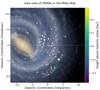 |
Fig. 1. Gaia EDR3 view of the 44 NS-HMXBs with good Gaia astrometry. Distance error bars correspond to 68% confidence intervals for the posterior of the reweighted parallax errors, obtained following Bailer-Jones et al. (2021) and Lindegren et al. (2021). The colour scheme of the error bars gives the distance to the Galactic plane. |
In order to compute galactocentric velocities from heliocentric equatorial coordinates, we use the GALACTOCENTRIC module from ASTROPY.COORDINATES. For this we assumed the position of the Galactic Centre in ICRS coordinates given by Reid & Brunthaler (2004,  ,
,  ), and the height of the Sun above the mid-Galactic plane of 27 pc (Chen et al. 2001), with a null roll angle. Furthermore, following Kawata et al. (2019), we considered the solar distance to the Galactic centre to be R⊙ = 8.2 kpc, with a Galactic rotation speed at the local standard of rest of vLSR = 236.0 km s−1, and a solar peculiar velocity of v⊙ = (8.0, 12.4, 7.7) km s−1 in Galactic coordinates. Once we obtain the galactocentric position and velocity of each source, to obtain their peculiar velocities vpec we subtracted the corresponding Galactic co-rotation velocity at each galactocentric position using the corresponding MWPOTENTIAL2014 solution from Bovy (2015).
For this purpose, during the MCMC calculations to infer the distance to the Gaia sources, we converted the proper motions to Galactic coordinates and, combining these values with the distance estimation, we obtained both the latitudinal and longitudinal peculiar velocities, which, added to the tangential peculiar velocity  , makes up the full peculiar velocity vector. For sources that have a systemic radial velocity (RV) measurement, we can directly estimate the full peculiar velocity vpec posterior. When no RV estimation was available (27 out of 44 sources), we filled in the peculiar velocity by assuming a random inclination for vpec, based on the estimated
  on the plane of the sky, and adopted a uniform prior in the 0−500 km s−1 range for the full peculiar velocity. In Table 2 we present mean values and 68% uncertainties for each of these posterior probability distributions for each source. Figure 2 illustrates the relation between companion masses and the inferred peculiar velocity for each HMXB that have a companion mass indicated in Table 1.
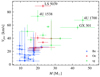 |
Fig. 2. Inferred peculiar velocities vs companion masses in the selected HMXBs. The uncertainty in mass come either from the literature (see Table 1) or from the 20% systematic described in Sect. 4; the uncertainty in peculiar velocity is the 68% confidence interval from the posteriors inferred in Sect. 3. |
We note that for the kick determination in the following section, we added an extra source of error to our inferences of peculiar velocities similar to a least count error. The peculiar velocity posteriors are broadened by a Gaussian with σ = 15 km s−1. This is to account for the fact that when we infer vpec ≤ 15 km s−1, the statistical error returned by our method becomes much lower than the typical velocity dispersion of the massive binary population. This dispersion was estimated for the population of young stars (0−150 Myr) in the thin disk of the Galaxy by Robin et al. (2003) to be between 10−20 km s−1, which should be applicable to our sample of HMXBs which are intrinsically young objects. Hence our choice to apply a broadening of 15 km s−1 for the peculiar velocities in the following calculations.
4. NS kick inference
Peculiar velocities carry indirect information about the natal kick incurred by the binary system. In this section we construct a MCMC algorithm to invert the orbital equations for an asymmetric SN explosion following the classical works from Brandt & Podsiadlowski (1995) and Kalogera (1996), to infer both the natal kick (w, whose magnitude we hereafter denote w) experienced by the NSs in HMXBs, as well as the pre-supernova masses (Mpre-SN) of the NS progenitors.
This method requires the orbital period of the NS HMXBs to be one of the inputs. From the 44 systems listed in Table 1, 35 have an orbital period estimation. In the following, we work only with these 35 source. Moreover, among these sources there are two systems for which we were not able to recover a companion mass using the means described in Sect. 2.4. The companion’s spectral type is not constrained enough to assign a mass using the spectral type tables. During the MCMC simulations, we chose to fill the missing values by a uniform random draw in an interval consistent with the spectral type of the companion: between 10−18 M⊙ for RX J2030.5+4751 (Be companion), and 10−53 M⊙ for XTE J1855−026 (supergiant companion). The mass ranges are based on the minimum and maximum companion masses we retrieved for Be and sg HMXBs. In all of the other 22 cases where no companion mass uncertainty was available, we used a 20% systematic error during the MCMC calculations, which we included through the likelihood. This value was chosen to reflect the relative error distribution on the companion mass in Table 1, which averages at 17 ± 9%.
In our treatment we assume that the orbit of each binary system is circular prior to SN core collapse. Most binaries born with a relatively short orbital period (up to two thousand days, depending on masses and metallicities; see e.g. Schneider et al. 2015) experience mass transfer through Roche-lobe overflow (RLO) or even a common-envelope (CE) phase. With the help of tidal forces (Dosopoulou & Kalogera 2016) the timescale for circularisation in such events should be shorter than the main sequence lifetime (Portegies Zwart & Verbunt 1996), so that just before the SN explosion the binary is likely to have already been circularised. A binary that does not circularise its orbit because of its initial large separation is instead more likely to be disrupted by the SN event (Kalogera 1996). It is therefore unlikely that systems in our NS HMXB list had significant eccentricity before the SN, even though a binary can start its evolution in a non-circular orbit.
In the absence of an asymmetry in the supernova explosion (w = 0), and considering no eccentricity prior to SN explosion, binary systems survive if less than half of the total system mass is lost during the SN (Blaauw 1961). In such a case, the post-SN eccentricity is directly proportional to the systemic velocity, vsys = epost-SNvorb (Kalogera 1996). Thus, it becomes evident that, under these assumptions, binary systems showing high systemic velocities and low eccentricities, as well as those systems with low systemic velocities and high eccentricities are hardly explained without invoking an asymmetric SN kick at birth (w ≫ 0).
The direction of the asymmetric kick could be affected by the orbital or rotational properties of the collapsing core. No clear connection between them was found or modelled in Kalogera (1996). However, Ng & Romani (2007) found that isolated pulsars may be preferentially kicked along their rotation axis if they are born with short (Pspin < 20 ms) or long (Pspin > 100 ms) spin periods. Intermediate spin pulsars would on the contrary suffer from kicks at almost perpendicular directions from their rotation axis.
Since we are dealing with binary systems, and since we do not have sufficient information on the spin axis and period of the NSs we are studying, we preferred to remain agnostic in the modelling of the kick. We thus assumed that the direction of the asymmetric kick is random; in other words that it is uniformly distributed in the sphere defined by the polar (θ) and azimutal (ϕ) angles with respect to the orbital velocity. In this scheme we ignored any possible interaction between the expanding supernova shell and its binary companion.
The equations from Kalogera (1996) relate the pre-SN system (M1, i, M2, i, Pi, ei) with those of the post-SN (M1, f, M2, f, Pf, ef, cos(i), vsys), after an arbitrary natal kick is applied (w, given by its magnitude w, and polar angles θ and ϕ), and the system loses a certain amount of mass ΔM = M1, f − M1, i. We note that ‘pre-SN’ denotes the stage right before the SN event, hence the pre-SN parameters take into account the potential mass transfer episodes preceding the SN event. In this work, we assumed that the companion mass is not affected by the SN explosion (M2, i = M2, f = M2). This is backed by Liu et al. (2015) in which the effect of the SN onto a companion star is shown to get smaller as the companion mass increases (simulations were performed using a 0.9 then a 3.5 M⊙ companion). Extrapolating to companions > 8 M⊙ would make the SN have an insignificant impact on the surviving companion stars in our sample. We also assumed that the binary system circularised before the SN explosion (ei = 0), as explained earlier, and that the NS mass was fixed to the canonical NS mass M1, f = 1.4 M⊙. The latter choice is backed by the observed NS mass distribution presented in Kiziltan et al. (2013) for double NS systems and NS-white dwarf binaries, which average respectively at 1.33 ± 0.1 M⊙ and 1.55 ± 0.25 M⊙. We thus used the intermediate value of 1.4 M⊙ which happens to be the one commonly used to assign a mass to a NS when no other information is available.
This leaves us with ten ‘free’ parameters, namely M1, i, M2, Pi, Pf, ef, cos(i), vsys, w, θ, and ϕ. On the one hand, part of these parameters can be directly compared to observed data: the companion mass (M2), the orbital period and eccentricity (Pf, ef), and the systemic velocity (vsys) inferred from the proper motion and radial velocity, when available. On the other hand, the pre-SN mass (M1, i = Mpre − SN), the pre-SN period (Pi), the inclination angle (cos(i)), and the natal kick (w) remain unknown, but can be inferred from the equations in a Bayesian scheme. We then constructed a likelihood comparing M2, Pf, ef, and vsys with the observables, and inferred the posterior-probability distributions of M1, i, Pi, cos(i), w, θ, and ϕ, assuming certain priors: isotropicity (by sampling θ and ϕ from a sphere), uniform natal kick in the 0 − 500 km s−1 range, and broad uniform priors on the pre-SN mass (M1, i uniform in 1.4 − 25 M⊙) and the pre-SN orbital period (Pi uniform in 1 − 103 d). We chose these simple priors in such a way to introduce the least amount of assumptions, trying to bias the results as little as possible.
We assumed that the likelihoods on period, eccentricity, and companion mass follow normal distributions. The width of the distributions are tied to the uncertainty of these parameters. For the companion masses we used the documented uncertainties in Table 1 when available; otherwise, we set it to 20% of the companion mass. The statistical errors on orbital period and eccentricity are very small; we chose to apply a 20% systematic as the width of the Gaussian likelihood. We note that for almost-circularised systems (e < 0.2) the likelihood for eccentricity is uniform in 0−0.25 instead of Gaussian. Choosing to apply large systematics to very constrained parameters is motivated by the potential evolution of those parameters during the post-SN epoch, even more so that we are dealing with accreting systems in which the masses and the orbits are affected by the mass and angular momentum transfer. This is backed by the observations of orbital period evolution in HMXBs that can go from a relative change of Ṗorb/Porb = 10−7 yr−1 (Levine et al. 1993, 2000; Safi Harb et al. 1996) up to 10−5 yr−1 (Kelley 1986). On an expected timescale since SN in HMXBs of a few 105 to 106 yr, this warrants the consideration of a difference between the orbital parameters in the current and post-SN epochs. The value we chose (20%) is empiric and could be addressed in the scope of more accurate binary evolution simulations.
Using the emcee sampler, we ran 200 walkers for 50 × 103 steps each. We burned in the first 20 × 103 steps of each individual chain, and combined and thinned them into a unique MCMC chain by randomly choosing 105 samples, which we used to obtain median and 68% credible intervals reported in Table 3. In Figs. 3 and 4 we present the posterior probability distributions of the kick magnitude (w) and pre-SN mass (MpreSN) of each HMXBs considered in this work. We use three different colours to separate the three different types of HMXBs according to the spectral type of the stellar companion (Be, Oe, sg).
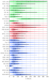 |
Fig. 3. Mirrored density plots of kick posteriors for individual binaries. The sg, Oe, and Be systems are shown in green, red, and blue, respectively. Posteriors are normalised to their maximum values. Source identifiers are cut for simplicity. |
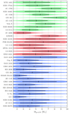 |
Fig. 4. Mirrored density plots of pre-SN mass posteriors. The sg, Oe, and Be systems are shown in green, red, and blue, respectively. Posteriors are normalised to their maximum values. Source identifiers are cut for simplicity. |
Inferred pre-SN properties and NS-kick strength for the 35 sources with determined orbital period and good astrometry.
Figure 3 shows the importance of having a complete set of observables to make a reliable inference of kick velocity. For instance, IGR J08408−4503 and XTE J1855−026 are two noteworthy sgHMXBs that we infer to have high kicks (> 200 km s−1). However, the latter is quite poorly constrained since we only have the proper motion, parallax, and orbital period to infer the kick. The extra companion mass, radial systemic velocity, and eccentricity make a much stronger case for the NS in IGR J08408−4503 to have experienced a very high natal kick.
5. Discussion
5.1. Peculiar velocities
In Fig. 2 we present the relation between the mass of the companion star and the inferred peculiar velocity. Taken as a whole, the sample shows a slight positive correlation between companion mass and peculiar velocity. The HMXBs containing Be donor stars have the lowest masses and lowest peculiar velocities in the sample, while the slightly more massive HMXBs hosting Oe donors reach the highest peculiar velocities. The sg HMXBs have a systematically high peculiar velocity, with little to no dependence on mass. Based on the obtained MpreSN distributions for each HMXB type (see Fig. 4 and Table 3) and under the assumption that the newly formed compact object is a NS, there is a wide range of ejecta masses associated with each HMXB type. BeHMXBs are associated with lower MpreSN compared to Oe and sgHMXBs.
A study on BeHMXBs and sgHMXBs (van den Heuvel et al. 2000) using Hipparcos data already anticipated a dichotomy between the two populations concerning their peculiar velocities. The authors provided two reasons, the first being linked to the higher fractional helium core mass of sgHMXB progenitors compared to BeHMXBs. The authors show that the higher primary mass in sgHMXBs progenitors leads to a higher helium core mass; in turn, the initial mass transfer from the primary to the companion leads to a smaller increase in orbital period compared to BeHMXB progenitors. This means that sgHMXBs tend to have tighter pre-SN orbits and higher orbital velocities compared to BeHMXBs. The second reason comes from the lower mass ejection in Be systems compared to supergiants during the SN event. Figure 2 shows this dichotomy between lower mass and supergiant systems, although we determined that the number of sources is too low to define a clear region in the mass-velocity plane. Roughly, the Be systems do not go beyond 40 km s−1 while only two out of nine supergiants are found below that limit.
The highest peculiar velocity we inferred is attributed to the OeHMXB LS 5039 (89 km s−1), and it is rather well-constrained thanks to the accuracy of the distance and radial velocity measurements for this source. It is noteworthy since all seven of the other OeHMXBs are inferred to have peculiar velocities between 20 and 40 km s−1. However, it is difficult to tell if the very high peculiar velocity of LS 5039 compared to the other OeHMXBs is an outlier or actually probes a specific mechanism that leads some systems to reach high peculiar velocities. One way to verify this would be to combine observations such as the ones used here with a detailed binary evolution study of the population of HMXBs with NS, which can set better constraints on the natal kicks for this population.
5.2. Kick velocity and populations
In this section we characterise the observed kick distributions of the three HMXB types (Be, Oe, and sg) by using a bootstrapping method. With each iteration we randomly pick one kick velocity according to each individual posterior inferred in Sect. 4. One iteration thus results in a collection of N kick measurements for a population of N sources. For each type of binary, we perform 103 iterations to build a set of possible kick posteriors.
We fitted the probability density function (PDF) of each iteration with a gamma distribution (see Eq. (1)), which we chose to parametrise with its mean μ and its skewness s. The best-fitting parameters were found by minimising a χ2 function with a Levenberg-Marquardt algorithm using SCIPY (Jones et al. 2001):
In this way, for each type of HMXB we obtained a distribution of μ and s that best represent their kick velocities. We extracted the median and the 68% confidence interval of these two parameters using the same percentiles described in Sect. 3. The bootstraps over each kick probability distributions are plotted against a gamma function with the above-mentioned median parameters (see Fig. 5), in the form of cumulative distributions (CDFs). For completeness, we applied the same method to the whole set of 35 HMXBs (ALL).
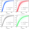 |
Fig. 5. Cumulative distributions of kicks obtained with the bootstrapping over each population (transparent) against the median results of the fit by a gamma function (opaque lines, 1σ errors are dotted). |
To quantify the goodness of fit over each population, we performed KS-tests of the median gamma distributions against each iteration of the bootstrap. The resulting p-value distributions all peak over 0.9, and less than 10% of the tests score lower than p = 0.1, indicating that the median gamma distributions accurately represent the data. We note that we first performed this bootstrapping method using Maxwellian distributions instead of gamma, and we found that the fits are poor across all HMXB types. This attempt at reproducing the NS HMXB kicks with Maxwellians is presented in Appendix A.
We note a difference in the mean velocity of the Be population versus the supergiant (μBe = 91 ± 16 km s−1 and  km s−1), while the Oe lie between these values at
  km s−1, indistinguishable from the other two. This is reflected in the two-sample KS-tests we performed between the three HMXB types, in which p-values for Be-Oe and Oe-sg both peak above 0.9, while the p-values of Be-sg are both flatter between 0.3−1 and extend further below 0.1. Possible dichotomic kick distributions according to different binary evolution channels for HMXBs have been explored in Brandt & Podsiadlowski (1995), notably regarding the stability of mass transfer events prior to the first SN explosion. Our results tend to agree with the presence of a dichotomy, although we believe that a bigger sample of binaries treated with our method could help to better constrain it.
The distributions of NS kicks in our list of HMXBs have an extra contribution at low velocities that can be explained in two ways. First, we cannot account for unbound systems that suffered very high kicks and second, there is a possibility (although still under debate) that the binaries we study have interacted before the SN event, leading to a stripped progenitor and resulting in overall smaller kicks (Willcox et al. 2021).
Lastly, this extra contribution at low velocities could challenge our hypothesis of the presence of a NS in each of our HMXBs. As stated in Sect. 2.5, 28 of them are confirmed to have a pulse period. We have inferred NS kick magnitudes for 24 of them. If the low-velocity contribution arises from the presence of a BH instead of a NS in some of the remaining 11 HMXBs in Table 3, we can roughly estimate how many BH HMXBs there are by refitting the gamma distributions to this subsample of 11 sources. After performing this, we obtained seemingly identical results to those presented in Fig. 5, albeit with higher error bars on the fitted parameters in accordance with the lower sample size.
We also checked the consistency between the inferred kicks and the orbital period and eccentricity of the binaries, as we would expect BH HMXBs to have low kicks, low orbital periods, and low eccentricities. None of the binaries in our sample meet the three criteria. The only binary with a low kick (< 50 km s−1) and low eccentricity (e ∼ 0.1) is X Per, which is confirmed to bear a NS since the discovery of its pulse period (Staubert et al. 2019). The three binaries with low orbital periods and eccentricities (Porb < 10 d, e < 0.1) are Vela X-1, 4U 1538−522, and 4U 1700−377; they all have higher kicks and are also confirmed to have a pulse period (Staubert et al. 2019; van den Eijnden et al. 2021), thus harbouring a NS. Based on these arguments and our search for catalogued BH HMXBs in Sect. 2.5, we conclude that it is unlikely that our sample of HMXBs contains any significant number of BH HMXBs that may have impacted the kick magnitude distributions.
5.3. Impact of missing systemic radial velocity
Our full sample of NS HMXBs (17 Be, 8 Oe, 10 sg) is quite heterogeneous concerning the available measurements on systemic radial velocity (4 Be, 5 Oe, 8 sg), which is necessary to properly infer the full peculiar velocity and NS kick vectors. We discuss in Sect. 3 the method we used to palliate this issue; here we present an overview of the impact of such method.
We only focused on systems with a measure of the systemic radial velocity, and performed the same analysis as described in Sect. 5.2. Again, the gamma distribution represents best the distributions of kick posteriors for individual types of NS HMXBs (Be, Oe, sg) and for the full sample (ALL). The fitted parameters of the gamma distributions are compatible within 1σ of those we derive in Sect. 5.2 on the entire set of binaries. We fit mean velocities of μBe = 79 km s−1,
  km s−1, and
  km s−1. The mean kick velocity of all the HMXB types combined is fitted at
  km s−1, which is seemingly the same as the one derived in Sect. 5.2, although with larger uncertainties (by a factor of ∼1.4). At N = 35 for the full sample and N = 17 for binaries with systemic radial velocity only, the change in uncertainty is exactly equal to the value we expect if we consider the change in sample size (
 ). At this stage, considering only NS HMXBs with an accurate measure of the systemic radial velocity does not allow for a finer determination of their kick as a population.
As for why the number of measurements on systemic radial velocity are so heterogeneous, and in particular highly in favour of sgHMXBs, a first explanation could be simply linked to the low sample numbers and statistical fluctuation. A second explanation could come from a selection effect: supergiant companions tend to be brighter, and are thus easier to get spectral time series on. However, according to the distribution of G magnitudes in our list of HMXBs, the two sgHMXBs that do not have any RV measurement fall within the magnitude limit in which we start to see other HMXBs with a determined RV (about G = 13.5). So their brightness should not be an obstacle for RV determination. The rest of the sgHMXB with determined RV are not brighter on average than the Be and Oe with determined RV. Looking at the dates of publications of the studies we found RVs in, most happened during the time the INTEGRAL satellite was operational (2003 to today). Since this mission discovered many sgHMXBs, it may also have caused an incentive to focus more on observing those systems in the optical–nIR, hence the high fraction of sgHMXBs with an RV determination (especially compared to BeHMXBs); however, this is purely speculative.
5.4. Impact of companion mass sampling
As stated in Sect. 4, we do not have a mass determination for the BeHMXB RX J2030.5+4751 and for the sgHMXB XTE J1855−026; to infer their natal kick magnitude, we adopted a uniform sampling of the companion mass during the MCMC calculations according to the range of masses found in their respective HMXB types (Be and sg). This method produces two main effects. First, the effective companion mass uncertainty is greater compared to the rest of our sources. Second, this arbitrarily sets the average companion mass at the centre of the mass range, which may heavily bias our kick magnitude estimation in the case the true companion mass lies at either of the range boundaries. Compared to all the other HMXBs kick estimation, the first effect appears negligible as the kick magnitude error bars are not significantly larger for the two sources (see Table 3). Mass uncertainty is thus not a predominant source of statistical error in the final inference in this case. As for the potential presence of a systematic error in the companion mass, this could heavily change the magnitude of the kick in either direction if the true mass is different from the mean of the mass range. While this effect should still be marginal for the BeHMXB since the mass range is rather small, the mass range for the sgHMXB is much greater. For XTE J1855−026, if we refer to the kick magnitude posteriors in Fig. 3 and compare the other sgHMXB kick posteriors, we find that it is one of the two sgHMXBs with very high kicks (> 200 km s−1). It is more likely that we overestimated the NS kick magnitude for this particular source, and that the true mass is in fact on the lower side of the 10−53 M⊙ range.
5.5. Neutron star velocities from disrupted systems
The work of Tauris & Takens (1998) provides analytical equations for the resulting space velocity of a neutron star that is kicked out of a binary after undergoing a supernova event. We implemented those equations in our MCMC calculations, in the cases where the kick disrupts the HMXBs (i.e. when the post-SN eccentricity is ≥1 or negative). For each of our HMXBs we obtained the distribution of NS velocity at infinity in the case of disruption (which can vary from 5 to 56%, of the outcomes depending on the system; see the runaway fraction in Table 3). As expected, we find that the average NS velocity in each case is proportional to the kick magnitude we derive.
We compared the full NS velocity distribution across our HMXB sample to the observed velocity distributions of isolated radio pulsars. Hobbs et al. (2005) showed that the 3D velocity of 233 known pulsars can be reproduced by a Maxwellian distribution at σ = 265 km s−1. More recently, Igoshev (2020) reported on distributions fitted either by a single Maxwellian of width σ = 229 km s−1, or a bimodal Maxwellian with σ1 = 146 km s−1 (∼60%) and σ2 = 317 km s−1 (∼40%). Our data cannot be reproduced by a bimodal Maxwellian; a unimodal Maxwellian fits rather poorly, with a width σ ∼ 110 km s−1. We note that a gamma distribution fits slightly better than a Maxwellian, and provides a mean velocity of 240 km s−1 with a skewness of 1.2, but the fit is still not satisfactory.
Since the systems we study here have by definition survived the supernova event, it is not surprising that their pre-SN orbital configuration tends not to produce high-velocity isolated NSs, hence the isolated NS velocities we derive are lower on average than the observed population of isolated radio pulsars. Although binary evolution can produce high-velocity NSs, our data suggests that less than 3% of the outcomes results in NSs with velocities greater than 500 km s−1, and these come from systems with pre-SN orbital periods of at least a few hundred days, if not upward of 1000 days.
6. Conclusion
Aiming to put constraints on natal kicks experienced in observed NS HMXBs using geometric and kinematic data, we gathered a sample of HMXBs from the literature that were observed by the Gaia satellite. We derived their peculiar velocities by using their position (3D) and proper motion (2D) from Gaia data, and by retrieving their systemic radial velocity (1D) from literature. This 6D data allowed us to infer posterior distributions of NS natal kicks by running MCMC simulations of the HMXB orbits when undergoing their first SN event. In our sample of binaries, 44 had sufficient accuracy in their astrometry to derive peculiar velocity, and 35 had additional orbital parameters needed to infer natal kicks and pre-SN primary mass posteriors. Differences in kick velocities between types of HMXBs were anticipated (Brandt & Podsiadlowski 1995), and our results hint at a dichotomy between Be and sg HMXBs. Be systems tend to have low NS kick compared to systems hosting a supergiant companion. In agreement with van den Heuvel et al. (2000), we find that the peculiar velocity of sgHMXBs is systematically high, even for supergiant companions of mass comparable to Be systems (10−18 M⊙).
The kick distributions we infer cannot be reproduced by Maxwellian statistics. We find that the inferred distributions are better represented by gamma functions, which incorporate an extra degree of freedom, and help to fit for a excess at low kick velocities (≲50 km s−1), which coexist with a broad distribution with significant support at high kick velocities (> 200 km s−1, see Appendix A). This low-velocity excess could be related to the fact that we study the subsample of NSs that are effectively observed as members of HMXBs, compared to the full NS population. Lower kick velocities are favoured in these systems, firstly because high kick velocities should lead to a higher fraction of unbound systems and secondly because most NSs present in HMXBs might evolve from stripped-envelope progenitors from mass transfer to their companion stars. Moreover, our inference is based on isotropicity in the kicks, a hypothesis that has been challenged for isolated pulsars in more recent studies (e.g. Ng & Romani 2007; Noutsos et al. 2013), thus possibly pointing to more complex underlying kick distributions.
Our sample of HMXBs might suffer from unaccounted selection effects coming from the cut we performed in the quality of the Gaia parallax; however, we have HMXBs lying at distances greater than 8 kpc, so we are likely probing a representative sample of the general population of HMXBs in the Milky Way. In terms of binary evolution, there are two limiting factors in this study. First and foremost, each system has a peculiar velocity imprinted at birth that we did not measure individually, but instead chose to model as a velocity dispersion following Robin et al. (2017). Knowing the individual birth conditions of each binary could inform us on that, but would also require studies dedicated to finding how HMXBs are born (e.g. isolated or in clusters). Secondly, the orbital parameters of HMXBs might change from post-SN to what is observed today, due to mass and angular momentum exchange, wind mass loss from the secondary, proportionally to the time spent since the SN event. A better modelling of this could be done on individual HMXBs using binary evolution simulations, which are usually performed on this type of sources in the scope of forming double compact merger candidates (see e.g. Marchant et al. 2016).
With the upcoming release of gravitational wave (GW) source catalogues from the LIGO/Virgo collaborations (e.g. GWTC-2, Abbott et al. 2021b), we will soon have access to a very wide range of observables on binaries, from the high-energy radiation coming from the vicinity of compact objects during accreting phases to the gravitational waves emitted during the last moments of a compact binary. When combined, they will span most of the evolutionary stages of binaries. More precisely, GW observations will bring information on the orbital parameters of compact binaries, which in turn will help to better constrain the key phases that affect those parameters, such as the kicks imparted by SN events and the common envelope episodes (see the review by Ivanova et al. 2013). For instance, García et al. (2021) study the impact of both kicks and common envelope on the recreation of the merger events GW 151226 and GW 170608 using hydrodynamical simulations of stellar evolution.
Lastly, we think that we should keep pushing to perform classical observations on HMXBs as we are still in great need of homogeneous data on these sources. Direct measurements done at evolutionary stages close to the SN event are especially valuable since they are less affected by binary evolution than they are at the endpoint of their life. Observables such as systemic radial velocities, companion masses, periods, and eccentricities are yet to be determined on well-known HMXBs in the Milky Way: photometry and spectroscopy in X-rays, optical, IR, and radio still have a lot to bring. Depicting the full picture of today’s X-ray binaries is necessary for us to have a more informed view of their evolution.
Acknowledgments
The authors were supported by the LabEx UnivEarthS, Interface project I10, “From evolution of binaries to merging of compact objects” and Interface project “Binary rEvolution”. The authors would like to thank Thierry Foglizzo, Jérôme Guillet and Thomas Tauris for fruitful discussions during the writing of this paper. This research has made use of the SIMBAD database, operated at CDS, Strasbourg, France. This work has made use of data from the European Space Agency (ESA) mission Gaia (https://www.cosmos.esa.int/Gaia), processed by the Gaia Data Processing and Analysis Consortium (DPAC, https://www.cosmos.esa.int/web/Gaia/dpac/consortium). Funding for the DPAC has been provided by national institutions, in particular the institutions participating in the Gaia Multilateral Agreement. Software. IPYTHON/JUPYTER (Perez & Granger 2007), MATPLOTLIB (Hunter 2007), NUMPY (van der Walt et al. 2011), SCIPY (Jones et al. 2001) and PYTHON from python.org. MCMC samples were obtained with the EMCEE package (Foreman-Mackey et al. 2013). This research made use of ASTROPY, a community-developed core PYTHON package for astronomy (Astropy Collaboration 2013, 2018).
References
- Abbott, R., Abbott, T. D., Abraham, S., et al. 2021a, ApJ, 913, L7 [NASA ADS] [CrossRef] [Google Scholar]
- Abbott, R., Abbott, T. D., Abraham, S., et al. 2021b, Phys. Rev. X, 11, 021053 [Google Scholar]
- Abubekerov, M. K., Antokhina, É. A., & Cherepashchuk, A. M. 2004, Astron. Rep., 48, 89 [NASA ADS] [CrossRef] [Google Scholar]
- An, H., Bellm, E., Bhalerao, V., et al. 2015, ApJ, 806, 166 [NASA ADS] [CrossRef] [Google Scholar]
- Aragona, C., McSwain, M. V., Grundstrom, E. D., et al. 2009, ApJ, 698, 514 [Google Scholar]
- Aragona, C., McSwain, M. V., & De Becker, M. 2010, ApJ, 724, 306 [Google Scholar]
- Astropy Collaboration (Robitaille, T. P., et al.) 2013, A&A, 558, A33 [NASA ADS] [CrossRef] [EDP Sciences] [Google Scholar]
- Astropy Collaboration (Price-Whelan, A. M., et al.) 2018, AJ, 156, 123 [Google Scholar]
- Atri, P., Miller-Jones, J. C. A., Bahramian, A., et al. 2019, MNRAS, 489, 3116 [NASA ADS] [CrossRef] [Google Scholar]
- Baibhav, V., Berti, E., Gerosa, D., et al. 2019, Phys. Rev. D, 100, 064060 [NASA ADS] [CrossRef] [Google Scholar]
- Bailer-Jones, C. A. L., Rybizki, J., Fouesneau, M., Demleitner, M., & Andrae, R. 2021, AJ, 161, 147 [Google Scholar]
- Baykal, A., Inam, S. Ç., Stark, M. J., et al. 2007, MNRAS, 374, 1108 [NASA ADS] [CrossRef] [Google Scholar]
- Bikmaev, I. F., Nikolaeva, E. A., Shimansky, V. V., et al. 2017, Astron. Lett., 43, 664 [NASA ADS] [CrossRef] [Google Scholar]
- Bird, A. J., Bazzano, A., Malizia, A., et al. 2016, ApJS, 223, 15 [Google Scholar]
- Blaauw, A. 1961, Bull. Astron. Inst. Neth., 15, 265 [NASA ADS] [Google Scholar]
- Blay, P., Negueruela, I., Reig, P., et al. 2006, A&A, 446, 1095 [NASA ADS] [CrossRef] [EDP Sciences] [Google Scholar]
- Bonnet-Bidaud, J. M., & Mouchet, M. 1998, A&A, 332, L9 [NASA ADS] [Google Scholar]
- Bovy, J. 2015, ApJS, 216, 29 [NASA ADS] [CrossRef] [Google Scholar]
- Brandt, N., & Podsiadlowski, P. 1995, MNRAS, 274, 461 [NASA ADS] [CrossRef] [Google Scholar]
- Brown, A. G. A., Vallenari, A., Prusti, T., et al. 2021, A&A, 649, A1 [NASA ADS] [CrossRef] [EDP Sciences] [Google Scholar]
- Casares, J., Ribas, I., Paredes, J. M., Martí, J., & Allende Prieto, C. 2005a, MNRAS, 360, 1105 [NASA ADS] [CrossRef] [Google Scholar]
- Casares, J., Ribó, M., Ribas, I., et al. 2005b, MNRAS, 364, 899 [Google Scholar]
- Casares, J., Corral-Santana, J. M., Herrero, A., et al. 2011, Ap&SS, 21, 599 [Google Scholar]
- Casares, J., Negueruela, I., Ribó, M., et al. 2014, Nature, 505, 378 [Google Scholar]
- Chaty, S. 2013, Adv. Space Res., 52, 2132 [NASA ADS] [CrossRef] [Google Scholar]
- Chen, B., Stoughton, C., Smith, J. A., et al. 2001, ApJ, 553, 184 [Google Scholar]
- Coe, M. J., Longmore, A., Payne, B. J., & Hanson, C. G. 1988, MNRAS, 232, 865 [NASA ADS] [CrossRef] [Google Scholar]
- Coe, M. J., Roche, P., Everall, C., et al. 1994, MNRAS, 270, L57 [NASA ADS] [Google Scholar]
- Coleiro, A., & Chaty, S. 2013, ApJ, 764, 185 [NASA ADS] [CrossRef] [Google Scholar]
- Coleiro, A., Chaty, S., Zurita Heras, J. A., Rahoui, F., & Tomsick, J. A. 2013, A&A, 560, A108 [NASA ADS] [CrossRef] [EDP Sciences] [Google Scholar]
- Corbet, R. H. D., & Krimm, H. A. 2010, ATel, 3079, 1 [NASA ADS] [Google Scholar]
- Corral-Santana, J. M., Casares, J., Muñoz-Darias, T., et al. 2016, A&A, 587, A61 [NASA ADS] [CrossRef] [EDP Sciences] [Google Scholar]
- Crampton, D., Hutchings, J. B., & Cowley, A. P. 1985, ApJ, 299, 839 [NASA ADS] [CrossRef] [Google Scholar]
- Delgado-Martí, H., Levine, A. M., Pfahl, E., & Rappaport, S. A. 2001, ApJ, 546, 455 [CrossRef] [Google Scholar]
- Densham, R. H., & Charles, P. A. 1982, MNRAS, 201, 171 [NASA ADS] [CrossRef] [Google Scholar]
- Dosopoulou, F., & Kalogera, V. 2016, ApJ, 825, 70 [NASA ADS] [CrossRef] [Google Scholar]
- Evans, P. A., Osborne, J. P., Beardmore, A. P., et al. 2014, ApJS, 210, 8 [Google Scholar]
- Evans, I. N., Allen, C., Anderson, C. S., et al. 2019, Am. Astron. Soc. Meet. Abstr., 233, 379.01 [NASA ADS] [Google Scholar]
- Falanga, M., Bozzo, E., Lutovinov, A., et al. 2015, A&A, 577, A130 [NASA ADS] [CrossRef] [EDP Sciences] [Google Scholar]
- Ferrigno, C., Farinelli, R., Bozzo, E., et al. 2013, A&A, 553, A103 [NASA ADS] [CrossRef] [EDP Sciences] [Google Scholar]
- Finger, M. H., Wilson, R. B., & Harmon, B. A. 1996, ApJ, 459, 288 [NASA ADS] [CrossRef] [Google Scholar]
- Foreman-Mackey, D., Hogg, D. W., Lang, D., & Goodman, J. 2013, PASP, 125, 306 [Google Scholar]
- Fortin, F., Chaty, S., Coleiro, A., Tomsick, J. A., & Nitschelm, C. H. R. 2018, A&A, 618, A150 [NASA ADS] [CrossRef] [EDP Sciences] [Google Scholar]
- Fryer, C. L., & Kusenko, A. 2006, ApJS, 163, 335 [NASA ADS] [CrossRef] [Google Scholar]
- Gaia Collaboration (Prusti, T., et al.) 2016, A&A, 595, A1 [NASA ADS] [CrossRef] [EDP Sciences] [Google Scholar]
- Gamen, R., Barbà, R. H., Walborn, N. R., et al. 2015, A&A, 583, L4 [NASA ADS] [CrossRef] [EDP Sciences] [Google Scholar]
- García, F., Simaz Bunzel, A., Chaty, S., Porter, E., & Chassande-Mottin, E. 2021, A&A, 649, A114 [NASA ADS] [CrossRef] [EDP Sciences] [Google Scholar]
- Gies, D. R., & Bolton, C. T. 1986, ApJS, 61, 419 [Google Scholar]
- Gregory, P. C. 2002, ApJ, 575, 427 [NASA ADS] [CrossRef] [Google Scholar]
- Grimm, H.-J., Gilfanov, M., & Sunyaev, R. 2002, A&A, 391, 923 [NASA ADS] [CrossRef] [EDP Sciences] [Google Scholar]
- Grundstrom, E. D., Boyajian, T. S., Finch, C., et al. 2007, ApJ, 660, 1398 [NASA ADS] [CrossRef] [Google Scholar]
- Grunhut, J. H., Bolton, C. T., & McSwain, M. V. 2014, A&A, 563, A1 [NASA ADS] [CrossRef] [EDP Sciences] [Google Scholar]
- Hansen, B. M. S., & Phinney, E. S. 1997, MNRAS, 291, 569 [NASA ADS] [Google Scholar]
- Hobbs, G., Lorimer, D. R., Lyne, A. G., & Kramer, M. 2005, MNRAS, 360, 974 [Google Scholar]
- Houk, N. 1978, Michigan Catalogue of Two-dimensional Spectral Types for the HD Stars (Ann Arbor: Dept. of Astronomy, University of Michigan) [Google Scholar]
- Hu, C.-P., Chou, Y., Ng, C. Y., Lin, L. C.-C., & Yen, D. C.-C. 2017, ApJ, 844, 16 [NASA ADS] [CrossRef] [Google Scholar]
- Hunter, J. D. 2007, Comput. Sci. Eng., 9, 90 [NASA ADS] [CrossRef] [Google Scholar]
- Hutchings, J. B. 1984, PASP, 96, 312 [NASA ADS] [CrossRef] [Google Scholar]
- Hutchings, J. B., Cowley, A. P., Crampton, D., & Williams, G. 1981, PASP, 93, 741 [NASA ADS] [CrossRef] [Google Scholar]
- Hutchings, J. B., Crampton, D., Cowley, D., Cowley, A. P., & Bord, D. J. 1982, PASP, 94, 541 [NASA ADS] [CrossRef] [Google Scholar]
- Hutchings, J. B., Crampton, D., Cowley, A. P., & Thompson, I. B. 1987, PASP, 99, 420 [NASA ADS] [CrossRef] [Google Scholar]
- Hynes, R. I., Clark, J. S., Barsukova, E. A., et al. 2002, A&A, 392, 991 [NASA ADS] [CrossRef] [EDP Sciences] [Google Scholar]
- Igoshev, A. P. 2020, MNRAS, 494, 3663 [NASA ADS] [CrossRef] [Google Scholar]
- in’t Zand, J. J. M., Halpern, J., Eracleous, M., et al. 2000, A&A, 361, 85 [Google Scholar]
- in’t Zand, J. J. M., Kuiper, L., den Hartog, P. R., Hermsen, W., & Corbet, R. H. D. 2007, A&A, 469, 1063 [CrossRef] [EDP Sciences] [Google Scholar]
- Islam, N., & Paul, B. 2016, MNRAS, 461, 816 [NASA ADS] [CrossRef] [Google Scholar]
- Ivanova, N., Justham, S., Chen, X., et al. 2013, A&ARv, 21, 59 [Google Scholar]
- Janka, H.-T. 2013, MNRAS, 434, 1355 [Google Scholar]
- Janot-Pacheco, E., Ilovaisky, S. A., & Chevalier, C. 1981, A&A, 99, 274 [NASA ADS] [Google Scholar]
- Jaschek, M., & Egret, D. 1982, in Be Stars, eds. M. Jaschek, & H. G. Groth, 98, 261 [Google Scholar]
- Johnston, S., Manchester, R. N., Lyne, A. G., Nicastro, L., & Spyromilio, J. 1994, MNRAS, 268, 430 [NASA ADS] [Google Scholar]
- Jones, E., Oliphant, T., Peterson, P., et al. 2001, SciPy: Open Source Scientific Tools for Python, http://www.scipy.org [Google Scholar]
- Kaaret, P., Piraino, S., Halpern, J., & Eracleous, M. 1999, ApJ, 523, 197 [NASA ADS] [CrossRef] [Google Scholar]
- Kaaret, P., Cusumano, G., & Sacco, B. 2000, ApJ, 542, L41 [NASA ADS] [CrossRef] [Google Scholar]
- Kabiraj, S., & Paul, B. 2020, MNRAS, 497, 1059 [NASA ADS] [CrossRef] [Google Scholar]
- Kalogera, V. 1996, ApJ, 471, 352 [Google Scholar]
- Kaper, L., van der Meer, A., & Najarro, F. 2006, A&A, 457, 595 [CrossRef] [EDP Sciences] [Google Scholar]
- Kaur, R., Paul, B., Kumar, B., & Sagar, R. 2008, MNRAS, 386, 2253 [NASA ADS] [CrossRef] [Google Scholar]
- Kawata, D., Bovy, J., Matsunaga, N., & Baba, J. 2019, MNRAS, 482, 40 [NASA ADS] [CrossRef] [Google Scholar]
- Kelley, R. L. 1986, NATO Advanced Study Institute (ASI) Series C, 167, 75 [NASA ADS] [Google Scholar]
- Kiziltan, B., Kottas, A., De Yoreo, M., & Thorsett, S. E. 2013, ApJ, 778, 66 [NASA ADS] [CrossRef] [Google Scholar]
- Koenigsberger, G., Canalizo, G., Arrieta, A., Richer, M. G., & Georgiev, L. 2003, Rev. Mex. Astron. Astrofis., 39, 17 [Google Scholar]
- Koenigsberger, G., Georgiev, L., Moreno, E., et al. 2006, A&A, 458, 513 [NASA ADS] [CrossRef] [EDP Sciences] [Google Scholar]
- Krtička, J., Kubát, J., & Krtičková, I. 2015, A&A, 579, A111 [NASA ADS] [CrossRef] [EDP Sciences] [Google Scholar]
- La Palombara, N., & Mereghetti, S. 2017, A&A, 602, A114 [NASA ADS] [CrossRef] [EDP Sciences] [Google Scholar]
- Lai, D., Chernoff, D. F., & Cordes, J. M. 2001, ApJ, 549, 1111 [NASA ADS] [CrossRef] [Google Scholar]
- Landi, R., Bassani, L., Bazzano, A., et al. 2017, MNRAS, 470, 1107 [CrossRef] [Google Scholar]
- Levine, A., Rappaport, S., Deeter, J. E., Boynton, P. E., & Nagase, F. 1993, ApJ, 410, 328 [NASA ADS] [CrossRef] [Google Scholar]
- Levine, A. M., Rappaport, S. A., & Zojcheski, G. 2000, ApJ, 541, 194 [NASA ADS] [CrossRef] [Google Scholar]
- Lindegren, L., Bastian, U., Biermann, M., et al. 2021, A&A, 649, A4 [EDP Sciences] [Google Scholar]
- Liu, Q. Z., van Paradijs, J., & van den Heuvel, E. P. J. 2006, A&A, 455, 1165 [NASA ADS] [CrossRef] [EDP Sciences] [Google Scholar]
- Liu, Z.-W., Tauris, T. M., Röpke, F. K., et al. 2015, A&A, 584, A11 [NASA ADS] [CrossRef] [EDP Sciences] [Google Scholar]
- Lopes de Oliveira, R., Motch, C., Haberl, F., Negueruela, I., & Janot-Pacheco, E. 2006, A&A, 454, 265 [NASA ADS] [CrossRef] [EDP Sciences] [Google Scholar]
- Lyne, A. G., & Lorimer, D. R. 1994, Nature, 369, 127 [NASA ADS] [CrossRef] [Google Scholar]
- Lyubimkov, L. S., Rostopchin, S. I., Roche, P., & Tarasov, A. E. 1997, MNRAS, 286, 549 [NASA ADS] [CrossRef] [Google Scholar]
- Marchant, P., Langer, N., Podsiadlowski, P., Tauris, T. M., & Moriya, T. J. 2016, A&A, 588, A50 [NASA ADS] [CrossRef] [EDP Sciences] [Google Scholar]
- Marrese, P. M., Marinoni, S., Fabrizio, M., & Altavilla, G. 2019, A&A, 621, A144 [NASA ADS] [CrossRef] [EDP Sciences] [Google Scholar]
- Martins, F., Schaerer, D., & Hillier, D. J. 2005, A&A, 436, 1049 [NASA ADS] [CrossRef] [EDP Sciences] [Google Scholar]
- Masetti, N., Mason, E., Morelli, L., et al. 2008, A&A, 482, 113 [NASA ADS] [CrossRef] [EDP Sciences] [Google Scholar]
- Masetti, N., Parisi, P., Palazzi, E., et al. 2009, A&A, 495, 121 [NASA ADS] [CrossRef] [EDP Sciences] [Google Scholar]
- Masetti, N., Parisi, P., Palazzi, E., et al. 2010, A&A, 519, A96 [NASA ADS] [CrossRef] [EDP Sciences] [Google Scholar]
- Masetti, N., Parisi, P., Palazzi, E., et al. 2013, A&A, 556, A120 [NASA ADS] [CrossRef] [EDP Sciences] [Google Scholar]
- McBride, V. A., Wilms, J., Kreykenbohm, I., et al. 2007, A&A, 470, 1065 [NASA ADS] [CrossRef] [EDP Sciences] [Google Scholar]
- Miller-Jones, J. C. A., Deller, A. T., Shannon, R. M., et al. 2018, MNRAS, 479, 4849 [Google Scholar]
- Mirabel, I. F., Mignani, R., Rodrigues, I., et al. 2002, A&A, 395, 595 [NASA ADS] [CrossRef] [EDP Sciences] [Google Scholar]
- Moritani, Y., Kawano, T., Chimasu, S., et al. 2018, PASJ, 70, 61 [NASA ADS] [Google Scholar]
- Negueruela, I., & Okazaki, A. T. 2001, A&A, 369, 108 [NASA ADS] [CrossRef] [EDP Sciences] [Google Scholar]
- Negueruela, I., Roche, P., Fabregat, J., & Coe, M. J. 1999, MNRAS, 307, 695 [NASA ADS] [CrossRef] [Google Scholar]
- Negueruela, I., Casares, J., Verrecchia, F., et al. 2008, ATel, 1876, 1 [Google Scholar]
- Negueruela, I., Ribó, M., Herrero, A., et al. 2011, ApJ, 732, L11 [Google Scholar]
- Nespoli, E., Fabregat, J., & Mennickent, R. E. 2008, A&A, 486, 911 [NASA ADS] [CrossRef] [EDP Sciences] [Google Scholar]
- Ng, C. Y., & Romani, R. W. 2007, ApJ, 660, 1357 [NASA ADS] [CrossRef] [Google Scholar]
- Nikolaeva, E. A., Bikmaev, I. F., Melnikov, S. S., et al. 2013, Bull. Crime. Astrophys. Obs., 109, 27 [CrossRef] [Google Scholar]
- Noutsos, A., Schnitzeler, D. H. F. M., Keane, E. F., Kramer, M., & Johnston, S. 2013, MNRAS, 430, 2281 [NASA ADS] [CrossRef] [Google Scholar]
- Okazaki, A. T., & Negueruela, I. 2001, A&A, 377, 161 [NASA ADS] [CrossRef] [EDP Sciences] [Google Scholar]
- Pacheco, E. J., Chevalier, C., & Ilovaisky, S. A. 1982, in Be Stars, eds. M. Jaschek, & H. G. Groth, 98, 151 [NASA ADS] [CrossRef] [Google Scholar]
- Parkes, G. E., Murdin, P. G., & Mason, K. O. 1978, MNRAS, 184, 73 [Google Scholar]
- Parkes, G. E., Murdin, P. G., & Mason, K. O. 1980, MNRAS, 190, 537 [Google Scholar]
- Pellizza, L. J., Chaty, S., & Negueruela, I. 2006, A&A, 455, 653 [NASA ADS] [CrossRef] [EDP Sciences] [Google Scholar]
- Perez, F., & Granger, B. E. 2007, Comput. Sci. Eng., 9, 21 [Google Scholar]
- Podsiadlowski, P., Langer, N., Poelarends, A. J. T., et al. 2004, ApJ, 612, 1044 [NASA ADS] [CrossRef] [Google Scholar]
- Podsiadlowski, P., Pfahl, E., & Rappaport, S. 2005, in Binary Radio Pulsars, eds. F. A. Rasio, & I. H. Stairs, ASP Conf. Ser., 328, 327 [NASA ADS] [Google Scholar]
- Polcaro, V. F., Rossi, C., Giovannelli, F., et al. 1990, A&A, 231, 354 [NASA ADS] [Google Scholar]
- Portegies Zwart, S. F., & Verbunt, F. 1996, A&A, 309, 179 [NASA ADS] [Google Scholar]
- Porter, J. M. 1996, MNRAS, 280, L31 [NASA ADS] [CrossRef] [Google Scholar]
- Pradhan, P., Maitra, C., Paul, B., & Paul, B. C. 2013, MNRAS, 436, 945 [NASA ADS] [CrossRef] [Google Scholar]
- Raichur, H., & Paul, B. 2010, MNRAS, 406, 2663 [NASA ADS] [CrossRef] [Google Scholar]
- Ray, P. S., & Chakrabarty, D. 2002, ApJ, 581, 1293 [NASA ADS] [CrossRef] [Google Scholar]
- Reid, M. J., & Brunthaler, A. 2004, ApJ, 616, 872 [Google Scholar]
- Reig, P., Negueruela, I., Fabregat, J., et al. 2004, A&A, 421, 673 [NASA ADS] [CrossRef] [EDP Sciences] [Google Scholar]
- Reig, P., Negueruela, I., Papamastorakis, G., Manousakis, A., & Kougentakis, T. 2005a, A&A, 440, 637 [NASA ADS] [CrossRef] [EDP Sciences] [Google Scholar]
- Reig, P., Negueruela, I., Fabregat, J., Chato, R., & Coe, M. J. 2005b, A&A, 440, 1079 [NASA ADS] [CrossRef] [EDP Sciences] [Google Scholar]
- Reig, P., Blay, P., & Blinov, D. 2017, A&A, 598, A16 [NASA ADS] [CrossRef] [EDP Sciences] [Google Scholar]
- Repetto, S., Igoshev, A. P., & Nelemans, G. 2017, MNRAS, 467, 298 [Google Scholar]
- Rivinius, T., Carciofi, A. C., & Martayan, C. 2013, A&ARv, 21, 69 [Google Scholar]
- Robin, A. C., Reylé, C., Derrière, S., & Picaud, S. 2003, A&A, 409, 523 [NASA ADS] [CrossRef] [EDP Sciences] [Google Scholar]
- Robin, A. C., Bienaymé, O., Fernández-Trincado, J. G., & Reylé, C. 2017, A&A, 605, A1 [NASA ADS] [CrossRef] [EDP Sciences] [Google Scholar]
- Rohatgi, A. 2021, Webplotdigitizer: Version 4.5, https://automeris.io/WebPlotDigitizer [Google Scholar]
- Romero-Gómez, M., Mateu, C., Aguilar, L., Figueras, F., & Castro-Ginard, A. 2019, A&A, 627, A150 [NASA ADS] [CrossRef] [EDP Sciences] [Google Scholar]
- Safi Harb, S., Ogelman, H., & Dennerl, K. 1996, ApJ, 456, L37 [NASA ADS] [Google Scholar]
- Sanjurjo-Ferrrín, G., Torrejón, J. M., Postnov, K., et al. 2017, A&A, 606, A145 [NASA ADS] [CrossRef] [EDP Sciences] [Google Scholar]
- Schneider, F. R. N., Izzard, R. G., Langer, N., & de Mink, S. E. 2015, ApJ, 805, 20 [Google Scholar]
- Schwope, A. D., Worpel, H., Webb, N. A., Koliopanos, F., & Guillot, S. 2020, A&A, 637, A35 [NASA ADS] [CrossRef] [EDP Sciences] [Google Scholar]
- Sidoli, L., & Paizis, A. 2018, MNRAS, 481, 2779 [NASA ADS] [CrossRef] [Google Scholar]
- Skrutskie, M. F., Cutri, R. M., Stiening, R., et al. 2006, AJ, 131, 1163 [NASA ADS] [CrossRef] [Google Scholar]
- Slettebak, A. 1982, ApJS, 50, 55 [NASA ADS] [CrossRef] [Google Scholar]
- Sota, A., Maíz Apellániz, J., Morrell, N. I., et al. 2014, ApJS, 211, 10 [Google Scholar]
- Staubert, R., Trümper, J., Kendziorra, E., et al. 2019, A&A, 622, A61 [NASA ADS] [CrossRef] [EDP Sciences] [Google Scholar]
- Stickland, D., Lloyd, C., & Radziun-Woodham, A. 1997, MNRAS, 286, L21 [NASA ADS] [CrossRef] [Google Scholar]
- Stoyanov, K. A., Zamanov, R. K., Latev, G. Y., Abedin, A. Y., & Tomov, N. A. 2014, Astron. Nachr., 335, 1060 [NASA ADS] [CrossRef] [Google Scholar]
- Strader, J., Chomiuk, L., Cheung, C. C., Salinas, R., & Peacock, M. 2015, ApJ, 813, L26 [NASA ADS] [CrossRef] [Google Scholar]
- Tauris, T. M., & Takens, R. J. 1998, A&A, 330, 1047 [NASA ADS] [Google Scholar]
- Tauris, T. M., Fender, R. P., van den Heuvel, E. P. J., Johnston, H. M., & Wu, K. 1999, MNRAS, 310, 1165 [NASA ADS] [CrossRef] [Google Scholar]
- Taylor, M. B. 2005, ASP Conf. Ser., 347, 29 [Google Scholar]
- Townsend, L. J., Coe, M. J., Corbet, R. H. D., & Hill, A. B. 2011, MNRAS, 416, 1556 [NASA ADS] [CrossRef] [Google Scholar]
- Uchida, N., Takahashi, H., Fukazawa, Y., & Makishima, K. 2021, PASJ, 73, 1389 [NASA ADS] [CrossRef] [Google Scholar]
- van den Eijnden, J., Degenaar, N., Russell, T. D., et al. 2021, MNRAS, 507, 3899 [NASA ADS] [CrossRef] [Google Scholar]
- van den Heuvel, E. P. J., Portegies Zwart, S. F., Bhattacharya, D., & Kaper, L. 2000, A&A, 364, 563 [NASA ADS] [Google Scholar]
- van der Walt, S., Colbert, S. C., & Varoquaux, G. 2011, Comput. Sci. Eng., 13, 22 [Google Scholar]
- Vieira, S. L. A., Corradi, W. J. B., Alencar, S. H. P., et al. 2003, AJ, 126, 2971 [Google Scholar]
- Waisberg, I. R., & Romani, R. W. 2015, ApJ, 805, 18 [NASA ADS] [CrossRef] [Google Scholar]
- Walter, R., Lutovinov, A. A., Bozzo, E., & Tsygankov, S. S. 2015, A&ARv, 23, 2 [Google Scholar]
- Wang, Z. X., & Gies, D. R. 1998, PASP, 110, 1310 [Google Scholar]
- Weng, S.-S., Qian, L., Wang, B.-J., et al. 2022, Nat. Astron., 6, 698 [NASA ADS] [CrossRef] [Google Scholar]
- Wenger, M., Ochsenbein, F., Egret, D., et al. 2000, A&AS, 143, 9 [NASA ADS] [CrossRef] [EDP Sciences] [Google Scholar]
- Willcox, R., Mandel, I., Thrane, E., et al. 2021, ApJ, 920, L37 [NASA ADS] [CrossRef] [Google Scholar]
- Wilson, C. A., Finger, M. H., Harmon, B. A., Chakrabarty, D., & Strohmayer, T. 1998, ApJ, 499, 820 [NASA ADS] [CrossRef] [Google Scholar]
- Zorec, J., Frémat, Y., & Cidale, L. 2005, A&A, 441, 235 [NASA ADS] [CrossRef] [EDP Sciences] [Google Scholar]
Appendix A: Fitting NS HMXB kick distribution with Maxwellian functions
In Section 5.2 we characterised the observed NS kick magnitudes in HMXBs using gamma statistics. Here we present the same results, only using Maxwellian statistics.
The initial motivation to use Maxwellian to reproduce a distribution of kick velocities comes from historical studies focused on isolated pulsars. For instance, Hansen & Phinney (1997) show that the natal kick derived on a set of 86 isolated pulsars could be reproduced by a Maxwellian that would imply a characteristic velocity of 250 to 300 km s−1. The authors also note they find no evidence of a low-velocity contribution. However, in our case, we deal with systems that survived through the SN event.
For the sake of comparison, we attempted to fit the probability density function (PDF) of observed NS HMXB kicks with Maxwellian statistics, which we parametrised by the Maxwellian scale (scale) and localisation (loc). For this we used the Python SCIPY.STATS package (Jones et al. 2001), which provides a Maxwellian PDF defined by Equation (A.1):

In the first attempt, we fix the loc parameter to 0, which produces a standardised Maxwell distribution. As shown in Figure A.1, while the high-velocity regime is somewhat correctly reproduced, it fails to take into account the low-velocity tail. This results in an overall very poor fit, as demonstrated by the distribution of p-values from individual KS-tests performed at each fit iteration (see Figure A.2).
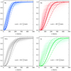 |
Fig. A.1. Cumulative distributions of kicks obtained with bootstrapping over each population (transparent) against the median results of the fit by a standardised Maxwell function (opaque lines, 1σ errors are dotted). |
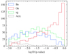 |
Fig. A.2. Distribution of the p-values associated with KS-tests performed after each iteration of Maxwellian fit (one free parameter). |
We then free the loc parameter to fit shifted Maxwell distributions instead. The results in Figure A.3 show an improvement over the single-parameter Maxwellian; this is also reflected in the distribution of the associated p-values (see Figure A.4). While the kick distributions are better reproduced than with a standard Maxwellian, the goodness of fit is at best unconvincing for OeHMXBs, rather poor for BeHMXBs and sgHMXBs, and extremely bad when considering the whole sample of HMXBs. Moreover, giving a physical interpretation to a negative offset (loc < 0 km s−1) in the Maxwellian distribution of kick velocities is challenging.
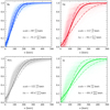 |
Fig. A.3. Cumulative distributions of kicks obtained with bootstrapping over each population (transparent) against the median results of the fit by a shifted Maxwell function (opaque lines, 1σ errors are dotted). |
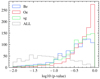 |
Fig. A.4. Distribution of the p-values associated with KS-tests performed after each iteration of Maxwellian fit (two free parameters). |
Thus, in the scope of this paper, we believe that the observed population of the Galactic NS HMXBs do not produce natal kick distributions that can be represented by Maxwellian statistics.
All Tables
Gaia information, inferred distances, and peculiar velocities of the 44 NS-HMXB sources with good astrometric data quality.
Inferred pre-SN properties and NS-kick strength for the 35 sources with determined orbital period and good astrometry.
All Figures
|
Fig. 1. Gaia EDR3 view of the 44 NS-HMXBs with good Gaia astrometry. Distance error bars correspond to 68% confidence intervals for the posterior of the reweighted parallax errors, obtained following Bailer-Jones et al. (2021) and Lindegren et al. (2021). The colour scheme of the error bars gives the distance to the Galactic plane. |
| In the text | |
|
Fig. 2. Inferred peculiar velocities vs companion masses in the selected HMXBs. The uncertainty in mass come either from the literature (see Table 1) or from the 20% systematic described in Sect. 4; the uncertainty in peculiar velocity is the 68% confidence interval from the posteriors inferred in Sect. 3. |
| In the text | |
|
Fig. 3. Mirrored density plots of kick posteriors for individual binaries. The sg, Oe, and Be systems are shown in green, red, and blue, respectively. Posteriors are normalised to their maximum values. Source identifiers are cut for simplicity. |
| In the text | |
|
Fig. 4. Mirrored density plots of pre-SN mass posteriors. The sg, Oe, and Be systems are shown in green, red, and blue, respectively. Posteriors are normalised to their maximum values. Source identifiers are cut for simplicity. |
| In the text | |
|
Fig. 5. Cumulative distributions of kicks obtained with the bootstrapping over each population (transparent) against the median results of the fit by a gamma function (opaque lines, 1σ errors are dotted). |
| In the text | |
|
Fig. A.1. Cumulative distributions of kicks obtained with bootstrapping over each population (transparent) against the median results of the fit by a standardised Maxwell function (opaque lines, 1σ errors are dotted). |
| In the text | |
|
Fig. A.2. Distribution of the p-values associated with KS-tests performed after each iteration of Maxwellian fit (one free parameter). |
| In the text | |
|
Fig. A.3. Cumulative distributions of kicks obtained with bootstrapping over each population (transparent) against the median results of the fit by a shifted Maxwell function (opaque lines, 1σ errors are dotted). |
| In the text | |
|
Fig. A.4. Distribution of the p-values associated with KS-tests performed after each iteration of Maxwellian fit (two free parameters). |
| In the text | |
Current usage metrics show cumulative count of Article Views (full-text article views including HTML views, PDF and ePub downloads, according to the available data) and Abstracts Views on Vision4Press platform.
Data correspond to usage on the plateform after 2015. The current usage metrics is available 48-96 hours after online publication and is updated daily on week days.
Initial download of the metrics may take a while.