| Issue |
A&A
Volume 664, August 2022
|
|
|---|---|---|
| Article Number | A77 | |
| Number of page(s) | 23 | |
| Section | Cosmology (including clusters of galaxies) | |
| DOI | https://doi.org/10.1051/0004-6361/202142479 | |
| Published online | 05 August 2022 | |
Pure-mode correlation functions for cosmic shear and application to KiDS-1000
1
Argelander-Institut für Astronomie, Universität Bonn, Auf dem Hügel 71, 53121 Bonn, Germany
e-mail: peter@astro.uni-bonn.de
2
Institute for Astronomy, University of Edinburgh, Royal Observatory, Blackford Hill, Edinburgh EH9 3HJ, UK
3
E. A. Milne Centre, University of Hull, Cottingham Road, Hull HU6 7RX, UK
4
Ruhr University Bochum, Faculty of Physics and Astronomy, Astronomical Institute (AIRUB), German Centre for Cosmological Lensing, 44780 Bochum, Germany
5
School of Mathematics, Statistics and Physics, Newcastle University, Herschel Building, NE1 7RU Newcastle-upon-Tyne, UK
6
Leiden Observatory, Leiden University, PO Box 9513 2300 RA Leiden, The Netherlands
7
Shanghai Astronomical Observatory (SHAO), Nandan Road 80, Shanghai 200030, PR China
8
University of Chinese Academy of Sciences, Beijing 100049, PR China
Received:
19
October
2021
Accepted:
8
March
2022
One probe for systematic effects in gravitational lensing surveys is the presence of so-called B modes in the cosmic shear two-point correlation functions, ξ±(ϑ), since lensing is expected to produce only E-mode shear. Furthermore, there exist ambiguous modes that cannot uniquely be assigned to either E- or B-mode shear. In this paper we derive explicit equations for the pure-mode shear correlation functions, ξ±E/B(ϑ), and their ambiguous components, ξ±amb(ϑ), that can be derived from the measured ξ±(ϑ) on a finite angular interval, ϑmin ≤ ϑ ≤ ϑmax, such that ξ±(ϑ) can be decomposed uniquely into pure-mode functions as ξ+ = ξ+E+ξ+B+ξ+amb and ξ− = ξ−E−ξ−B+ξ−amb. The derivation is obtained by defining a new set of Complete Orthogonal Sets of E and B mode-separating Integrals (COSEBIs), for which explicit relations are obtained and which yields a smaller covariance between COSEBI modes. We derive the relation between ξ±E/B/amb and the underlying E- and B-mode power spectra. The pure-mode correlation functions can provide a diagnostic of systematics in configuration space. We then apply our results to Scinet LIght Cone Simulations (SLICS) and the Kilo-Degree Survey (KiDS-1000) cosmic shear data, calculate the new COSEBIs and the pure-mode correlation functions, as well as the corresponding covariances, and show that the new statistics fit equally well to the best fitting cosmological model as the previous KiDS-1000 analysis and recover the same level of (insignificant) B modes. We also consider in some detail the ambiguous modes at the first- and second-order level, finding some surprising results. For example, the shear field of a point mass, when cut along a line through the center, cannot be ascribed uniquely to an E-mode shear and is thus ambiguous; additionally, the shear correlation functions resulting from a random ensemble of point masses, when measured over a finite angular range, correspond to an ambiguous mode.
Key words: gravitational lensing: weak / methods: analytical / large-scale structure of Universe / cosmology: observations
© ESO 2022
1. Introduction
Statistical analysis of the weak distortions light bundles undergo as they traverse the inhomogeneous Universe (Blandford et al. 1991; Kaiser 1992, 1998) is believed to potentially be the most powerful empirical probe for dark energy (Albrecht et al. 2006; Peacock et al. 2006), provided systematic effects can be controlled to a degree such that they are smaller than the statistical error of large weak lensing surveys (see, e.g., Mandelbaum 2018, and references therein). A powerful demonstration of this technique was provided by the Canada-France Hawaii Telescope Lensing Survey (CFHTLenS; see, e.g., Heymans et al. 2012, 2013; Erben et al. 2013), which revealed that the amplitude of density fluctuations in the low-redshift Universe is smaller than expected from the results obtained by measuring the fluctuations of the cosmic microwave background (CMB). The current generation of ground-based weak lensing surveys – the Kilo Degree Survey (KiDS; e.g., Kuijken et al. 2015, 2019), the Dark Energy Survey (DES; e.g., Sevilla-Noarbe et al. 2021; Gatti et al. 2021), and the Hyper SuprimeCam (HSC) Survey (e.g., Aihara et al. 2018) – not only yield impressive improvements over previous surveys in terms of survey area, spectral coverage, and/or depth, but they have also led to a substantial development of analysis tools regarding, for example, shear estimates and the determination of the redshift distribution of source galaxies. They have also led to a consolidation of the tension regarding the level of density fluctuations as measured by weak lensing and the CMB (Heymans et al. 2021, but see also DES Collaboration 2021 for less discrepant results; for a review on cosmological results from cosmic shear, see Kilbinger 2018).
One of the tests for possible systematics in shear measurements consists in the measurements of B-mode shear (Crittenden et al. 2002; Schneider et al. 2002). Gravitational lensing by the large-scale matter distribution in the Universe is expected to yield some B-mode shear due to lens-lens coupling, however with such a small amplitude that it should remain undetectable even in all-sky surveys (Hilbert et al. 2009; Krause & Hirata 2010). The difference between shear and reduced shear (Schneider & Seitz 1995) affects the E-mode power spectrum (e.g., White 2005; Shapiro 2009; Deshpande et al. 2020) but to the leading order does not yield a B-mode contribution (Schneider et al. 2002). Other potential sources of B-mode shear in data could be due to the clustering of source galaxies (Schneider et al. 2002) or the inhomogeneous depth of wide-field surveys (Vale et al. 2004; Heydenreich et al. 2020), but their amplitude again is expected to be below the detection threshold. The expected level of B modes from intrinsic alignments (see, e.g., Heymans et al. 2006; Joachimi et al. 2013, 2015; Giahi-Saravani & Schäfer 2014; Troxel & Ishak 2015; Hilbert et al. 2017; Blazek et al. 2019, and references therein) is quite model dependent and hence uncertain. The most likely cause for any significant B modes in shear data is thus the incomplete removal of systematic effects, such as accounting for effects of the point-spread function. For that reason, the significant detection of B modes in a shear survey is considered a clear sign of remaining systematic effects. We note that the opposite conclusion is not valid: the absence of B modes does not imply that the data are systematics-free. For example, a constant multiplicative bias would create no B modes but would affect the E modes (see also Kitching et al. 2019 for more discussion on this issue).
The most basic second-order shear statistics that can be derived from survey data are the shear two-point correlation functions (2PCFs), ξ±(ϑ), since their estimates are unbiased by the presence of gaps in the imaging data. Other second-order shear statistics can be obtained as weighted integrals over ξ±(ϑ). Of those, measures that can separate E-mode shear from B-mode shear are of particular interest. One such measure is the aperture mass dispersion, which was introduced in Schneider et al. (1998) and shown in Schneider et al. (2002) to be obtainable in terms of the shear correlation functions. However, as pointed out by Kilbinger et al. (2006), the calculation of the aperture mass dispersion requires knowledge of the shear correlation function down to zero separation, which cannot be measured, for example due to the overlapping images of galaxy pairs. The unavailability of ξ± at very small angular scales then yields a bias in the aperture mass statistics and a corresponding mixing of E and B modes. This issue was addressed in Schneider & Kilbinger (2007), where the general conditions for E and B mode-separating second-order shear measures that can be obtained from ξ±(ϑ) on a finite interval of 0 < ϑmin ≤ ϑ ≤ ϑmax < ∞ were derived.
Based on this result, a Complete Orthogonal Set of E and B mode-separating Integrals (COSEBIs) were defined in Schneider et al. (2010; hereafter SEK). The COSEBIs contain the complete E and B mode-separable second-order shear information obtainable from shear correlation functions on a finite angular interval (see also Becker 2013; Becker & Rozo 2016 for a different approach to decomposing the shear correlation functions into E-mode, B-mode, and ambiguous mode statistics). Asgari et al. (2012) studied the performance of COSEBIs on tomographic cosmic shear data, where shear auto- and cross-correlation functions are measured from several source galaxy populations with different redshift distributions. In these papers it was demonstrated that the first few COSEBI components contain essentially all the cosmological information, and hence they serve as an efficient data compression method. Furthermore, Asgari & Schneider (2015) developed data compression further by defining compressed COSEBIs (CCOSEBIs); they showed that even for tomographic cosmic shear data the cosmologically relevant information is contained in fewer than  modes, where np is the number of cosmological parameters. In addition, COSEBIs are less sensitive to density fluctuations on small spatial scales than the shear correlation functions, for a given ϑmin, and are therefore less affected by ill-understood baryonic effects in structure evolution (Asgari et al. 2020).
In Asgari et al. (2017), COSEBIs and CCOSEBIs were applied to the CFHTLenS cosmic shear data to probe for the presence of B-mode contributions (see also Asgari et al. 2019; Asgari & Heymans 2019, for applications to other cosmic shear data). Using COSEBIs, Giblin et al. (2021) and Gatti et al. (2021) showed that the most recent data sets from the KiDS survey (KiDS-1000; see Kuijken et al. 2019) and DES (DES-Y3; see Sevilla-Noarbe et al. 2021) show no indications of significant B-mode shear. In addition, Asgari et al. (2021) applied three different second-order shear statistics to the KiDS-1000 shear data (Giblin et al. 2021), all of which yielded consistent results.
Whereas COSEBIs are extremely useful for extracting all E and B mode-separable second-order information from a cosmic shear survey, the interpretation of individual COSEBI modes is less straightforward. Since they are not localized, neither in angular space nor in Fourier space, a significant detection of B modes with COSEBIs would be difficult to trace back to a given angular scale (see Asgari et al. 2019, for a thorough discussion on this point) and thus to a possible origin of these B modes. A different approach for separating modes consists in considering pure-mode shear correlation functions, ξ±E/B(ϑ), which were first defined in Crittenden et al. (2002); hereafter, we refer to them as CNPT correlation functions, which corresponds to the initials of the authors of that paper. However, estimating these CNPT correlation functions requires the knowledge of the ξ±(ϑ) for all angular scales. Due to the lack of such measurements, previous applications of these CNPT correlation functions (see, e.g., Hildebrandt et al. 2017 and references therein) required an extrapolation of ξ± to the smallest and largest angular scales, or supplementing their measured values by theoretical predictions.
In this paper we derive a new set of pure-mode correlation functions that we designate as  , which can be calculated from the ξ± on a finite angular interval. These pure-mode correlation functions can thus be obtained directly from the data without extrapolation or modeling, and can hence be used to study the angular dependence of any possible B-mode shear.
In order to derive  , we reconsider COSEBIs, defining them with a slightly different orthogonality relation relative to that used in SEK. In order to distinguish between these two conventions, we denote the ones introduced by SEK as “SEK COSEBIs” and the newly defined ones as “dimensionless COSEBIs” whenever the difference is relevant. We show in Sect. 2 that for a given interval, ϑmin ≤ ϑ ≤ ϑmax, the shear correlation functions can be decomposed into E modes, B modes, and ambiguous modes (see also Bunn 2011, for a mode decomposition of CMB polarization data). The ambiguous modes are contributions to the shear correlation functions that cannot be uniquely ascribed to either E or B modes on a finite separation interval but can be caused by either of them. In Appendix A we consider in detail these ambiguous modes, both in terms of the shear field and in terms of shear correlation functions and their relation to the E- and B-mode power spectra. For example, we show several examples of ambiguous shear correlation functions that can be obtained from an E-mode power spectrum, a B-mode power spectrum, or a mixture thereof. We note that ambiguous modes in the shear correlation functions do occur because of the finite interval over which they are measured. Indeed, formally setting ϑmin = 0 and ϑmax = ∞, the shear correlation functions can be uniquely decomposed into E and B modes without ambiguous modes.
In Sect. 3 we define the pure-mode correlation functions and derive closed-form expressions for them in terms of the ξ±(ϑ), discuss their general properties, show that the COSEBIs can be obtained in term of the  , compare them to the CNPT correlation functions derived by Crittenden et al. (2002), to which they converge in the limit of ϑmin → 0 and ϑmax → ∞, and obtain their relation to the E- and B-mode shear power spectra. We then measure both the new dimensionless COSEBIs and the pure-mode correlation functions for the tomographic data of ∼1000 square degrees of the Kilo Degree Survey (KiDS-1000; see Asgari et al. 2021; Heymans et al. 2021) and compare them with the predictions from the best fitting Λ cold dark matter (ΛCDM) cosmology results of Asgari et al. (2021). We also compare the performance of
  with the CNPT correlation functions using systematic-induced Scinet LIght Cone Simulations (SLICS; Harnois-Déraps et al. 2018) following the methodology in Asgari et al. (2019).
We briefly summarize and discuss our main results in Sect. 5. Furthermore, in Appendix B we present closed-form expressions for the new set of polynomial weight functions for the COSEBIs that satisfy their modified orthonormality relation that we employ in this paper, and we provide an explicit code for calculating weight functions that are polynomial in lnϑ, yielding the logarithmic COSEBIs. We find that the correlation matrix of the new COSEBIs has considerably smaller off-diagonal elements, implying that the new set of COSEBIs yields less mutual dependence than the previous one. Appendix C explicitly shows that the COSEBIs related to a subinterval of ϑmin and ϑmax can be obtained from those on the full interval, and that the ambiguous modes within the subinterval do not depend only on those of the full interval, but also on its COSEBIs, implying that pure-mode information gets transferred to ambiguous modes and is thus lost when considering subintervals.
2. Decomposition into E and B modes
In this paper we are mainly concerned with second-order shear statistics, expressed in terms of shear correlation functions. We assume throughout that these correlation functions are due to a statistically homogeneous and isotropic shear field, so that the correlation functions depend only on the modulus of the separation vector. As we will show below, in this case the shear correlation functions can be uniquely decomposed into E-, B-, and ambiguous modes, irrespective of whether the observed shear is physical (e.g., obtained from a potential) or partly caused by a systematic effect. In Appendix A we discuss the distinction between these three modes of a shear field at the first-order level.
2.1. General mode decomposition
Throughout this paper we use the flat-sky approximation; for the largest angular scale considered in practical examples later on (5 degrees), this is expected to be very accurate. We denote by ξ±(ϑ) the 2PCFs of shear as a function of angular separation ϑ. It was shown in Schneider & Kilbinger (2007) that an E- and B-mode separation of second-order shear statistics is obtained from the 2PCFs by
![$$ \begin{aligned} \mathrm{EE}&={1\over 2}\int _0^\infty \mathrm{d}\vartheta \;\vartheta \,\left[ T_+(\vartheta )\,\xi _+(\vartheta ) +T_-(\vartheta )\,\xi _-(\vartheta ) \right] \;,\nonumber \\ \mathrm{BB}&={1\over 2}\int _0^\infty \mathrm{d}\vartheta \;\vartheta \,\left[ T_+(\vartheta )\,\xi _+(\vartheta ) -T_-(\vartheta )\,\xi _-(\vartheta ) \right] \;, \end{aligned} $$](/articles/aa/full_html/2022/08/aa42479-21/aa42479-21-eq11.gif)
provided the two weight functions T± are related through
or, equivalently,
where Ji are Bessel functions of the first kind. Then, EE and BB contain only E and B modes, respectively. Furthermore, Schneider & Kilbinger (2007) showed that an E- and B-mode separation can be obtained from the shear 2PCFs on a finite interval ϑmin ≤ ϑ ≤ ϑmax, provided that the function T+ vanishes outside this interval and satisfies the two conditions
In this case, the function T−(ϑ) as calculated from Eq. (3) also has finite support on the interval ϑmin ≤ ϑ ≤ ϑmax and in addition satisfies the relations
The physical reason for conditions (4), as explained in SEK, is that a constant shear, and a shear field linear in angular position, cannot be uniquely ascribed to either E or B modes; these ambiguous modes are therefore filtered out. In Appendix A we also provide a physical interpretation of conditions (5). Furthermore, we note that in the hypothetical case ϑmin = 0, conditions (5) no longer hold1.
2.2. Complete sets of E and B modes on a finite interval
In SEK we constructed two complete orthogonal sets of functions T+n(ϑ) on the interval ϑmin ≤ ϑ ≤ ϑmax, subject to the constraints (4), one of them being polynomials in ϑ, the other being polynomials in lnϑ. Here, we consider again complete sets of orthogonal functions on the same interval, however with a slightly different metric. Specifically, we consider a set of functions T+n(ϑ), n ≥ 1, that satisfy the orthonormality relation
for all m, n ≥ 1, and where each function T+n(ϑ) satisfies conditions (4). Here,
are the mean angular scale within the interval and the relative width, respectively. We note that  ,
,  . Explicit constructions of such function sets will be given in Appendix B, where we choose T+n(ϑ) to be a polynomial in either ϑ or in lnϑ, of order n + 1.
For each of the T+n(ϑ), we define the corresponding function T−n(ϑ) according to Eq. (3). Interestingly, the T−n also form an orthogonal set of functions on the interval ϑmin ≤ ϑ ≤ ϑmax, as we will demonstrate next. For this, we make use of Eq. (2) and the orthogonality relation of Bessel functions to write
Carrying out the ℓ integration leads to the second of Eq. (3), but for the present purpose, it is more convenient to keep this presentation. We now show a convenient property.
Lemma: We consider two functions F+(ϑ) and  , defined for ϑ ≥ 0, and let F−(ϑ) and
  be the functions obtained from them by applying the transformation
Then,
The proof of the Lemma is rather straightforward: using transformation (9), we obtain
We now carry out the ϑ integration using
after which the ℓ′ integration becomes trivial, yielding
applying Eq. (12) again. This completes the proof.
We next apply the Lemma by letting F+ = T+m,  ; noting that the T+n are zero outside the interval ϑmin ≤ ϑ ≤ ϑmax, we see from Eqs. (8) and (9) that F− = T−m,
  . Therefore,

Thus, the set of T−n(ϑ) functions obeys the same orthogonality relations as the T+n.
In order to obtain a complete set of functions on the interval ϑmin ≤ ϑ ≤ ϑmax irrespective of conditions (4), we need to augment the set of the T+n by two more functions that do not obey conditions (4), which we call T+a(ϑ) and T+b(ϑ). We choose them as
![$$ \begin{aligned} T_{+a}(\vartheta )={1\over \sqrt{2}\bar{\vartheta }^2}\; ; \; T_{+b}(\vartheta )={\sqrt{3}\over 2\sqrt{2} B\bar{\vartheta }^2}\left[ \left(\vartheta \over \bar{\vartheta }\right)^2 -\left(1+B^2\right) \right]\;. \end{aligned} $$](/articles/aa/full_html/2022/08/aa42479-21/aa42479-21-eq31.gif)
Both functions are normalized according to Eq. (6), and they are mutually orthogonal. Furthermore, both of them are orthogonal to all T+n(ϑ) due to conditions (4). Thus, the set of functions T+μ(ϑ), μ = a, b, 1, 2, …, form a complete orthonormal set of functions on the interval ϑmin ≤ ϑ ≤ ϑmax2.
We cannot use these two functions in Eq. (3) to obtain corresponding functions T−a, b, since those would not have finite support. Instead, we choose the two additional functions
![$$ \begin{aligned} T_{-a}(\vartheta )&={1-B^2\over \sqrt{2}\,\vartheta ^2} \; , \nonumber \\ T_{-b}(\vartheta )&=\sqrt{3\over 8}{1-B^2\over B} \left[ {1+B^2\over \vartheta ^2}-{(1-B^2)^2 \bar{\vartheta }^2\over \vartheta ^4} \right] \;, \end{aligned} $$](/articles/aa/full_html/2022/08/aa42479-21/aa42479-21-eq32.gif)
which are orthogonal to all T−n, according to Eq. (5), and obey the orthonormality relation (14). Thus, we now have two complete orthonormal sets of functions on the interval ϑmin ≤ ϑ ≤ ϑmax, the T+μ, and the T−μ.
We now define the quantities Eμ and Bμ through
![$$ \begin{aligned} E_\mu&={1\over 2}\int _{\vartheta _{\rm min}}^{\vartheta _{\rm max}}\mathrm{d}\vartheta \;\vartheta \,\left[ T_{+\mu }(\vartheta )\,\xi _+(\vartheta ) +T_{-\mu }(\vartheta )\,\xi _-(\vartheta ) \right] \;,\nonumber \\ B_\mu&={1\over 2}\int _{\vartheta _{\rm min}}^{\vartheta _{\rm max}}\mathrm{d}\vartheta \;\vartheta \,\left[ T_{+\mu }(\vartheta )\,\xi _+(\vartheta ) -T_{-\mu }(\vartheta )\,\xi _-(\vartheta ) \right] \;. \end{aligned} $$](/articles/aa/full_html/2022/08/aa42479-21/aa42479-21-eq33.gif)
For μ = n, with n ≥ 1, these form the COSEBIs for the given set of functions T±n, such that En depends only on E-mode shear, and Bn contains only B-mode shear. For μ = a, b, Eμ and Bμ do not have an analogous interpretation. We note that the orthonormality condition for the Tn± used in this paper makes the COSEBIs dimensionless, in contrast to those defined in SEK: From Eq. (6), we see that dimension of the T+n is (angle)−2, and since the ξ± are dimensionless, we see from Eq. (1) that the EE, BB, and thus the Eμ and Bμ are dimensionless.
Since the T+μ and the T−μ both form a complete orthonormal set of functions, we can write the shear correlation functions on the interval ϑmin ≤ ϑ ≤ ϑmax as a superposition,
Taking the sum of Eq. (17), we find
where we inserted the expansion (18) and made use of the orthogonality relation (6). From the difference of Eq. (17), we obtain in complete analogy
so that
3. Pure-mode correlation functions
In this section we consider the pure-mode correlation functions; more specifically, we show that the shear correlation functions can be decomposed as
where the pure E- and B-mode correlation functions are defined in terms of the COSEBIs,
and the  correspond to ambiguous modes,
In Sect. 3.1 we consider general properties of these pure-mode correlation functions. We express these as integrals over the ξ± in Sect. 3.2; hence, in order to calculate the pure-mode correlation functions, one does not need to calculate the COSEBIs as intermediate step. Readers less interested in the derivation of the results can find the final expressions for the pure-mode correlation functions in Eqs. (42, 43, 55, 56). In Sect. 3.3, we compare our pure-mode correlation functions to the CNPT correlation functions that were defined previously in Crittenden et al. (2002) and Schneider et al. (2002), but not confined to a finite separation interval. Some consistency checks for the pure-mode correlation functions are described in Sect. 3.4, and their relation to the power spectra is derived in Sect. 3.5.
3.1. General properties
According to these definitions and constraints (4) and (5) that the basis functions T±n have to satisfy, we find that
These relations show that the pure-mode correlation functions need to have (at least) two roots in the interval ϑmin ≤ ϑ ≤ ϑmax, and hence their functional form can be expected to differ substantially from ξ±(ϑ). An example for this was shown in Fig. 7 of SEK, where an equivalent definition of the pure-mode correlation functions was applied. Furthermore, since T−n(ϑmin) = T+n(ϑmin) and T−n(ϑmax) = T+n(ϑmax), we find that

As expected, the COSEBIs can be expressed in terms of the pure-mode correlation functions, as we find from Eqs. (23, 24) by multiplying them with ϑT±m(ϑ) and integrating over ϑ, making use of the orthogonality relation (14):
The foregoing equations allow us to find relations between  and
and  . We start with a consistency relation, by using the definition (23) and replacing En or Bn by the first expression in Eq. (29), which yields
where in the second step we made use of the fact that  is orthogonal to T+a and T+b, so that we could extend the sum over all μ = a, b, 1, 2, … In the final step, we made use of the completeness of the T+μ, which implies
Next we derive a relation between  and
and  , again using Eqs. (23) and (29),
We consider the sum
![$$ \begin{aligned}&\sum _{n=1}^\infty T_{+n}(\vartheta )\,T_{-n}(\theta ) \nonumber \\&{=}\ \sum _{n=1}^\infty T_{+n}(\vartheta )\left[ T_{+n}(\theta )+ \int _{\vartheta _{\rm min}}^\theta \mathrm{d}\varphi \;\varphi \,T_{+n}(\varphi ) \left({4\over \theta ^2}-{12\varphi ^2\over \theta ^4}\right) \right]\nonumber \\&{=}\ \sum _\mu T_{+\mu }(\vartheta )\left[ T_{+\mu }(\theta )+ \int _{\vartheta _{\rm min}}^\theta \mathrm{d}\varphi \;\varphi \,T_{+\mu }(\varphi ) \left({4\over \theta ^2}-{12\varphi ^2\over \theta ^4}\right) \right]\nonumber \\&\quad {-}\ \sum _{\mu =a,b} T_{+\mu }(\vartheta )\left[ T_{+\mu }(\theta )+ \int _{\vartheta _{\rm min}}^\theta \mathrm{d}\varphi \;\varphi \,T_{+\mu }(\varphi ) \left({4\over \theta ^2}-{12\varphi ^2\over \theta ^4}\right) \right]\;.\nonumber \end{aligned} $$](/articles/aa/full_html/2022/08/aa42479-21/aa42479-21-eq55.gif)
The sum over all μ can be carried out using the completeness relation (31). For the sum over μ = a, b, we can calculate the term in the bracket, to find that for μ = a and μ = b, the result is of the form a/θ2 + b/θ4, and hence can be expressed in terms of the T−a, b(θ). Thus, we find that
where the Xa, b(ϑ) are quadratic functions of ϑ whose actual form is of no relevance here. Inserting this result into Eq. (32), and making use of the fact that  is orthogonal to T−a and T−b, we finally find
Thus, we obtain a relation between  and
and  that is very similar to the one between ξ+ and ξ− in the absence of B modes,
except that the integral only extends to ϑmax. We can see from Eq. (34) that conditions (28) are satisfied; for ϑ = ϑmax this is trivial, and for ϑ = ϑmin, it follows from the functional form of the integrand and the orthogonality of  to the T−a, b.
Using analogous steps, one can derive the inverse of the relation,
again in close analogy to a corresponding relation between ξ+ and ξ− in the absence of B modes.
We would like to point out that the pure-mode correlation functions  ,
,  , and the set of COSEBIs En and Bn, respectively, contain exactly the same information, as Eqs. (34), (36), (23), (24) show that one of these quantities can be derived from any of the other two. In practice, this exact equivalence will apply only approximately, due to the finite number of COSEBI modes and the finite binning of the correlation functions; we demonstrate this issue in Sect. 4.
3.2. Pure-mode correlation functions from ξ±
Obviously, we can calculate these pure-mode correlation functions from the set of the En, Bn that can be calculated from Eq. (17). However, as we show here, they can also be obtained without first calculating the (infinite) set of COSEBIs. For that, we consider
![$$ \begin{aligned} \xi _+^{E}(\vartheta )+\xi _+^{B}(\vartheta )&={\bar{\vartheta }^2\over B}\left(\sum _\mu \tau _{+\mu }T_{+\mu }(\vartheta ) -\tau _{+a}T_{+a}(\vartheta ) -\tau _{+b} T_{+b}(\vartheta )\right)\nonumber \\&=\xi _+(\vartheta ) -\left[ \tau _{+a}U_{+a}(\vartheta ) +\tau _{+b} U_{+b}(\vartheta ) \right] \;, \end{aligned} $$](/articles/aa/full_html/2022/08/aa42479-21/aa42479-21-eq66.gif)
where we made use of Eq. (18) and defined for μ = a, b
Thus, in order to calculate this sum, we only need the two coefficients τ+a, b that can be calculated from ξ+ using Eq. (19). Similarly,
![$$ \begin{aligned}&\xi _+^{E}(\vartheta )-\xi _+^{B}(\vartheta ) ={\bar{\vartheta }^2\over B}\sum _{n=1}^\infty \tau _{-n}T_{+n}(\vartheta )\nonumber \\&{=}\ {\bar{\vartheta }^2\over B}\sum _{n=1}^\infty \tau _{-n} \left[ T_{-n}(\vartheta )+\int _\vartheta ^{\vartheta _{\rm max}}{\mathrm{d}\theta \over \theta }\, T_{-n}(\theta )\left(4-{12\vartheta ^2\over \theta ^2}\right) \right]\nonumber \\&{=}\ \xi _-(\vartheta )+\int _\vartheta ^{\vartheta _{\rm max}}{\mathrm{d}\theta \over \theta }\, \xi _-(\theta )\left(4-{12\vartheta ^2\over \theta ^2}\right) \\&\quad {-}\ {\bar{\vartheta }^2\over B}\sum _{\mu =a,b}\tau _{-\mu } \left[ T_{-\mu }(\vartheta )+\int _\vartheta ^{\vartheta _{\rm max}}{\mathrm{d}\theta \over \theta }\, T_{-\mu }(\theta )\left(4-{12\vartheta ^2\over \theta ^2}\right) \right] \;,\nonumber \end{aligned} $$](/articles/aa/full_html/2022/08/aa42479-21/aa42479-21-eq68.gif)
where we used the relation (3) between the T+n and T−n and the decomposition (18). The expression in the final bracket of Eq. (39) can be calculated, using Eq. (16). For both μ = a, b, the resulting expressions are of the form a + bϑ2, and thus can be written in terms of the U+μ. We then find
where
![$$ \begin{aligned} U_{-a}(\vartheta )&={1-B\over \sqrt{2}B(1+B)^3} \left[ 3\left(\vartheta \over \bar{\vartheta }\right)^2-2(1+B)^2 \right] \;,\nonumber \\ U_{-b}(\vartheta )&={\sqrt{3}\over \sqrt{8}B^2} \left[ {(1-B)(1+4B+B^2)\over (1+B)^3} \left(\vartheta \over \bar{\vartheta }\right)^2 - (1-B^2) \right]\;. \end{aligned} $$](/articles/aa/full_html/2022/08/aa42479-21/aa42479-21-eq70.gif)
We then finally obtain for the pure mode correlation functions
![$$ \begin{aligned} \xi _+^{E}(\vartheta )&={1\over 2}\left[ \xi _+(\vartheta )+\xi _-(\vartheta ) +\int _\vartheta ^{\vartheta _{\rm max}}{\mathrm{d}\theta \over \theta }\, \xi _-(\theta )\left(4-{12\vartheta ^2\over \theta ^2}\right) \right]\nonumber \\&-{1\over 2} \left[ S_+(\vartheta )+S_-(\vartheta ) \right]\;, \end{aligned} $$](/articles/aa/full_html/2022/08/aa42479-21/aa42479-21-eq71.gif)
![$$ \begin{aligned} \xi _+^{B}(\vartheta )&={1\over 2}\left[ \xi _+(\vartheta )-\xi _-(\vartheta ) -\int _\vartheta ^{\vartheta _{\rm max}}{\mathrm{d}\theta \over \theta }\, \xi _-(\theta )\left(4-{12\vartheta ^2\over \theta ^2}\right) \right]\nonumber \\&-{1\over 2} \left[ S_+(\vartheta )-S_-(\vartheta ) \right] \;. \end{aligned} $$](/articles/aa/full_html/2022/08/aa42479-21/aa42479-21-eq72.gif)
Here, we have defined
where
![$$ \begin{aligned} H_+(\vartheta ,\theta )&=\bar{\vartheta }^2\sum _{\mu =a,b}T_{+\mu }(\theta )\,U_{+\mu }(\vartheta ) \\&={1\over 8B^3}\left\{ 4 B^2+3\left[ \left(\vartheta \over \bar{\vartheta }\right)^2-1-B^2 \right] \left[ \left(\theta \over \bar{\vartheta }\right)^2-1-B^2 \right] \right\} \;,\nonumber \end{aligned} $$](/articles/aa/full_html/2022/08/aa42479-21/aa42479-21-eq75.gif)
![$$ \begin{aligned}&H_-(\vartheta ,\theta )=\theta ^2 \sum _{\mu =a,b}T_{-\mu }(\theta )\,U_{-\mu }(\vartheta ) \nonumber \\&={(1-B)^2\over 8B^3}\Bigg \{3(1-B)^2\left[ (1+B)^4-(1+4B+B^2)\left(\vartheta \over \bar{\vartheta }\right)^2 \right] \left(\theta \over \bar{\vartheta }\right)^{-2} \nonumber \\&\quad {+}\ \left[ 3(1+B)^2 \left(\vartheta \over \bar{\vartheta }\right)^2 -\left(3+6B+14B^2+6B^3+3B^4\right) \right] \Bigg \}\;, \end{aligned} $$](/articles/aa/full_html/2022/08/aa42479-21/aa42479-21-eq76.gif)
and where we made use of Eq. (19) and the forgoing expressions for the U±μ. We note that the functions S±(ϑ) are of the form a + bϑ2, and thus correspond to a shear correlation caused by ambiguous modes. Indeed, by adding the two Eqs. (42) and (43), we obtain the first of Eq. (22), with
It is important to realize that the final expressions for S±(ϑ) are independent of the specific choice of the functions T±, a, b. It is easy to see that any “rotation” in the two-dimensional subspace of functions that do not obey conditions (4) or (5), respectively, leaves the forgoing expressions invariant.
We plot an example for the decomposition of the shear correlation function ξ+ into E modes and ambiguous modes in the upper panel of Fig. 1. For separations close to ϑmin,  is close to ξ+(ϑ); however, for larger values of ϑ, these two functions are markedly different, due to the increasing amplitude of the ambiguous modes. As expected,
  has two roots in the interval considered, whereas ξ+(ϑ) stays positive.
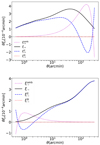 |
Fig. 1. Decomposition of the shear correlation functions ξ+(θ) (upper panel) and ξ−(ϑ) (lower panel) into pure E modes (dashed blue curves) and ambiguous modes (dotted magenta curves). The latter are quadratic functions of θ and 1/θ for ξ+ and ξ−, respectively. We note that |
At first sight, one might wonder that the ambiguous correlation function has a large amplitude. But what should be kept in mind is that the information of this function is contained solely in two numbers. In particular, as was shown in Asgari et al. (2012), they contain little cosmological information even if assumed to be solely due to E-mode shear.
Next, we turn to the “−” pure mode correlation functions. Using in turn Eqs. (24), (18), (3), and (44), we find
![$$ \begin{aligned} \xi _-^{E}(\vartheta )&+\xi _-^{B}(\vartheta ) ={\bar{\vartheta }^2\over B}\sum _{n=1}^\infty \tau _{+n}T_{-n}(\vartheta )\nonumber \\&={\bar{\vartheta }^2\over B}\sum _{n=1}^\infty \tau _{+n}\left[ T_{+n}(\vartheta ) +\int _{\vartheta _{\rm min}}^\vartheta {\mathrm{d}\theta \;\theta \over \vartheta ^2}\,T_{+n}(\theta )\,\left(4 -{12\theta ^2\over \vartheta ^2}\right) \right] \nonumber \\&=\xi _+(\vartheta )-S_+(\vartheta )+\int _{\vartheta _{\rm min}}^\vartheta {\mathrm{d}\theta \;\theta \over \vartheta ^2}\,\left[ \xi _+(\theta )-S_+(\theta ) \right] \,\left(4 -{12\theta ^2\over \vartheta ^2}\right) \nonumber \\&=\xi _+(\vartheta )+\int _{\vartheta _{\rm min}}^\vartheta {\mathrm{d}\theta \;\theta \over \vartheta ^2}\,\xi _+(\theta ) \,\left(4 -{12\theta ^2\over \vartheta ^2}\right) -V_+(\vartheta ) \;, \end{aligned} $$](/articles/aa/full_html/2022/08/aa42479-21/aa42479-21-eq81.gif)
where we have defined the function
and by using the definition (44) for S+, we obtain for the kernel K+ the following expression:
![$$ \begin{aligned} K_+&(\vartheta ,\theta )=H_+(\vartheta ,\theta )+\int _{\vartheta _{\rm min}}^\vartheta {\mathrm{d}\varphi \;\varphi \over \vartheta ^2}\,H_+(\varphi ,\theta ) \left(4-{12 \varphi ^2\over \vartheta ^2}\right) \nonumber \\&= {(1-B)^2\over 8 B^3} \Bigg \{ 3 (1-B)^2\left(\vartheta \over \bar{\vartheta }\right)^{-4} \left[ (1+B)^4-(1+4B+B^2)\left(\theta \over \bar{\vartheta }\right)^2 \right]\nonumber \\&\quad {+}\ \left(\vartheta \over \bar{\vartheta }\right)^{-2} \left[ 3(1+B)^2\left(\theta \over \bar{\vartheta }\right)^2-(3+6B+14 B^2+6B^3+3B^4) \right] \Bigg \} \nonumber \\&=\left(\bar{\vartheta }\over \vartheta \right)^2 H_-(\theta ,\vartheta ) \; . \end{aligned} $$](/articles/aa/full_html/2022/08/aa42479-21/aa42479-21-eq83.gif)
For the difference of the two “−” correlation functions we obtain
where
with the kernel function
![$$ \begin{aligned} K_-(\vartheta ,\theta )&={\bar{\vartheta }^4\over B}\sum _{\mu =a,b} T_{-\mu }(\vartheta ) T_{-\mu }(\theta )\nonumber \\&={\bar{\vartheta }^4(1-B^2)^2\over B\vartheta ^2\theta ^2} \Bigg \{{1\over 2}+{3\over 8B^2}\left[ 1+B^2-(1-B^2)^2\left(\bar{\vartheta }\over \vartheta \right)^2 \right]\nonumber \\&\quad \times \left[ 1+B^2-(1-B^2)^2\left(\bar{\vartheta }\over \theta \right)^2 \right] \Bigg \} \\&={(1-B^2)^2 \bar{\vartheta }^4\over \vartheta ^2 \theta ^2} H_+\left( {[1-B^2] \bar{\vartheta }^2\over \vartheta }, {[1-B^2] \bar{\vartheta }^2\over \theta }\right) \;.\nonumber \end{aligned} $$](/articles/aa/full_html/2022/08/aa42479-21/aa42479-21-eq86.gif)
Therefore,
![$$ \begin{aligned} \xi _-^{E}(\vartheta )&={1\over 2}\left[ \xi _+(\vartheta )+\xi _-(\vartheta ) +\int _{\vartheta _{\rm min}}^\vartheta {\mathrm{d}\theta \;\theta \over \vartheta ^2}\,\xi _+(\theta ) \left(4-{12\theta ^2\over \vartheta ^2}\right) \right] \nonumber \\&\quad {-}\ {1\over 2}\left[ V_+(\vartheta )+V_-(\vartheta ) \right]\;, \end{aligned} $$](/articles/aa/full_html/2022/08/aa42479-21/aa42479-21-eq87.gif)
![$$ \begin{aligned} \xi _-^{B}(\vartheta )&={1\over 2}\left[ \xi _+(\vartheta )-\xi _-(\vartheta ) +\int _{\vartheta _{\rm min}}^\vartheta {\mathrm{d}\theta \;\theta \over \vartheta ^2}\,\xi _+(\theta ) \left(4-{12\theta ^2\over \vartheta ^2}\right) \right] \nonumber \\&\quad {-}\ {1\over 2}\left[ V_+(\vartheta )-V_-(\vartheta ) \right]\;. \end{aligned} $$](/articles/aa/full_html/2022/08/aa42479-21/aa42479-21-eq88.gif)
The functions V±(ϑ) are of the form aϑ−2 + bϑ−4, and therefore correspond to shear correlations due to ambiguous modes. These are subtracted from the rest of the expression to yield pure E- and B-mode correlation functions. By subtracting Eq. (56) from Eq. (55), we obtain the second of Eqs. (22), with
An example for the decomposition of ξ− into E- and ambiguous modes is shown in the lower panel of Fig. 1. For large values of ϑ,  differs only little from ξ−, but their difference increases for smaller ϑ. In particular,
  has two roots in the interval ϑ ∈ [ϑmin, ϑmax].
We point out that pure-mode correlation functions equivalent to the foregoing ones were already defined in SEK. However, their expressions in terms of ξ± in SEK were considerably more complicated than the present ones, and therefore, they have not been applied to any data, as far as we know. Our choice of the orthonormality relation, which differs from the one in SEK, allowed us to obtain far more explicit expressions for the pure-mode shear correlation functions, and they are easily applicable to a set of measured ξ±, as we show in Sect. 4.
For completeness, we also note that in the case ϑmin = 0,  . In that case, B = 1, and thus T−a(ϑ)≡0 ≡ T−b(ϑ).
3.3. Comparison with “old” pure-mode shear correlation functions
3.3.1. General considerations
Previously, the CNPT correlation functions that were defined by Crittenden et al. (2002) and Schneider et al. (2002) also yield a mode separation; they are given in terms of the E- and B-mode convergence power spectra PE, B(ℓ) through
These functions can be expressed solely in terms of the shear correlation functions,
![$$ \begin{aligned} \xi _{E+}^\mathrm{CNPT}(\vartheta )&={1\over 2}\left[ \xi _+(\vartheta )+\xi _-(\vartheta )+\int _\vartheta ^\infty {\mathrm{d}\theta \over \theta }\; \xi _-(\theta )\left(4-{12\vartheta ^2\over \theta ^2}\right) \right] \;,\nonumber \\ \xi _{E-}^\mathrm{CNPT}(\vartheta )&={1\over 2}\left[ \xi _+(\vartheta )+\xi _-(\vartheta )+\int _0^\vartheta {\mathrm{d}\theta \;\theta \over \vartheta ^2}\; \xi _+(\theta )\left(4-{12\theta ^2\over \vartheta ^2}\right) \right] \;,\nonumber \\ \xi _{B+}^\mathrm{CNPT}(\vartheta )&={1\over 2}\left[ \xi _+(\vartheta )-\xi _-(\vartheta )-\int _\vartheta ^\infty {\mathrm{d}\theta \over \theta }\; \xi _-(\theta )\left(4-{12\vartheta ^2\over \theta ^2}\right) \right] \;, \\ \xi _{B-}^\mathrm{CNPT}(\vartheta )&={1\over 2}\left[ \xi _+(\vartheta )-\xi _-(\vartheta )+\int _0^\vartheta {\mathrm{d}\theta \;\theta \over \vartheta ^2}\; \xi _+(\theta )\left(4-{12\theta ^2\over \vartheta ^2}\right) \right] \;.\nonumber \end{aligned} $$](/articles/aa/full_html/2022/08/aa42479-21/aa42479-21-eq94.gif)
These can now be compared to the pure-mode correlation functions on a finite interval. We see that the functional form differs in two respects. First, the integrals over the correlation functions ξ± only extend over the finite interval for  , whereas they extend to either 0 or ∞ for
  . Second, in the
  a term that corresponds to the ambiguous modes is subtracted.
Another way to see the difference between the CNPT and the pure-mode correlation functions is by noting that

whereas the decomposition into the pure-mode correlation functions is given by Eq. (22).
The  are unobservable as they require a measurement of ξ± either down to zero separation or up to infinite separation; neither is possible. We note that the
  do not account for ambiguous modes, since for an infinite field, there are no ambiguous modes: a constant shear on an infinite field would violate the assumption of statistical isotropy of the random field (whereas on a collection of finite fields, the constant shear can have random magnitude and orientations for each field), and a linear shear field on an infinite field in addition would diverge (see the discussion in Appendix A). The ambiguous mode
  is due to the lack of information on ξ± for scales ϑ > ϑmax, whereas the
  is rooted in the missing information from scales ϑ < ϑmin.
We can check that the pure-mode shear correlation functions tend toward the CNPT correlation functions in the limit ϑmin → 0 or ϑmax → ∞. We consider first the “+” modes and let ϑmax → ∞, which also implies  and B → 1 such that
  . In this limit, the function H+(ϑ, θ) tends to a constant, and S+(ϑ)→0. Furthermore, H−(ϑ, θ)→0, due to the factors (1 − B)2 in Eq. (47); correspondingly, S−(ϑ)→0. Thus, in this limit, expressions (42) and (43) for
  converge to the corresponding ones in Eq. (59). For the “−” modes, we consider ϑmin → 0, implying B → 1. That means that K±(ϑ, θ)→0, and thus V±(ϑ)→0. Hence, we see that expressions (55) and (56) for
  converge to the corresponding ones in Eq. (59).
3.3.2. Comparison using SLICS
Asgari et al. (2019) modeled multiple data systematics that may exist in cosmic shear data. They applied these systematics to mock data from SLICS N-body simulations (see their Sect. 6 for details). Ten lines-of-sight were chosen and the measurements were applied to shape-noise-free mock data. Aside from the SEK COSEBIs they measured  from these simulations. Here we compare the pure mode correlation functions with their measurements.
Figure 2 compares the measured signal for both the pure-mode and the CNPT correlation functions. The results are shown for the mean of ten lines-of-sight. Here the mock data are free of systematic effects. The measurements are made for 50 logarithmic bins in θ. As can be seen, these two sets of correlation functions match at small separations, while they differ on larger scales; this is because ambiguous modes are not removed from  . In addition, a theoretical prediction for ξ− is used beyond θ = 300′, to calculate the integrals in Eq. (59). In particular, we can see that the pure mode
  closely recovers the zero B-mode prediction, in contrast to
  .
.
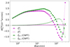 |
Fig. 2. Measured E- and B-mode correlation functions from SLICS simulations. Both E modes (squares) and B modes (crosses) are averaged over ten shape-noise-free lines-of-sight. The pure-mode correlation functions (magenta) are insensitive to information outside of the defined angular separation range, [0′.5, 300′]. The CNPT correlation functions (green) include ambiguous modes and information from outside of the measured range. |
We chose the point-spread function leakage, as modeled in Asgari et al. (2019, Sect. 5.1.1), as a test case. This systematics introduces both, artificial E and B modes. Figure 3 illustrates the E- and B-mode measurements in the left and right panels, respectively. In all cases the impact of the systematic is isolated via subtracting the fiducial no-systematic signal shown in Fig. 2. Again the old and new measurements match at small θ, while they differ at larger scales. The infinite upper bounds in Eq. (59) are more problematic here, since we do not have a theoretical prediction for this systematic effect. Using the pure-mode correlation functions allows us to isolate the scales where systematic effects create B modes without the need for extrapolating the measurements.
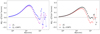 |
Fig. 3. Comparison between the CNPT and pure-mode correlation functions on systematic-induced mock data, averaged over ten shape-noise-free lines-of-sight. The point-spread function leakage as modeled by Asgari et al. (2019) is used here. The fiducial no-systematic signal is subtracted from the systematic-induced ones. All measurements are done for 50 logarithmic bins between 0.5 and 300 arcmin. |
3.4. Consistency checks
Having obtained explicit expressions for the pure-mode shear correlation functions, we now apply two checks on their consistency. First, we show explicitly that they are insensitive to ambiguous modes. Second, we show that for a pure E-mode shear field, the B-mode correlation functions vanish identically.
3.4.1. Insensitivity of  to ambiguous modes
As we mentioned before, some shear modes are neither E nor B modes, and they should not affect the  functions. For example, a constant shear field, with γ(θ) = γ0 leads to a pair of correlation functions ξ+(ϑ) = |γ0|2, ξ−(ϑ) = 0. In this particular case, we find from Eqs. (42), (43) that
![$$ \begin{aligned} \xi _+^{E}(\vartheta )=\xi _+^{B}(\vartheta )={1\over 2}\,\left[ \xi _+(\vartheta )-S_+(\vartheta ) \right]\;, \end{aligned} $$](/articles/aa/full_html/2022/08/aa42479-21/aa42479-21-eq113.gif)
with all other terms vanishing. However, since
S+(ϑ) = |γ0|2 = ξ+(ϑ) and  in this case. Hence, this ambiguous mode is filtered out. More generally, if we consider a linear shear field, for which
  and ξ−(ϑ) = 0, then again Eq. (61) holds, and since
![$$ \begin{aligned} \int _{\vartheta _{\rm min}}^{\vartheta _{\rm max}}{\mathrm{d}\theta \;\theta \over \bar{\vartheta }^2} \left[ a+b\left(\theta \over \bar{\vartheta }\right)^2 \right] H_+(\vartheta ,\theta )=a+b\left(\vartheta \over \bar{\vartheta }\right)^2 \;, \end{aligned} $$](/articles/aa/full_html/2022/08/aa42479-21/aa42479-21-eq117.gif)
we again obtain S+(ϑ) = ξ+(ϑ) and thus  .
.
3.4.2.  for pure E-mode shear
As an important consistency check of the foregoing discussion, we now want to show that the B-mode correlation functions  identically vanish if the shear field does not contain any B modes. In this case, the two correlation functions ξ± are related through
Hence, in the absence of B modes, Eq. (43) reduces to
In order to show that this vanishes, we first consider the term S+ and rewrite it with the help of Eq. (64),
![$$ \begin{aligned} S_+(\vartheta )&=\int _{\vartheta _{\rm min}}^{\vartheta _{\rm max}}{\mathrm{d}\theta \;\theta \over \bar{\vartheta }^2}\, \xi _+(\theta )\,H_+(\vartheta ,\theta )\nonumber \\&= \int _{\vartheta _{\rm min}}^{\vartheta _{\rm max}}{\mathrm{d}\theta \;\theta \over \bar{\vartheta }^2} \,H_+(\vartheta ,\theta ) \bigg [ \xi _-(\theta )+\int _\theta ^{\vartheta _{\rm max}}{\mathrm{d}\varphi \over \varphi }\xi _-(\varphi ) \left(4-{12\theta ^2\over \varphi ^2}\right)\nonumber \\&\quad {+}\ \int _{\vartheta _{\rm max}}^\infty {\mathrm{d}\varphi \over \varphi }\xi _-(\varphi ) \left(4-{12\theta ^2\over \varphi ^2}\right)\bigg ] \nonumber \\&= \int _{\vartheta _{\rm min}}^{\vartheta _{\rm max}}{\mathrm{d}\theta \;\theta \over \bar{\vartheta }^2}\, H_+(\vartheta ,\theta )\,\xi _-(\theta ) \\&\quad {+}\ \int _{\vartheta _{\rm min}}^{\vartheta _{\rm max}}{\mathrm{d}\varphi \over \varphi }\;\xi _-(\varphi ) \int _{\vartheta _{\rm min}}^\varphi {\mathrm{d}\theta \;\theta \over \bar{\vartheta }^2}\,H_+(\vartheta ,\theta )\, \left(4-{12\theta ^2\over \varphi ^2}\right)\nonumber \\&\quad {+}\ \int _{\vartheta _{\rm min}}^{\vartheta _{\rm max}}{\mathrm{d}\theta \;\theta \over \bar{\vartheta }^2}\,H_+(\vartheta ,\theta ) \int _{\vartheta _{\rm max}}^\infty {\mathrm{d}\varphi \over \varphi }\xi _-(\varphi ) \left(4-{12\theta ^2\over \varphi ^2}\right) \;,\nonumber \end{aligned} $$](/articles/aa/full_html/2022/08/aa42479-21/aa42479-21-eq123.gif)
where the function H+(ϑ, θ) is given by Eq. (46), and in the second step we have changed the order of integration, subject to the constraint ϑmin ≤ θ ≤ φ ≤ ϑmax. Thus, we have rewritten S+ solely in terms of ξ−, as are the other terms in Eq. (65). One finds that
which shows that the final term in Eq. (66) cancels the first term on the r.h.s. of Eq. (65). Hence,  does not have any contributions of ξ− from outside the considered interval. The remaining terms are
![$$ \begin{aligned} 2\xi ^\mathrm{B}_+(\vartheta )&=\int _{\vartheta _{\rm min}}^{\vartheta _{\rm max}}{\mathrm{d}\theta \over \theta }\;\xi _-(\theta )\; \bigg [\left(\theta \over \bar{\vartheta }\right)^2H_+(\vartheta ,\theta ) \nonumber \\&\quad {+}\ \int _{\vartheta _{\rm min}}^\theta {\mathrm{d}\varphi \;\varphi \over \bar{\vartheta }^2} \,H_+(\vartheta ,\varphi )\left(4-{12\varphi ^2\over \theta ^2}\right)-H_-(\vartheta ,\theta )\bigg ] \;, \end{aligned} $$](/articles/aa/full_html/2022/08/aa42479-21/aa42479-21-eq126.gif)
where the function H−(ϑ, θ) is given by Eq. (47). Carrying out the φ integral, one can show that the bracket in Eq. (68) vanishes identically, and thus  (ϑ)≡0 in the absence of B modes.
Similarly, we find from Eqs. (56) and (64) in the case of vanishing B modes
![$$ \begin{aligned} 2\xi ^{B}_-(\vartheta )&=\int _{\vartheta _{\rm min}}^{\vartheta _{\rm max}}{\mathrm{d}\theta \;\theta \over \bar{\vartheta }^2}\,\xi _+(\theta ) \, \left[ K_-(\vartheta ,\theta )-K_+(\vartheta ,\theta ) \right] \nonumber \\&\quad {-}\ \int _0^{\vartheta _{\rm min}}{\mathrm{d}\theta \;\theta \over \vartheta ^2}\,\xi _+(\theta )\left(4-{12\theta ^2\over \vartheta ^2}\right) \\&\quad {+}\ \int _{\vartheta _{\rm min}}^{\vartheta _{\rm max}}{\mathrm{d}\theta \;\theta \over \bar{\vartheta }^2}\,K_-(\vartheta ,\theta ) \int _0^\theta {\mathrm{d}\varphi \;\varphi \over \theta ^2}\,\xi _+(\varphi ) \left(4-{12\varphi ^2\over \theta ^2}\right) \;. \nonumber \end{aligned} $$](/articles/aa/full_html/2022/08/aa42479-21/aa42479-21-eq128.gif)
The last integral is then split into one from 0 to ϑmin and one from ϑmin to θ. For the former, we note the result that
so that the corresponding θ integral just cancels the second term in Eq. (69). Hence,  contains no contribution from scales outside the angular interval considered. For the θ integration of the second φ integral, we change the order of integration, subject to ϑmin ≤ φ ≤ θ ≤ ϑmax, to get
![$$ \begin{aligned} 2\xi ^{B}_-(\vartheta )&=\int _{\vartheta _{\rm min}}^{\vartheta _{\rm max}}{\mathrm{d}\theta \;\theta \over \bar{\vartheta }^2}\,\xi _+(\theta ) \, \Bigg [ K_-(\vartheta ,\theta )-K_+(\vartheta ,\theta ) \nonumber \\&\quad {+}\ \int _\theta ^{\vartheta _{\rm max}}{\mathrm{d}\varphi \over \varphi }\;K_-(\vartheta ,\varphi ) \left(4-{12\theta ^2\over \varphi ^2}\right) \Bigg ] \;. \end{aligned} $$](/articles/aa/full_html/2022/08/aa42479-21/aa42479-21-eq131.gif)
One can show that the term in the bracket is identically zero, which shows that  ≡0 for the case that the shear field has no B-mode contribution.
3.5. Relation to the power spectrum
We now consider the relation between the shear power spectra and the pure-mode shear correlation functions. The ξ±(ϑ) are related to the E- and B-mode power spectra PE(ℓ) and PB(ℓ) by
![$$ \begin{aligned} \xi _+(\vartheta )&=\int _0^\infty {\mathrm{d}\ell \;\ell \over 2\pi }\;\mathrm{J}_0(\ell \vartheta )\, \left[ P_{E}(\ell )+P_{B}(\ell ) \right]\;, \nonumber \\ \xi _-(\vartheta )&=\int _0^\infty {\mathrm{d}\ell \;\ell \over 2\pi }\;\mathrm{J}_4(\ell \vartheta )\, \left[ P_{E}(\ell )-P_{B}(\ell ) \right]\; . \end{aligned} $$](/articles/aa/full_html/2022/08/aa42479-21/aa42479-21-eq133.gif)
Expressions (42), (43), (55), (56) show that  are linear in the ξ± and hence can be expressed in the form
![$$ \begin{aligned} \xi _\pm ^{E}(\vartheta )&=\int _0^\infty {\mathrm{d}\ell \;\ell \over 2\pi }\,\left[ W_{\pm {E}}^{E}(\ell ,\vartheta )\,P_{E}(\ell )+W_{\pm {B}}^{E}(\ell ,\vartheta )P_{B}(\ell ) \right]\;, \nonumber \\ \xi _\pm ^{B}(\vartheta )&=\int _0^\infty {\mathrm{d}\ell \;\ell \over 2\pi }\,\left[ W_{\pm {E}}^{B}(\ell ,\vartheta )\,P_{E}(\ell )+W_{\pm {B}}^{B}(\ell ,\vartheta )P_{B}(\ell ) \right] \;. \end{aligned} $$](/articles/aa/full_html/2022/08/aa42479-21/aa42479-21-eq135.gif)
We start with  , for which the coefficients read
![$$ \begin{aligned}&W_{+{E}}^{E}(\ell ,\vartheta )={1\over 2}\Biggl [ \mathrm{J}_0(\ell \vartheta )+\mathrm{J}_4(\ell \vartheta ) +\int _\vartheta ^{\vartheta _{\rm max}}{\mathrm{d}\theta \over \theta }\;\mathrm{J}_4(\ell \theta )\, \left(4-{12 \vartheta ^2\over \theta ^2}\right) \nonumber \\&\quad {-}\ \int _{\vartheta _{\rm min}}^{\vartheta _{\rm max}}{\mathrm{d}\theta \;\theta \over \bar{\vartheta }^2}\, \mathrm{J}_0(\ell \theta )\,H_+(\vartheta ,\theta ) -\int _{\vartheta _{\rm min}}^{\vartheta _{\rm max}}{\mathrm{d}\theta \over \theta }\;\mathrm{J}_4(\ell \theta )\, H_-(\vartheta ,\theta ) \Biggr ] \;, \nonumber \\&W_{+{B}}^{E}(\ell ,\vartheta )={1\over 2}\Biggl [ \mathrm{J}_0(\ell \vartheta )-\mathrm{J}_4(\ell \vartheta ) -\int _\vartheta ^{\vartheta _{\rm max}}{\mathrm{d}\theta \over \theta }\;\mathrm{J}_4(\ell \theta )\, \left(4-{12 \vartheta ^2\over \theta ^2}\right) \nonumber \\&\quad {-}\ \int _{\vartheta _{\rm min}}^{\vartheta _{\rm max}}{\mathrm{d}\theta \;\theta \over \bar{\vartheta }^2}\, \mathrm{J}_0(\ell \theta )\,H_+(\vartheta ,\theta ) +\int _{\vartheta _{\rm min}}^{\vartheta _{\rm max}}{\mathrm{d}\theta \over \theta }\;\mathrm{J}_4(\ell \theta )\, H_-(\vartheta ,\theta ) \Biggr ] \;. \nonumber \end{aligned} $$](/articles/aa/full_html/2022/08/aa42479-21/aa42479-21-eq137.gif)
We expect that the latter coefficient vanishes, since the pure E-mode correlation function should not depend on the B-mode power spectrum. Indeed, it can be shown that  . By adding the previous two equations, we can simplify the expression for
  to
to
![$$ \begin{aligned}&W_{+{E}}^{E}(\ell ,\vartheta )=\mathrm{J}_0(\ell \vartheta ) -\int _{\vartheta _{\rm min}}^{\vartheta _{\rm max}}{\mathrm{d}\theta \;\theta \over \bar{\vartheta }^2}\, \mathrm{J}_0(\ell \theta )\, H_+(\vartheta ,\theta ) \nonumber \\&{=}\ \mathrm{J}_0(\ell \vartheta )-{(1+B)\over 4 B^2 \ell \bar{\vartheta }} \left[ 3\left(\vartheta \over \bar{\vartheta }\right)^2-(3-2B+3B^2) \right] \mathrm{J}_1(\ell {\vartheta _{\rm max}})\nonumber \\&\quad {-}\ {(1-B)\over 4 B^2 \ell \bar{\vartheta }} \left[ 3\left(\vartheta \over \bar{\vartheta }\right)^2-(3+2B+3B^2) \right] \mathrm{J}_1(\ell {\vartheta _{\rm min}})\nonumber \\&\quad {+}\ {3 \over 4B^3 (\ell \bar{\vartheta })^2}\,\left[ \left(\vartheta \over \bar{\vartheta }\right)^2-(1+B^2) \right] \\&\quad {\times }\ \left[ (1+B)^2\, \mathrm{J}_2(\ell {\vartheta _{\rm max}}) -(1-B)^2\,\mathrm{J}_2(\ell {\vartheta _{\rm min}}) \right] \;. \nonumber \end{aligned} $$](/articles/aa/full_html/2022/08/aa42479-21/aa42479-21-eq140.gif)
We first note that the function  does not only depend on the product ℓϑ, as was the case for the corresponding filter for ξ+. Since the pure-mode correlation functions depend on the angular interval ϑmin ≤ ϑ ≤ ϑmax, the filter
  has an explicit dependence on the interval boundaries, expressed through B,
  and the arguments of the Bessel functions. The additional terms in
  filter out the ambiguous modes. In fact, since for small ℓ,
  , low-ℓ modes in the power spectrum are strongly suppressed.
The foregoing fact is an important observation. The filter that relates ξ+ to the power spectra is J0(ℓϑ), which tends to unity as ℓ → 0. Hence, ξ+ is very sensitive to small-ℓ power (i.e., to large-scale modes). The fact that the filter  has a leading ℓ4 dependence shows that the sensitivity of ξ+ to large-scale modes is due solely to the ambiguous modes in ξ+.
Turning to  , it is straightforward to see that
  and
and  . Thus, the pure B-mode correlation function is independent of the E-mode power spectrum, and the relation between
  and PB is the same as between
  and PE.
The filter functions for  are
are
![$$ \begin{aligned}&W_{-{E/B}}^{E}(\ell ,\vartheta )={1\over 2}\Biggl [ \mathrm{J}_0(\ell \vartheta )\pm \mathrm{J}_4(\ell \vartheta ) + \int _{\vartheta _{\rm min}}^\vartheta {\mathrm{d}\theta \;\theta \over \vartheta ^2}\,\mathrm{J}_0(\ell \theta ) \left(4-{12\theta ^2\over \vartheta ^2}\right) \nonumber \\&{-}\ \int _{\vartheta _{\rm min}}^{\vartheta _{\rm max}}{\mathrm{d}\theta \;\theta \over \bar{\vartheta }^2}\, \mathrm{J}_0(\ell \theta )\,K_+(\vartheta ,\theta ) \mp \int _{\vartheta _{\rm min}}^{\vartheta _{\rm max}}{\mathrm{d}\theta \;\theta \over \bar{\vartheta }^2}\;\mathrm{J}_4(\ell \theta )\, K_-(\vartheta ,\theta ) \Biggr ] \;, \nonumber \end{aligned} $$](/articles/aa/full_html/2022/08/aa42479-21/aa42479-21-eq153.gif)
where the upper (lower) signs apply for  (
( ). We find that
  , as expected, that is, the B-mode power does not contribute to the pure E-mode correlation function
  . Taking the sum of the two filter functions, we find that
![$$ \begin{aligned}&W_{-{E}}^{E}(\ell ,\vartheta )=\mathrm{J}_0(\ell \vartheta ) +\int _{\vartheta _{\rm min}}^\vartheta {\mathrm{d}\theta \;\theta \over \vartheta ^2}\,\mathrm{J}_0(\ell \theta ) \left(4-{12\theta ^2\over \vartheta ^2}\right) \nonumber \\&\qquad \qquad \ \ \,{-}\ \int _{\vartheta _{\rm min}}^{\vartheta _{\rm max}}{\mathrm{d}\theta \;\theta \over \bar{\vartheta }^2}\, \mathrm{J}_0(\ell \theta )\,K_+(\vartheta ,\theta ) \nonumber \\&{=}\ \mathrm{J}_4(\ell \vartheta ) +{(1-B^2)\over 4 B^2 \ell \bar{\vartheta }} \left[ a_{-1}^\mathrm{min}\mathrm{J}_1(\ell {\vartheta _{\rm min}}) +a_{-1}^\mathrm{max}\mathrm{J}_1(\ell {\vartheta _{\rm max}}) \right] \\&\ \ {+}\ {3(1-B^2)^2\over 4 B^3 (\ell \bar{\vartheta })^2} \left[ a_{-2}^\mathrm{min}\mathrm{J}_2(\ell {\vartheta _{\rm min}}) +a_{-2}^\mathrm{max}\mathrm{J}_2(\ell {\vartheta _{\rm max}}) \right] \;, \nonumber \end{aligned} $$](/articles/aa/full_html/2022/08/aa42479-21/aa42479-21-eq158.gif)
where the coefficients are
![$$ \begin{aligned} a_{-1}^\mathrm{min}&=(1+B)\left[ 3(1-B^2)^2\left(\vartheta \over \bar{\vartheta }\right)^{-4} -(3-2B+3B^2)\left(\vartheta \over \bar{\vartheta }\right)^{-2} \right] \;, \nonumber \\ a_{-1}^\mathrm{max}&=(1-B)\left[ 3(1-B^2)^2\left(\vartheta \over \bar{\vartheta }\right)^{-4} -(3+2B+3B^2)\left(\vartheta \over \bar{\vartheta }\right)^{-2} \right] \;,\nonumber \\ a_{-2}^\mathrm{min}&=(1+B)^2(1-4B+B^2)\left(\vartheta \over \bar{\vartheta }\right)^{-4} -(1-B^2)\left(\vartheta \over \bar{\vartheta }\right)^{-2} \;, \\ a_{-2}^\mathrm{max}&=(1+B^2)\left(\vartheta \over \bar{\vartheta }\right)^{-2} -(1-B)^2(1+4B+B^2)\left(\vartheta \over \bar{\vartheta }\right)^{-4} \;.\nonumber \end{aligned} $$](/articles/aa/full_html/2022/08/aa42479-21/aa42479-21-eq159.gif)
Finally, we find  , again as expected since the correlation function
  should not depend on the E-mode power spectrum, and
  . Thus, of the eight filter functions
  , four are identically zero, and the remaining four are pairwise identical, so that only the two given in Eqs. (74) and (75) need to be evaluated.
We note that as ϑmin → 0, ϑmax → ∞,  and
and  , due to the behavior of the Bessel functions for small and large arguments. Hence, in this case the relation between the pure-mode shear correlation functions and the power spectra reduces to that of the CNPT correlation functions.
Finally, from the decomposition (22) of the correlation functions and the results of this subsection, we find the relation between the ambiguous modes and the power spectra,
![$$ \begin{aligned} \xi _+^\mathrm{amb}(\vartheta )&=\int {\mathrm{d}\ell \over 2\pi }\, \left[ \mathrm{J}_0(\ell \vartheta )-W_{+E}^{E}(\ell ,\vartheta ) \right]\, \left[ P_{E}(\ell )+P_{B}(\ell ) \right]\;,\nonumber \\ \xi _-^\mathrm{amb}(\vartheta )&=\int {\mathrm{d}\ell \over 2\pi }\, \left[ \mathrm{J}_4(\ell \vartheta )-W_{-E}^{E}(\ell ,\vartheta ) \right]\, \left[ P_{E}(\ell )-P_{B}(\ell ) \right]\;. \end{aligned} $$](/articles/aa/full_html/2022/08/aa42479-21/aa42479-21-eq166.gif)
Given that both of the  are characterized by only two coefficients, it is obvious that one can find many combinations of E- and B-mode power spectra for which these coefficients are the same. Therefore, these ambiguous mode correlation functions can result from different combinations of E and B modes. We give some specific examples for this in Appendix A.3.
4. KiDS-1000 measurements
4.1. Data description
The Kilo Degree Survey is designed with weak gravitational lensing applications in mind. Its data, therefore, benefit from high-quality images in the r-band (mean seeing of 0.7 arcsec), which is used for the shape measurements (Giblin et al. 2021). In addition, all galaxies have matched depth images in optical, ugri, and near-infrared photometric bands, ZYJHKs. The five near-infrared bands are observed by the VISTA Kilo-degree INfrared Galaxy (VIKING) survey (Edge et al. 2013). These nine bands are used to estimate photometric redshifts for all galaxies that contribute to the cosmic shear signal. The fourth KiDS data release includes 1006 square degrees of images (Kuijken et al. 2019). The data are divided into five tomographic bins before 2PCFs are measured for the 15 distinct combinations of redshift bins3. The redshift distribution for each tomographic bin is calibrated using KiDS+VIKING-like observations of fields containing spectroscopic samples (Hildebrandt et al. 2021).
The theoretical predictions were calculated with the KiDS Cosmology Analysis Pipeline4 (KCAP), which is built from the modular cosmology pipeline COSMOSIS5 (Zuntz et al. 2015). The primordial power spectrum was estimated using the CAMB Boltzmann code (Lewis et al. 2000). Its nonlinear evolution was calculated via the augmented halo model approach of Mead et al. (2015), which also accounts for the impact of baryon feedback from active galactic nuclei. We modeled the intrinsic alignments of galaxies with the nonlinear linear alignment (NLA) model of Bridle & King (2007, see also Hirata & Seljak 2004) and used a modified Limber approximation (LoVerde & Afshordi 2008) to project the three-dimensional power spectra into two dimensions, PE(ℓ). This was then used to make predictions for the pure mode correlation functions and the new dimensionless COSEBIs.
4.2. COSEBIs and pure-mode correlations for KiDS-1000
We calculated the new dimensionless logarithmic COSEBIs (see Appendix B) by integrating over the measured ξ±6. The pure-mode correlation functions were determined by integrating over the ξ±, according to the relations given in Sect. 3.2. As a consistency check, we also calculated  using Eqs. (23) and (24), using the first 20 COSEBIs modes. We found that the sums in Eqs. (23) and (24) converge to the previous result after about the first five COSEBI modes.
Figures 4–6 display the measured dimensionless COSEBIs,  and
and  for the angular separation range of 0.5 to 300 arcmin. In these figures, the error bars are drawn from the diagonal of their respective covariance matrix. Each panel belongs to a pair of redshift bins. The theoretical curves were calculated using the best fitting flat ΛCDM cosmology to the KiDS-1000 cosmic shear data (SEK COSEBIs; Asgari et al. 2021) whose parameter values are given in Table 1. Although not listed here we also fix the mean redshift displacement parameters to their best fitting values as estimated in Asgari et al. (2021). In all cases, the theory values are connected to each other for ease of comparison, although they are all discrete with the exception of the unbinned theory curves (blue) in Fig. 5. For COSEBIs this is true by definition, while for
  the binning of the data requires the theoretical predictions to also be binned (orange dashed curves).
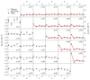 |
Fig. 4. Dimensionless logarithmic COSEBI (see Appendix B) measurements from KiDS-1000 data. The E and B modes are shown in the top and bottom triangles, respectively. Each panel depicts results for a pair of redshift bins, z − ij. The solid red curves correspond to the best fitting model to the SEK COSEBIs as analyzed in Asgari et al. (2021, compare with their Fig. 3). The B modes are consistent with zero (p-value = 0.36) and the best-fit model describes the data very well (p-value = 0.2). We note that the COSEBI modes are discrete and the points are connected to one another for visual aid. |
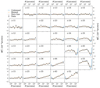 |
Fig. 5. KiDS-1000 pure E-mode correlation functions. Top and bottom panels: |


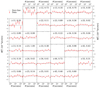 |
Fig. 6. KiDS-1000 pure B-mode correlation functions. |


Fiducial cosmological parameters.
4.3. Covariances and Fisher analysis
We first derived the covariance matrix for the new COSEBIs using the methodology detailed in Joachimi et al. (2021) and Appendix A of Asgari et al. (2020). The corresponding correlation matrix is shown in the left panel of Fig. 7 and compared to the correlation matrix for the SEK COSEBIs shown on the right. As can be seen, the dimensionless COSEBIs are considerably less correlated, making them more mutually independent.
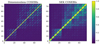 |
Fig. 7. Correlation matrices for new (left) and old (right) logarithmic COSEBIs. Here we illustrate the correlation matrices for the first five COSEBI modes. Each five-by-five block shows the values for one pair of redshift bins, starting with the lowest bins at the bottom-left corner. |
We then estimated the covariance matrices for the pure-mode correlation functions, making use of the linear relation between them and the COSEBIs given by Eqs. (23) and (24). The correlation coefficients are shown in Fig. 8 for  .
.
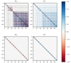 |
Fig. 8. Correlation coefficients for pure-mode correlation functions. They are shown for the autocorrelations of |


Although the theoretical curves are not fitted to the data in Figs. 4 and 5, we see that they describe the data very well7. We estimated the goodness-of-fit using the probability of exceeding the measured χ2 (i.e., the p-value). Following Joachimi et al. (2021) we assume that the effective number of free parameters is 4.5 and set the degrees of freedom to the number of data points, minus 4.5. We then find that all p-values are above 0.09 (p-values for each data vector are reported in the caption of their figure). This is to be expected as the fit is done to the SEK COSEBIs (p-value = 0.16), which separate E and B modes on the same angular range. Figure 6 and the bottom panels of Fig. 4, depict the B-mode signals. We find that the B modes are consistent with zero in all cases and all p-values are above 0.1. We also report the p-values for individual pairs of redshift bins in Fig. 6, which can be compared with the results of Giblin et al. (2021) who used SEK COSEBIs to determine the significance of B modes in KiDS-1000 data. We note that, as demonstrated in Asgari et al. (2019), the significance of the B modes has a nontrivial dependence on the way the data are binned and, equivalently, on the number of COSEBI modes that are used8, as well as on the types of systematic effects that exist in the data. While certain systematics produce E and B modes on similar angular separations (see for example the impact of point-spread-function leakage in Fig. 3), others such as a CCD-chip bias that produces a repeating pattern in the images (see for example Asgari et al. 2019, regular pattern Figs. 9 and 10), show a different scale dependence for E and B modes. Therefore, similar to COSEBIs here we recommend to use multiple binning schemes to test the significance of B modes. In fact, we found similar trends to Giblin et al. (2021) depending on the number of θ bins. When we divide the [0′.5, 300′] range into 20 θ bins we found that bin 55 has the smallest p-value = 0.04, whereas dividing the same range into five bins resulted in smaller p-values for redshift bin combinations 22 and 35. Nevertheless, all p-values are above the 0.01 threshold and thus we conclude that the B modes are insignificant. We also found that by increasing the number of θ bins, the p-values resulting from  and
and  become very similar, confirming that these two functions contain the same information.
We compare the information content of the pure mode correlation function,  with the SEK COSEBIs, in Fig. 9. We use a Fisher formalism and assume the fiducial values in Table 1 for model parameters. As was shown in Asgari et al. (2021), we expect to have meaningful constraints only for the structure growth parameter S8 and the amplitude of the intrinsic alignments AIA. Therefore, we fixed all other parameters and only show the 1σ and 2σ contours for S8 and AIA. We see that the information content of
  and COSEBIs is identical, and conclude that there is no extra cosmological information to be gained from the pure-mode correlation functions. This is also true when we compare the dimensionless and SEK COSEBIs Fisher matrices. This is to be expected, as both methods make use of the E-mode information that is available in the given angular interval. With the Fisher analysis we can also estimate the expected errors on the measured parameters. We find that the error on S8 is 0.014 and on AIA is 0.274, both are slightly smaller than the full likelihood analysis of Asgari et al. (2021), as expected.
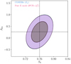 |
Fig. 9. Fisher matrix forecast for KiDS-1000. The SEK COSEBIs (blue) are compared with |

5. Summary and discussion
In this paper we have derived pure-mode shear correlation functions that can be obtained from the measured shear correlations, ξ±(ϑ), on a finite interval, 0 < ϑmin ≤ ϑ ≤ ϑmax < ∞. This was achieved by redefining the orthonormality relation of COSEBIs, which allowed us to construct two complete sets of orthonormal weight functions, T±μ(ϑ), on this finite interval; explicit expressions for these new weight functions are given in Appendix B. Two of these weight functions correspond to ambiguous modes, and with the remaining ones, the mode-separating COSEBIs were defined. Owing to the completeness of these function sets, we were able to decompose the shear correlation functions into their E- and B-mode correlations,  , and their contribution by ambiguous modes (see Eq. 22). These different components can be straightforwardly determined from the ξ±(ϑ) measured on a finite interval, in contrast to the CNPT correlation functions (see Sect. 3.3), which require extrapolation or the modeling of ξ± for separations smaller or larger than where measurements of ξ± are available. Hence, there is no longer any reason to use these CNPT correlation functions. Only in the limit of ϑmin → 0 and ϑmax → ∞ do they agree with mode-separating ones.
These new correlation functions allow the study of E- and B-mode second-order shear as a function of angular scale. Hence, they should serve as a diagnostic for the angular dependence of potential B modes in a survey. To illustrate this, we applied the pure-mode correlation functions to simulation data, without and with systematics added, and compared the results with our earlier analysis (Asgari et al. 2019).
We applied the newly constructed dimensionless COSEBIs to the KiDS-1000 tomographic cosmic shear data set, for which we also computed the pure-mode shear correlation functions. Calculating the covariance of the COSEBIs and the binned  , we have shown that their measured values are fully consistent with the best fitting model parameters obtained in Asgari et al. (2021), exhibiting only very small differences in the p-values. Using the Fisher analysis, we also showed that the results on the two parameters best constrained by the cosmic shear data (S8 and AIA) are indistinguishable between the COSEBIs and the pure-mode correlation functions – as was to be expected. The discrete nature of the COSEBIs makes them the more convenient quantities for a cosmological analysis.
In Appendix A we provide a few illustrative examples of ambiguous modes in the shear correlation function, that is, modes that cannot be uniquely attributed either to E or B modes. Incorporation of such modes into a cosmological analysis carries the risk that they are affected by a contribution coming from B modes, and hence the analysis may be biased. We therefore caution against the use of ambiguous modes when deriving constraints on model parameters; instead, employing COSEBIs for that purpose avoids this potential trap. We note that the sensitivity of ξ+(ϑ) to low-ℓ power, due to the filter J0(ℓϑ) relating them, is solely due to ambiguous modes; the corresponding filter function for the pure-mode correlation has an ℓ4 dependence for ℓ → 0.
As was shown in Asgari et al. (2012), if one assumes that the ambiguous modes are pure E modes, then they contain additional cosmological information – this corresponds to the case termed “full COSEBIs” in Asgari et al. (2012). The relative amount of information in these ambiguous modes depends on the angular range ϑmin to ϑmax, and presumably on the number of cosmological parameters. However, as was made clear above, from the measurement of the correlation functions on this finite interval, one cannot tell whether these ambiguous modes are pure E modes or whether B modes are mixed in. We therefore strongly advise against the use of ambiguous modes for cosmological parameter inference.
The same statement holds for the correlation functions ξ±; to use them for cosmological parameter estimates, one needs to (implicitly) assume that they are pure E-mode functions, which cannot be verified from a measurement on a finite angular separation interval. Thus, such estimates may contain an unknown level of systematics due to B modes that remain undetected by the COSEBIs but are hidden in the ambiguous modes.
Finally, we show in Appendix C that the COSEBIs defined on a subinterval of the original one can be obtained as linear combinations of the original COSEBIs. This was to be expected since these original COSEBIs contain the full E and B mode-separable information about second-order shear statistics. We thus conclude that it suffices to consider the COSEBIs on the full angular range where the ξ± are measured without needing to consider subintervals. The lack of localized information in the individual COSEBIs is remedied by the use of the pure-mode shear correlation functions derived here.
A specific example for EE and BB are the aperture dispersions,  and
and  , considered in Schneider et al. (2002); for them, ϑmin = 0 and ϑmax = 2θ. In that case, the corresponding function T−(ϑ) is nonnegative, and hence does not obey conditions (5) – see Fig. 1 in Schneider et al. (2002).
We refer the reader to Asgari et al. (2017) for details on this conversion from ξ± to COSEBIs.
In principle, as mentioned before, the dimensionless COSEBIs and the pure-mode correlation functions should yield exactly the same result as using the SEK COSEBIs, as all these quantities contain the same information. In practice, however, the results will slightly differ, due to the use of a finite number of COSEBI modes and a finite number of ϑ bins for the correlation functions.
Acknowledgments
We acknowledge the constructive comments by the anonymous referee which led to an improvement of the presentation. This work was supported by the Deutsche Forschungsgemeinschaft with the grant SCHN342-13 and the Heisenberg grant Hi 1495/5-1, the European Research Council under grants number 647112 and 770935, by an STFC Ernest Rutherford Fellowship (project reference ST/S004858/1), by the Max Planck Society and the Alexander von Humboldt Foundation in the framework of the Max Planck-Humboldt Research Award endowed by the Federal Ministry of Education and Research ERC with the Consolidator Grant No. 770935, by the Vici grant 639.043.512, financed by the Netherlands Organisation for Scientific Research (NWO), by the Royal Society and Imperial College, by the CMS-CSST-2021-A01, NSFC of China under grant 11973070, the Shanghai Committee of Science and Technology grant No.19ZR1466600 and Key Research Program of Frontier Sciences, CAS, grant No. ZDBS-LY-7013, and the Leverhulme Trust. Based on observations made with ESO Telescopes at the La Silla Paranal Observatory under programme IDs 177.A-3016, 177.A-3017, 177.A-3018 and 179.A-2004, and on data products produced by the KiDS consortium. The KiDS production team acknowledges support from: Deutsche Forschungsgemeinschaft, ERC, NOVA and NWO-M grants; Target; the University of Padova, and the University Federico II (Naples). Author contributions: All authors contributed to the development and writing of this paper. The authorship list is given in two groups: the lead authors (PS,MA,YNJ) followed by an alphabetical group that covers those who have either made a significant contribution to the data products, or to the scientific analysis.
References
- Aihara, H., Arimoto, N., Armstrong, R., et al. 2018, PASJ, 70, S4 [NASA ADS] [Google Scholar]
- Albrecht, A., Bernstein, G., Cahn, R., et al. 2006, ArXiv eprints [ArXiv:astro-ph/0609591] [Google Scholar]
- Asgari, M., & Heymans, C. 2019, MNRAS, 484, L59 [NASA ADS] [CrossRef] [Google Scholar]
- Asgari, M., & Schneider, P. 2015, A&A, 578, A50 [NASA ADS] [CrossRef] [EDP Sciences] [Google Scholar]
- Asgari, M., Schneider, P., & Simon, P. 2012, A&A, 542, A122 [NASA ADS] [CrossRef] [EDP Sciences] [Google Scholar]
- Asgari, M., Heymans, C., Blake, C., et al. 2017, MNRAS, 464, 1676 [NASA ADS] [CrossRef] [Google Scholar]
- Asgari, M., Heymans, C., Hildebrandt, H., et al. 2019, A&A, 624, A134 [NASA ADS] [CrossRef] [EDP Sciences] [Google Scholar]
- Asgari, M., Tröster, T., Heymans, C., et al. 2020, A&A, 634, A127 [NASA ADS] [CrossRef] [EDP Sciences] [Google Scholar]
- Asgari, M., Lin, C.-A., Joachimi, B., et al. 2021, A&A, 645, A104 [NASA ADS] [CrossRef] [EDP Sciences] [Google Scholar]
- Becker, M. R. 2013, MNRAS, 435, 1547 [CrossRef] [Google Scholar]
- Becker, M. R., & Rozo, E. 2016, MNRAS, 457, 304 [NASA ADS] [CrossRef] [Google Scholar]
- Blandford, R. D., Saust, A. B., Brainerd, T. G., & Villumsen, J. V. 1991, MNRAS, 251, 600 [NASA ADS] [Google Scholar]
- Blazek, J. A., MacCrann, N., Troxel, M. A., & Fang, X. 2019, Phys. Rev. D, 100, 103506 [NASA ADS] [CrossRef] [Google Scholar]
- Bridle, S., & King, L. 2007, New J. Phys., 9, 444 [Google Scholar]
- Bunn, E. F. 2011, Phys. Rev. D, 83, 083003 [Google Scholar]
- Crittenden, R. G., Natarajan, P., Pen, U.-L., & Theuns, T. 2002, ApJ, 568, 20 [NASA ADS] [CrossRef] [Google Scholar]
- DES Collaboration (Abbott, T. M. C., et al.) 2021, Phys. Rev. D, 105, 023520 [Google Scholar]
- Deshpande, A. C., Kitching, T. D., Cardone, V. F., et al. 2020, A&A, 636, A95 [NASA ADS] [CrossRef] [EDP Sciences] [Google Scholar]
- Edge, A., Sutherland, W., Kuijken, K., et al. 2013, The Messenger, 154, 32 [NASA ADS] [Google Scholar]
- Erben, T., Hildebrandt, H., Miller, L., et al. 2013, MNRAS, 433, 2545 [Google Scholar]
- Gatti, M., Sheldon, E., Amon, A., et al. 2021, MNRAS, 504, 4312 [NASA ADS] [CrossRef] [Google Scholar]
- Giahi-Saravani, A., & Schäfer, B. M. 2014, MNRAS, 437, 1847 [CrossRef] [Google Scholar]
- Giblin, B., Heymans, C., Asgari, M., et al. 2021, A&A, 645, A105 [NASA ADS] [CrossRef] [EDP Sciences] [Google Scholar]
- Harnois-Déraps, J., Amon, A., Choi, A., et al. 2018, MNRAS, 481, 1337 [Google Scholar]
- Heydenreich, S., Schneider, P., Hildebrandt, H., et al. 2020, A&A, 634, A104 [NASA ADS] [CrossRef] [EDP Sciences] [Google Scholar]
- Heymans, C., White, M., Heavens, A., Vale, C., & van Waerbeke, L. 2006, MNRAS, 371, 750 [Google Scholar]
- Heymans, C., Van Waerbeke, L., Miller, L., et al. 2012, MNRAS, 427, 146 [Google Scholar]
- Heymans, C., Grocutt, E., Heavens, A., et al. 2013, MNRAS, 432, 2433 [Google Scholar]
- Heymans, C., Tröster, T., Asgari, M., et al. 2021, A&A, 646, A140 [NASA ADS] [CrossRef] [EDP Sciences] [Google Scholar]
- Hilbert, S., Hartlap, J., White, S. D. M., & Schneider, P. 2009, A&A, 499, 31 [NASA ADS] [CrossRef] [EDP Sciences] [Google Scholar]
- Hilbert, S., Xu, D., Schneider, P., et al. 2017, MNRAS, 468, 790 [Google Scholar]
- Hildebrandt, H., Viola, M., Heymans, C., et al. 2017, MNRAS, 465, 1454 [Google Scholar]
- Hildebrandt, H., van den Busch, J. L., Wright, A. H., et al. 2021, A&A, 647, A124 [EDP Sciences] [Google Scholar]
- Hinton, S. R. 2016, J. Open Source Software, 1, 00045 [NASA ADS] [CrossRef] [Google Scholar]
- Hirata, C. M., & Seljak, U. 2004, Phys. Rev. D, 70, 063526 [Google Scholar]
- Joachimi, B., Semboloni, E., Hilbert, S., et al. 2013, MNRAS, 436, 819 [Google Scholar]
- Joachimi, B., Cacciato, M., Kitching, T. D., et al. 2015, Space Sci. Rev., 193, 1 [Google Scholar]
- Joachimi, B., Lin, C. A., Asgari, M., et al. 2021, A&A, 646, A129 [NASA ADS] [CrossRef] [EDP Sciences] [Google Scholar]
- Kaiser, N. 1992, ApJ, 388, 272 [Google Scholar]
- Kaiser, N. 1998, ApJ, 498, 26 [NASA ADS] [CrossRef] [Google Scholar]
- Kilbinger, M. 2018, ArXiv e-prints [arXiv:1807.08249] [Google Scholar]
- Kilbinger, M., Schneider, P., & Eifler, T. 2006, A&A, 457, 15 [NASA ADS] [CrossRef] [EDP Sciences] [Google Scholar]
- Kitching, T. D., Paykari, P., Hoekstra, H., & Cropper, M. 2019, Open J. Astrophys., 2, 5 [CrossRef] [Google Scholar]
- Krause, E., & Hirata, C. M. 2010, A&A, 523, A28 [NASA ADS] [CrossRef] [EDP Sciences] [Google Scholar]
- Kuijken, K., Heymans, C., Hildebrandt, H., et al. 2015, MNRAS, 454, 3500 [Google Scholar]
- Kuijken, K., Heymans, C., Dvornik, A., et al. 2019, A&A, 625, A2 [NASA ADS] [CrossRef] [EDP Sciences] [Google Scholar]
- Lewis, A., Challinor, A., & Lasenby, A. 2000, ApJ, 538, 473 [Google Scholar]
- LoVerde, M., & Afshordi, N. 2008, Phys. Rev. D, 78 [CrossRef] [Google Scholar]
- Mandelbaum, R. 2018, ARA&A, 56, 393 [Google Scholar]
- Mead, A. J., Peacock, J. A., Heymans, C., Joudaki, S., & Heavens, A. F. 2015, MNRAS, 454, 1958 [NASA ADS] [CrossRef] [Google Scholar]
- Peacock, J. A., Schneider, P., Efstathiou, G., et al. 2006, ESA-ESO Working Group on "Fundamental Cosmology", Tech. rep. [Google Scholar]
- Schneider, P. 1996, MNRAS, 283, 837 [Google Scholar]
- Schneider, P., & Kilbinger, M. 2007, A&A, 462, 841 [NASA ADS] [CrossRef] [EDP Sciences] [Google Scholar]
- Schneider, P., & Seitz, C. 1995, A&A, 294, 411 [NASA ADS] [Google Scholar]
- Schneider, P., van Waerbeke, L., Jain, B., & Kruse, G. 1998, MNRAS, 296, 873 [NASA ADS] [CrossRef] [Google Scholar]
- Schneider, P., van Waerbeke, L., & Mellier, Y. 2002, A&A, 389, 729 [NASA ADS] [CrossRef] [EDP Sciences] [Google Scholar]
- Schneider, P., Eifler, T., & Krause, E. 2010, A&A, 520, A116 [NASA ADS] [CrossRef] [EDP Sciences] [Google Scholar]
- Sevilla-Noarbe, I., Bechtol, K., Carrasco Kind, M., et al. 2021, ApJS, 254, 24 [NASA ADS] [CrossRef] [Google Scholar]
- Shapiro, C. 2009, ApJ, 696, 775 [NASA ADS] [CrossRef] [Google Scholar]
- Troxel, M. A., & Ishak, M. 2015, Phys. Rep., 558, 1 [NASA ADS] [CrossRef] [Google Scholar]
- Vale, C., Hoekstra, H., van Waerbeke, L., & White, M. 2004, ApJ, 613, L1 [NASA ADS] [CrossRef] [Google Scholar]
- White, M. 2005, Astropart. Phys., 23, 349 [NASA ADS] [CrossRef] [Google Scholar]
- Wolfram, S. 1991, Mathematica: a System for Doing Mathematics by Computer, (Addison-Wesley Pub. Co.) [Google Scholar]
- Zuntz, J., Paterno, M., Jennings, E., et al. 2015, Astron. Comput., 12, 45 [NASA ADS] [CrossRef] [Google Scholar]
Appendix A: Shear fields from ambiguous modes
In this appendix, we consider ambiguous modes of the shear field in more detail. This will be done in different ways. First, we give several examples of shear fields that cannot uniquely be assigned to either E-mode or B-mode shear. We then show that a statistical ensemble of such shear fields give rise to the ambiguous modes in the shear 2PCFs. Finally, we show that ambiguous modes in the shear correlation functions can be caused by various combinations of E- and B-mode power spectra.
A.1. Ambiguous shear fields
Following Crittenden et al. (2002) and Schneider et al. (2002), we formally describe a general shear field by a superposition of E and B modes, by defining the complex deflection potential ψ(θ) = ψE(θ)+iψB(θ), where ψE/B are real functions. The corresponding convergence is then obtained from the Poisson equation, κ(θ) = κE(θ)+iκB(θ) = (1/2)∇2ψ(θ). The shear field is given by
![$$ \begin{aligned} \gamma =\gamma _1+\mathrm{i}\gamma _2= \left[ {\psi _{,11}^\mathrm{E}-\psi ^\mathrm{E}_{,22}\over 2} -\psi ^\mathrm{B}_{,12} \right] +\mathrm{i}\left[ \psi ^\mathrm{E}_{,12} +{\psi _{,11}^\mathrm{B} -\psi ^\mathrm{B}_{,22}\over 2} \right]\;, \end{aligned} $$](/articles/aa/full_html/2022/08/aa42479-21/aa42479-21-eq194.gif)
where subscripts following a comma denote partial derivatives with respect to θi. We consider the following combinations of second derivatives of the shear,
Thus, we see that a shear field that does not contain a B-mode component satisfies Cc ≡ 0, whereas one that has no E-mode contribution satisfies Cg ≡ 0. In the following we provide examples for shear fields for which Cg ≡ 0 ≡ Cc, and thus result either from an E- or a B-mode deflection potential.
The first example is one where the deflection potential is a polynomial of order 3. Since constant and linear terms in ψ do not cause any shear, we write
This yields the linear shear field
It is obvious that such a linear shear field can be equally obtained from E-mode and B-mode deflection potentials, and thus such a shear field corresponds to an ambiguous mode. Obviously, Cg ≡ 0 ≡ Cc for such a field.
A less trivial example is obtained by considering axi-symmetric shear fields of the form
where here we use complex notation for a vector θ (i.e., θ = θ1 + iθ2), and the asterisk denotes complex conjugation. The term θ/θ* = e2iφ, where φ is the polar angle of θ, is just a phase factor. Such a shear field is tangential to the origin at every point, and can be generated by an axi-symmetric mass distribution κE or, equivalently, an axi-symmetric deflection potential ψE. From Eq. (A.2) we find that Cc(θ)≡0 for this shear field, independent of the function F. For Cg, we find
![$$ \begin{aligned} C_{\rm g}({\boldsymbol{\theta }})=-4\left[ 2 F^{\prime }\left(|{\boldsymbol{\theta }}|^2\right)+|{\boldsymbol{\theta }}|^2 F^{\prime \prime }\left(|{\boldsymbol{\theta }}|^2\right) \right]\;, \end{aligned} $$](/articles/aa/full_html/2022/08/aa42479-21/aa42479-21-eq199.gif)
which is nonzero in general. However, for F(X) = const. or F(X)∝X−1, Cg also vanishes. We consider the latter case first: it corresponds to
the shear field of a point mass. Curiously, we can also get the same shear field from a B-mode potential. Indeed, we let

and then we get
in agreement with Eq. (A.7), for any value of f. This indeed is a curious result, stating that a pure tangential shear field – the “classical” case of an E-mode field – can be obtained from a B-mode potential. Putting this is different words: If we take the tangential shear field (A.7) and rotate the shear at every position by 45 degree (equivalent to multiplying the shear by a factor i), then we get the classical case of a B-mode shear field. However, this rotated field can be obtained from a pure E-mode potential ψE = −arctan(θ2/θ1). We should point out, though, that the arctan(θ2/θ1) is not defined on the θ2-axis where it jumps from −π/2 to π/2, and thus the rosette-like shear field cannot be obtained from a globally defined E-mode potential (or convergence). But if one considers the shear field on any finite region not crossing the θ2-axis, one cannot tell whether the shear field (A.7) is due to an E or a B mode.9
Likewise, the shear field

which is a tangential shear field with an amplitude independent of radius |θ|, can be generated both by an E- and B-mode deflection potential: letting

leads to the shear field (A.10) for any f.
A.2. Shear correlation functions from ambiguous shear fields
We now consider isotropic statistical ensembles of ambiguous shear fields and consider the resulting shear correlation functions. For that, we consider the shear on two points on the θ1-axis, at θ = ( ± ϑ/2, 0), so that ξ+(ϑ) = ⟨γ(−ϑ/2)γ*(ϑ/2)⟩ and ξ−(ϑ) = ⟨γ(−ϑ/2)γ(ϑ/2)⟩.10 Starting with the linear shear field, we consider an ensemble of such fields, and write the shear in complex notation as

where, due to the fact that the shear is a spin-2 field, the coefficients Gn are spin-n quantities that, under a rotation of the coordinate frame, transform as Gn → Gn e−niφ. Accordingly,
![$$ \begin{aligned} \gamma (-\vartheta /2)\,\gamma (\vartheta /2)&=G_2^2-(G_1^2+G_3^2+2G_1 G_3)\vartheta ^2/4\;, \nonumber \\ \gamma (-\vartheta /2)\,\gamma ^*(\vartheta /2)&=| G_2 |^2 -\left(| G_1 |^2+| G_3 |^2+G_1G_3^*+G_1^*G_3\right) \vartheta ^2/4 \nonumber \\&+\left[ G_2\left(G_1^*+G_3^*\right)-G_2^*\left(G_1+G_3\right) \right]\vartheta /2 \;. \end{aligned} $$](/articles/aa/full_html/2022/08/aa42479-21/aa42479-21-eq206.gif)
If we now consider a statistical ensemble of such linear fields, we have to average over the coefficients. Statistical isotropy then implies that  for m ≠ n, as well ⟨GnGn⟩ = 0, due to phase averaging over these spin ≠ 0 quantities. Therefore,
which corresponds to the ambiguous modes discussed in Sect. A.1.
We next turn to the shear field caused by an ensemble of point masses. Specifically, we consider a circular region of radius Θ in which there are N point masses at locations θi and relative masses mi, with mean mass ⟨m⟩. At the end we consider the limit Θ → ∞, N → ∞, such that the mean number density  is constant. The shear field then reads
We assume the positions θi of the point masses to be random inside the circle. Therefore, the expectation value of the product γ(−ϑ/2)γ(ϑ/2) is
![$$ \begin{aligned} \xi _-(\vartheta )&=\left\langle \gamma (-\vartheta /2)\gamma (\vartheta /2) \right\rangle = \left[ \prod _{n=1}^N{1\over \pi \Theta ^2}\int _0^\Theta \mathrm{d}|\theta _n|\;|\theta _n| \int _0^{2\pi }\mathrm{d}\varphi _n \right] \nonumber \\&\times \sum _{i,j=1}^N \left( {m_i\over (\theta _i -\vartheta /2)^2} {m_j\over (\theta _j + \vartheta /2)^2}\right)^* \;. \end{aligned} $$](/articles/aa/full_html/2022/08/aa42479-21/aa42479-21-eq211.gif)
We now split the sum into terms i ≠ j and those with i = j. In the former case, each term of the sum depends only on two θn, and the rest integrate out to unity. Those off-diagonal terms yield
where
We can now calculate the inner integral. For that, we let u = eiφ, dφ = −i du/u, so the φ integral becomes
where the integral extends over the unit circle. This integral was calculated in Schneider (1996) to yield
![$$ \begin{aligned} {4 \pi \over \vartheta ^2}\left[ 2 \mathrm{H}\left({\vartheta \over 2}-\theta \right)- {\vartheta \over 2}\,\delta _{\rm D}\left(\theta -{\vartheta \over 2}\right) \right]\;. \end{aligned} $$](/articles/aa/full_html/2022/08/aa42479-21/aa42479-21-eq215.gif)
so that I(ϑ/2) = 0 for Θ > ϑ/2. Thus, the off-diagonal terms in Eq. (A.16) do not contribute to ξ−. In fact, I(θ) is the shear caused by a uniform disk of matter of radius Θ, and it is well known that such a disk causes no shear for Θ > θ.
This leaves us with the diagonal terms i = j,
Employing the residue theorem, we note three poles at u1 = 0, u2 = ϑ/(2θ), and u3 = −ϑ/(2θ), with Res(u1) = 16/ϑ4, Res(u2) = Res(u3) = − 8/ϑ4. The latter two poles lie inside the unit circle for θ > ϑ/2, and for this case, the contour integral vanishes. Thus, we find
corresponding to one of the ambiguous modes discussed in Sect. A.1. Repeating the calculations for the correlation ξ+(ϑ), we find that the non-diagonal terms in the double sum vanish as well, and we are left with
The integrand in the contour integral has poles at u1 = ϑ/(2θ) and u2 = −2θ/ϑ, and the corresponding residue are Res(u1) = − 16(ϑ2 − 4θ2)/(ϑ2 + 4θ2)3 and Res(u2) = 16(ϑ2 − 4θ2)/(ϑ2 + 4θ2)3. The former (latter) pole is inside the unit circle for θ > ϑ/2 (θ < ϑ/2). Performing the θ integral then yields ξ+(ϑ) = 0.
In fact, this result could have been anticipated: the convergence power spectrum for a random field of point masses is a constant, and the correlation function of the convergence vanishes for any finite separation. But the shear correlation function ξ+ is identical to the convergence correlation, so that ξ+(ϑ) = 0 for ϑ > 0. Furthermore, for a constant power spectrum, the second of Eqs. (72) shows that ξ−(ϑ)∝ϑ−2. We also note that the first of Eqs. (64) implies that ξ−(ϑ)∝ϑ−2 yields ξ+(ϑ) = 0.
We have been unable to find an analogous example of a shear field that can be obtained from a deflection potential and which yields a ξ−(ϑ)∝ϑ−4 correlation. However, if we drop the requirement that the shear field can be obtained from a potential – for example, the shear field is due to some systematics unrelated to the lensing effect – then one can construct such examples. If we consider the spin-3 field
then we find that Cc ≡ 0 ≡ Cg if F(X) satisfies the differential equation X2F″+6XF′+6F = 0. The two independent solutions, F ∝ X−2 and F ∝ X−3, then lead to shear fields of the form γ(θ)∝θ3/|θ|4 and γ(θ)∝θ3/|θ|6. Choosing the latter and constructing a random field with it, in the same way as we did above for the point masses, we find indeed that ξ−(ϑ)∝ϑ−4.
A.2. Ambiguous modes in ξ± and their relation to power spectra
We consider here the relation between shear correlation function and the underlying power spectra, and provide examples of correlations functions that can be derived equally well from an E- or B-mode power spectrum, or a linear combination of both.
We start by noting that the relation between the correlation functions and the E- and B-mode power spectra, PE(ℓ) and PB(ℓ), respectively, is given by Eq. (72). If the correlation functions are known for all ϑ, one can invert these relations and get a unique decomposition into E and B modes,
![$$ \begin{aligned} P_{\rm E}(\ell )&=\pi \int _0^\infty \mathrm{d}\vartheta \;\vartheta \, \left[ \xi _+(\vartheta )\,\mathrm{J_0}(\ell \vartheta )+\xi _-(\vartheta )\,\mathrm{J_4}(\ell \vartheta ) \right] \;, \nonumber \\ P_{\rm B}(\ell )&=\pi \int _0^\infty \mathrm{d}\vartheta \;\vartheta \, \left[ \xi _+(\vartheta )\,\mathrm{J_0}(\ell \vartheta )-\xi _-(\vartheta )\,\mathrm{J_4}(\ell \vartheta ) \right] \;, \end{aligned} $$](/articles/aa/full_html/2022/08/aa42479-21/aa42479-21-eq220.gif)
but on a finite interval of separations, this decomposition is not possible. As an example, we consider the power spectrum11
![$$ \begin{aligned} P_0(\ell ) ={2\pi \vartheta _2\over \ell ^2 \vartheta _0^2} \left[ \ell \left(\vartheta _0^2\, \xi _0+\vartheta _2^2\, \xi _2\right)\mathrm{J}_1(\ell \vartheta _2) -2\vartheta _2\, \xi _2 \,\mathrm{J}_2(\ell \vartheta _2) \right] \;, \end{aligned} $$](/articles/aa/full_html/2022/08/aa42479-21/aa42479-21-eq221.gif)
where ϑ2 > ϑmax, and ϑ0 is a fiducial angular scale, and let the E- and B-mode power spectra be PE(ℓ) = fP0(ℓ), PB(ℓ) = (1 − f)P0(ℓ). Then we find from Eq. (72) that
for ϑ < ϑ2, and thus for ϑ ≤ ϑmax, valid for any value of f. Hence, we can obtain the pair of correlation functions (A.27) for any distribution of power on the E- and B-mode power spectra. Therefore, we have the two ambiguous modes ξ+ = const. and ξ+ ∝ ϑ2. We note that these modes are ambiguous only on a finite interval. For ϑ > ϑ2, ξ+ = 0, but ξ− ≠ 0, and in particular, ξ− ∝ (2f − 1). Hence, if we had information about ξ± on all scales, we could determine the parameter f, and the mode assignment would be unique.
Similarly, we consider the power spectrum
![$$ \begin{aligned} P_0(\ell )={2\pi \vartheta _0^2\over \ell ^2\vartheta _1^3} \left[ 2\xi _{-2}\vartheta _1 \mathrm{J}_2(\ell \vartheta _1) +\ell \left(\xi _{-2}\vartheta _1^2+\xi _{-4}\vartheta _0^2\right)\mathrm{J}_3(\ell \vartheta _1) \right] \;, \end{aligned} $$](/articles/aa/full_html/2022/08/aa42479-21/aa42479-21-eq223.gif)
where ϑ1 < ϑmin. We now distribute this power as PE(ℓ) = (1 + f)P0(ℓ), PB(ℓ) = fP0(ℓ) over E- and B modes, and then find from Eq. (72) that
which is valid for ϑ > ϑ1 and thus for ϑ ≥ ϑmin. We note that this pair of correlation functions are independent of f, and thus valid for any distribution of the power P0 over E and B modes. Hence, this is a second pair of ambiguous modes, namely ξ+ = 0, and ξ− ∝ ϑ−2 and ξ− ∝ ϑ−4. Whereas ξ−(ϑ) = 0 for ϑ < ϑ1, ξ+(ϑ)≠0 for smaller ϑ, and in particular it is proportional to (1 + 2f). Thus, again, these modes are ambiguous only on a finite interval.
For the more general case, we assume that the correlation functions  ,
,  are written as a sum of two terms, where the ones with a “0” superscript do not yield any ambiguous modes
  . On the other hand, we assume that Δξ+(ϑ) is purely ambiguous (i.e., of the form Δξ+(ϑ) = ξ0 + ξ2(ϑ/ϑ0)2 on the finite interval ϑmin ≤ ϑ ≤ ϑmax) but has an arbitrary functional form for larger and smaller separations. The coefficients ξ0, 2 are directly related to the Ea, b + Ba, b defined above. From Eq. (A.25), we then find

We again distribute the power over modes in the form ΔPE(ℓ) = fP0(ℓ), ΔPB(ℓ) = (1 − f)P0(ℓ), and then calculate Δξ−(ϑ) on the finite interval,
![$$ \begin{aligned} \Delta \xi _-(\vartheta )&=(2f-1)\int _0^\infty \mathrm{d}\ell \;\ell \,\mathrm{J}_4(\ell \vartheta ) \int _0^\infty \mathrm{d}\theta \;\theta \,\mathrm{J}_0(\ell \theta )\,\Delta \xi _+(\theta ) \nonumber \\&= (2f-1)\Bigg \{\Delta \xi _+(\vartheta ) +\int _0^{\vartheta _{\rm min}}\!\mathrm{d}\theta \;\theta \, \Delta \xi _+(\theta )\left({4\over \vartheta ^2}-{12\theta ^2\over \vartheta ^4}\right)\nonumber \\&\quad + \int _{\vartheta _{\rm min}}^\vartheta \mathrm{d}\theta \;\theta \,\left[ \xi _0+\xi _2\left(\vartheta \over \vartheta _0\right)^2 \right]\left({4\over \vartheta ^2}-{12\theta ^2\over \vartheta ^4}\right) \Bigg \} \\&= (2f-1)\Bigg \{{1\over \vartheta ^2} \left[ 4\int _0^{\vartheta _{\rm min}}\!\!\!\!\mathrm{d}\theta \;\theta \,\Delta \xi _+(\vartheta ) -2\vartheta _{\rm min}^2\xi _0-{\vartheta _{\rm min}^4\over \vartheta _0}\,\xi _2 \right]\nonumber \\&+{1\over \vartheta ^4} \left[ 12\int _0^{\vartheta _{\rm min}}\!\mathrm{d}\theta \;\theta ^3\,\Delta \xi _+(\vartheta ) +3\vartheta _{\rm min}^4\xi _0+{2\vartheta _{\rm min}^6\over \vartheta _0^2}\xi _2 \right]\Bigg \} \;,\nonumber \end{aligned} $$](/articles/aa/full_html/2022/08/aa42479-21/aa42479-21-eq229.gif)
where we made use of the relation

where δD and H denote the Dirac delta “ function” and the Heaviside step function, respectively. We see that Δξ−(ϑ) only contains ambiguous modes inside the finite interval and that their amplitudes depend on the integral of Δξ+ over scales below ϑmin; in other words, the amplitudes are assumed to be unmeasured. Because of this, the fraction f of B-mode power attributed to the Δξ± cannot be determined. We can go through the analogous exercise to fix Δξ− and calculate Δξ+, which then only contains ambiguous modes with an amplitude that depends on f and moments of ξ− taken over scales larger than ϑmax.
Appendix B: A new set of COSEBIs
The μ = n coefficients in Eq. (17) define the COSEBIs. These COSEBIs depend on the choice of the weight functions T±n(ϑ). We point out that the T±n(ϑ) used in this paper differ from those in SEK in their dimensions: whereas in SEK, these filter functions were chosen to be dimensionless, we chose them here to have dimension (angle)−2, as can be seen from Eq. (6). Correspondingly, the COSEBIs defined here are dimensionless, whereas they have dimension (angle)2 in SEK. We think the current choice is more natural than the earlier one.
Furthermore, our orthonormality relation (6) differs from that of SEK through the factor ϑ in the integral. This new definition allowed us to show that the T−n(ϑ) also form an orthonormal basis, which they do not with the orthonormality relation used in SEK.
In SEK, we constructed two sets of functions T±n(ϑ), one polynomials in ϑ and the other polynomials in ln(ϑ), termed linear and logarithmic COSEBIs, respectively. The latter were shown to be more convenient, in that fewer COSEBI modes are needed to extract the full cosmological information contained in mode-separable correlation functions.
B.1. Linear COSEBIs
We consider the case of polynomial COSEBIs first, for which we transform the interval ϑmin ≤ ϑ ≤ ϑmax onto the interval −1 ≤ x ≤ 1 via
We then set  . Since
  , we then see from Eqs. (6) and (14) that the t±n(x) obey the orthonormality relations
This equation also motivates the pre-factor in the orthonormality relation (6). Furthermore, the constraints (4) are translated into
The functions  are then calculated from
We constructed a set of polynomial functions t+n(x) obeying the orthonormality relation (B.2) and the constraints (B.3), where t+n(x) is a polynomial of (n + 1)-th order, given by
![$$ \begin{aligned} t_{+1}(x)&={(5-B^2)\,P_2(x)-3 B \,P_1(x)+B^2 \,P_0(x)\over \sqrt{10-6B^2}} \;, \nonumber \\ t_{+n}(x)&=\left[ 2 (n+2)\, B\, P_{n+1}\left(1\over B\right)\, P_{n+2}\left(1\over B\right) \right]^{-1/2} \\&\times \sum _{k=0}^{n+1}(-1)^{k} (2k+1)\, P_k\left(1\over B\right)\, P_k(x)\quad \mathrm{for}\quad n\ge 2 \;. \nonumber \end{aligned} $$](/articles/aa/full_html/2022/08/aa42479-21/aa42479-21-eq238.gif)
The sign of the t+n(x) has been chosen such that t+n(−1) > 0, implying T+n(ϑmin) > 0. In order to show the validity of this result, we first consider, for n ≥ 2, the expression
![$$ \begin{aligned} (1+Bx)&\sum _{k=0}^{n+1}(-1)^{k} (2k+1) P_k\left(1\over B\right) P_k(x)\nonumber \\&= B\sum _{k=0}^{n+1}(-1)^{k}\Bigg \{{2k+1\over B} P_k\left(1\over B\right) P_k(x) \\&+P_k\left(1\over B\right)\left[ (k+1)P_{k+1}(x)+k P_{k-1}(x) \right]\Bigg \} \;,\nonumber \end{aligned} $$](/articles/aa/full_html/2022/08/aa42479-21/aa42479-21-eq239.gif)
where we used the recursion relation for Legendre polynomials, Pk. Changing the summation index for the last two terms as k → k ± 1 and applying the recursion relation for Legendre polynomials again, this time for the Pk(1/B), we see that only two terms survive, and we obtain
![$$ \begin{aligned} (1+&Bx) \sum _{k=0}^{n+1}(-1)^{k} (2k+1) P_k\left(1\over B\right) P_k(x) \\&= (-1)^{n+1} (n+2) B \left[ P_{n+1}\left(1\over B\right)P_{n+2}(x)+P_{n+2} \left(1\over B\right)P_{n+1}(x) \right] \;.\nonumber \end{aligned} $$](/articles/aa/full_html/2022/08/aa42479-21/aa42479-21-eq240.gif)
Therefore, we find that, for n ≥ 2,
![$$ \begin{aligned} (1+Bx)\,t_{+n}(x)&=(-1)^{n+1}\sqrt{(n+2)B\over 2P_{n+1}(1/B) P_{n+2}(1/B)} \nonumber \\ \times&\left[ P_{n+1}\left(1\over B\right)P_{n+2}(x) +P_{n+2}\left(1\over B\right)P_{n+1}(x) \right] \;. \end{aligned} $$](/articles/aa/full_html/2022/08/aa42479-21/aa42479-21-eq241.gif)
Using the orthogonality relation of the Legendre polynomials, it is then straightforward to show that the orthonormality relation (B.2) is satisfied for m, n ≥ 2. Furthermore, since (1 + Bx)t+n for n ≥ 2 contains no term Pk(x) with k ≤ 2, the orthogonality relation is clearly valid for m = 1, n ≥ 2. Finally, it is easy to see that conditions (B.3) are satisfied for n ≥ 2, and for n = 1, it can be shown from straightforward integration. Hence, the system (B.5) forms the set of polynomial weight functions we were looking for.
It should be stressed that these functions are easy to calculate: for a given survey setup, one needs to calculate the Pk(1/B) only once, and the Pn(x) are easily obtainable from the recursion relation of the Legendre polynomials. Whereas it is possible in principle to obtain explicit expressions for the corresponding functions t−n(x), this may not be needed: since the calculation of COSEBIs requires the calculation of the ξ± and the T−n at a large number of ϑ-values (see Asgari & Schneider 2015), it is probably computationally more efficient to evaluate the integrals in Eq. (B.4) using very small increments in the upper bound x.
B.2. Logarithmic COSEBIs
The roots of the polynomial weight functions T+n(ϑ) are fairly uniformly distributed over the interval ϑmin < ϑ < ϑmax. The shear correlation functions ξ±(ϑ) vary more strongly for smaller ϑ than for larger ϑ, and therefore are expected to contain more (cosmological) information on these smaller scales. Therefore, it is useful to consider a set of weight functions T+n(ϑ) that also show more structure on smaller scales, as done before in SEK. We let
so that the functions t+n(z) are defined for 0 ≤ z ≤ ln(ϑmax/ϑmin) = zm. The constraints (4) and the orthonormality relation (6) then read in terms of the t+n:
We now choose the t+n(z) to be polynomials of order n + 1, and write them in the form
The equations (B.10) then lead to a linear system of equations for the coefficients cnk, as was shown in SEK. Indeed, this system is very similar to the corresponding one in SEK, and differs only in the definition of the orthonormality relation for the T+n. Hence, we refer the reader to SEK for details of the method how the solution for the cnk is obtained. As was mentioned there, one needs the cnk to have very high numerical precision, in particular for large values of ϑmax/ϑmin. However, if we write the polynomials in the form
then a moderate precision for the roots rni is sufficient. As an example, for ϑmax/ϑmin = 400 and eight significant digits of the rni, the orthonormality relations for the first 20 T+n are satisfied to better than 10−18. In Fig. B.1, we display a Mathematica (Wolfram 1991) program that calculates the roots rni.
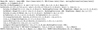 |
Fig. B.1. Mathematica (Wolfram 1991) program to calculate the roots in Eq. (B.12). They are stored with eight significant digits in the lower-left half of the table ROOTS, and the table NORM contains the normalization coefficients, Nn |
An expression for the corresponding function ![$ T_{-n}({\vartheta})=t_{-n}[\ln({\vartheta}/{{{\vartheta}_{\text{ min}}}})]/\bar{\vartheta}^2 $](/articles/aa/full_html/2022/08/aa42479-21/aa42479-21-eq246.gif) can then be calculated from Eq. (3), yielding
can then be calculated from Eq. (3), yielding
![$$ \begin{aligned} t_{-n}(z)=t_{+n}(z)+\int _0^z\mathrm{d}y\; t_{+n}(y)\left[ 4 \mathrm{e}^{2(y-z)} -12\mathrm{e}^{4(y-z)} \right]\;. \end{aligned} $$](/articles/aa/full_html/2022/08/aa42479-21/aa42479-21-eq247.gif)
Hence, the t−n can be easily calculated as numerical integrals over the t+n in the form (B.12).
The COSEBIs are related to the underlying power spectrum by the integral
where the weight function Wn is given by
These weight functions thus describe the sensitivity of the COSEBIs to the power spectrum. As an example, we plot in Fig. B.2 the function W5(ℓ) and compare it to the corresponding one of the COSEBIs defined in SEK, in both cases for the logarithmic weight functions. As can be seen, the “new” W5 is significant nonzero over a somewhat broader range in ℓ. It is this feature that makes the new COSEBIs less correlated than the old ones, as shown in Fig. 7. On the other hand, the wider ℓ-range may lead to an increase in the sensitivity of the COSEBIs to different baryonic feedback effects, compared to that of the SEK COSEBIs (see Asgari et al. 2020), which shall be explored in future work.
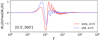 |
Fig. B.2. Comparison between the new dimensionless (solid red) and the old SEK (dashed blue) COSEBIs. We show the form of the fifth COSEBI weight function, W5(ℓ). Each curve is normalized with respect to its maximum value. We chose an angular separation interval of 0.5 to 300 arcminutes to define the weights. |
In particular, it must be stressed that the information content of the SEK COSEBIs and the dimensionless COSEBIs are exactly the same, if their full (infinite) sets are considered; in fact, one can transform one set into the other. The difference in the properties illustrated in Figs. 7 and B.2 are not due to the different orthonormality relations, but due to the specific choice of polynomial weight functions T+n(ϑ). Different sets of weight functions may be constructed, for example to make the first N of the Wn(ℓ) more localized and thus potentially less sensitive to baryonic effects.
Appendix C: COSEBIs on a subinterval
In this section we consider the relation between the COSEBIs on a subinterval  , and the original ones on [ϑmin, ϑmax], where
  . We denote with B′ and
  the relative width and the mean angle inside the subinterval. Furthermore, we denote by
  the basis functions on the subinterval, which have a support on this subinterval. The coefficients
  , defined in analogy with Eqs. (19) and (20), are then obtained from the correlation functions ξ± by
where we used representation (18) of the correlation function and defined
Using the relation between the τ±n and the COSEBIs En, Bn, we obtain
![$$ \begin{aligned} E_\mu ^{\prime }&={\tau ^{\prime }_{+\mu }+\tau ^{\prime }_{-\mu }\over 2}={1\over 2}\sum _\nu \left[ \left(\mathcal{T}^+_{\mu \nu }+\mathcal{T}^-_{\mu \nu }\right)E_\nu +\left(\mathcal{T}^+_{\mu \nu }-\mathcal{T}^-_{\mu \nu }\right)B_\nu \right] \;,\nonumber \\ B_\mu ^{\prime }&={\tau ^{\prime }_{+\mu }-\tau ^{\prime }_{-\mu }\over 2}={1\over 2}\sum _\nu \left[ \left(\mathcal{T}^+_{\mu \nu }-\mathcal{T}^-_{\mu \nu }\right)E_\nu +\left(\mathcal{T}^+_{\mu \nu }+\mathcal{T}^-_{\mu \nu }\right)B_\nu \right] \;.\nonumber \end{aligned} $$](/articles/aa/full_html/2022/08/aa42479-21/aa42479-21-eq257.gif)
We now look at some properties of the transfer matrices 𝒯±. Since the functions  and T−n are related to
  and T+n though the transformation (9), we can apply the Lemma in Sect. 2 and obtain from Eq. (C.2) that

Furthermore, for ν = a, b, the functions T+ν(ϑ) are of the form x0 + x2ϑ2. From the analog of conditions (4) for the  functions, we then infer that
Similarly, for ν = a, b, the functions T−ν(ϑ) are of the form x2ϑ−2 + x4ϑ−4, so that the condition (5) yields
Together, we than find that
This result then shows that the E- and B-mode COSEBIs on the subinterval can be calculated from the E- and B-mode COSEBIs on the original angular interval. The transfer matrix 𝒯+ depends on the choice of basis functions; in general we expect that in order to obtain  to a given accuracy, one needs to use En’s up to significantly larger n. However, subdividing the angular interval into subintervals, as has been done in some previous work, does not yield any additional information if one chooses the maximum order of COSEBIs properly.
Since in general,  and
and  will be nonzero, the ambiguous modes in the subinterval will not only depend on the ambiguous modes on the full interval, but some E and B modes of the full interval will be transferred to the ambiguous modes on the subinterval. This is to be expected: the smaller the angular range is, the more pure-mode information gets lost to the ambiguous modes.
All Tables
All Figures
|
Fig. 1. Decomposition of the shear correlation functions ξ+(θ) (upper panel) and ξ−(ϑ) (lower panel) into pure E modes (dashed blue curves) and ambiguous modes (dotted magenta curves). The latter are quadratic functions of θ and 1/θ for ξ+ and ξ−, respectively. We note that |
| In the text | |
|
Fig. 2. Measured E- and B-mode correlation functions from SLICS simulations. Both E modes (squares) and B modes (crosses) are averaged over ten shape-noise-free lines-of-sight. The pure-mode correlation functions (magenta) are insensitive to information outside of the defined angular separation range, [0′.5, 300′]. The CNPT correlation functions (green) include ambiguous modes and information from outside of the measured range. |
| In the text | |
|
Fig. 3. Comparison between the CNPT and pure-mode correlation functions on systematic-induced mock data, averaged over ten shape-noise-free lines-of-sight. The point-spread function leakage as modeled by Asgari et al. (2019) is used here. The fiducial no-systematic signal is subtracted from the systematic-induced ones. All measurements are done for 50 logarithmic bins between 0.5 and 300 arcmin. |
| In the text | |
|
Fig. 4. Dimensionless logarithmic COSEBI (see Appendix B) measurements from KiDS-1000 data. The E and B modes are shown in the top and bottom triangles, respectively. Each panel depicts results for a pair of redshift bins, z − ij. The solid red curves correspond to the best fitting model to the SEK COSEBIs as analyzed in Asgari et al. (2021, compare with their Fig. 3). The B modes are consistent with zero (p-value = 0.36) and the best-fit model describes the data very well (p-value = 0.2). We note that the COSEBI modes are discrete and the points are connected to one another for visual aid. |
| In the text | |
|
Fig. 5. KiDS-1000 pure E-mode correlation functions. Top and bottom panels: |
| In the text | |
|
Fig. 6. KiDS-1000 pure B-mode correlation functions. |
| In the text | |
|
Fig. 7. Correlation matrices for new (left) and old (right) logarithmic COSEBIs. Here we illustrate the correlation matrices for the first five COSEBI modes. Each five-by-five block shows the values for one pair of redshift bins, starting with the lowest bins at the bottom-left corner. |
| In the text | |
|
Fig. 8. Correlation coefficients for pure-mode correlation functions. They are shown for the autocorrelations of |
| In the text | |
|
Fig. 9. Fisher matrix forecast for KiDS-1000. The SEK COSEBIs (blue) are compared with |
| In the text | |
|
Fig. B.1. Mathematica (Wolfram 1991) program to calculate the roots in Eq. (B.12). They are stored with eight significant digits in the lower-left half of the table ROOTS, and the table NORM contains the normalization coefficients, Nn |
| In the text | |
|
Fig. B.2. Comparison between the new dimensionless (solid red) and the old SEK (dashed blue) COSEBIs. We show the form of the fifth COSEBI weight function, W5(ℓ). Each curve is normalized with respect to its maximum value. We chose an angular separation interval of 0.5 to 300 arcminutes to define the weights. |
| In the text | |
Current usage metrics show cumulative count of Article Views (full-text article views including HTML views, PDF and ePub downloads, according to the available data) and Abstracts Views on Vision4Press platform.
Data correspond to usage on the plateform after 2015. The current usage metrics is available 48-96 hours after online publication and is updated daily on week days.
Initial download of the metrics may take a while.