| Issue |
A&A
Volume 664, August 2022
|
|
|---|---|---|
| Article Number | A51 | |
| Number of page(s) | 12 | |
| Section | Planets and planetary systems | |
| DOI | https://doi.org/10.1051/0004-6361/202039551 | |
| Published online | 08 August 2022 | |
A new approach to feature-based asteroid taxonomy in 3D color space
I. SDSS photometric system★
1
Korea Astronomy and Space Science Institute,
Dajeon
34055,
Republic of Korea
e-mail: This email address is being protected from spambots. You need JavaScript enabled to view it.
2
Department of Earth, Atmospheric, and Planetary Sciences, Massachusetts Institute of Technology,
77 Massachusetts Avenue,
Cambridge,
MA 02139, USA
Received:
29
September
2020
Accepted:
4
August
2021
Abstract
The taxonomic classification of asteroids has been mostly based on spectroscopic observations with wavelengths spanning from the visible (VIS) to the near-infrared (NIR). VIS-NIR spectra of ~2500 asteroids have been obtained since the 1970s; the Sloan Digital Sky Survey (SDSS) Moving Object Catalog 4 (MOC 4) was released with ~4 × 10⁵ measurements of asteroid positions and colors in the early 2000s. A number of works then devised methods to classify these data within the framework of existing taxonomic systems. Some of these works, however, used 2D parameter space (e.g., gri slope vs. z-i color) that displayed a continuous distribution of clouds of data points resulting in boundaries that were artificially defined. We introduce here a more advanced method to classify asteroids based on existing systems. This approach is simply represented by a triplet of SDSS colors. The distributions and memberships of each taxonomic type are determined by machine learning methods in the form of both unsupervised and semi-supervised learning. We apply our scheme to MOC 4 calibrated with VIS-NIR reflectance spectra. We successfully separate seven different taxonomy classifications (C, D, K, L, S, V, and X) with which we have a sufficient number of spectroscopic datasets. We found the overlapping regions of taxonomic types in a 2D plane were separated with relatively clear boundaries in the 3D space newly defined in this work. Our scheme explicitly discriminates between different taxonomic types (e.g., K and X types), which is an improvement over existing systems. This new method for taxonomic classification has a great deal of scalability for asteroid research, such as space weathering in the S-complex, and the origin and evolution of asteroid families. We present the structure of the asteroid belt, and describe the orbital distribution based on our newly assigned taxonomic classifications. It is also possible to extend the methods presented here to other photometric systems, such as the Johnson-Cousins and LSST filter systems.
Key words: minor planets / asteroids: general / techniques: photometric / methods: statistical
Full Tables 1, 3, 5 and 6 are only available at the CDS via anonymous ftp to cdsarc.u-strasbg.fr (130.79.128.5) or via http://cdsarc.u-strasbg.fr/viz-bin/cat/J/A+A/664/A51
© ESO 2022
1 Introduction
Taxonomy is defined as the practice and science of classification; the word is derived from the Greek roots taxis (order or arrangement) and nomos (law or science). In a broad sense it refers to the classification of things or concepts, and the principles underlying a system of classification. A system usually has a hierarchical structure with subtypes or subclasses. The expression naturally applies to the classification of asteroids as they exhibit a variety of spectral properties linked to their orbits. In the mid-1900s Kitamura (1959) discovered a color gradient among asteroids, in the sense that distant objects (>3.0AU) were systematically bluer than those found closer to the Sun (<2.3 AU). This was later confirmed by Chapman et al. (1971) based on Johnson UBV photometry of dozens of asteroids. His work is considered the very beginning of asteroid taxonomy (Tedesco et al. 1989). The studies followed by Zellner (1973) revealed that asteroids fall into at least two principal classes with seemingly distinct physical properties. They introduced C and S nomenclature to characterize the surface properties of asteroids which we still use today. It was later confirmed and strengthened by Chapman et al. (1975).
The list of known principal classes has been gradually expanded to include more than a dozen different major and minor asteroid types. The number of these types (singular taxon; plural taxa) has continued to grow as more observational data become available and an old scheme is replaced with a more sophisticated one. In 1984 Tholen (1984) developed an extended and powerful taxonomic system to further classify 14 taxa based on the Eight-Color Asteroid Survey (ECAS) (Zellner et al. 1985) which includes a photometric dataset of 589 asteroids.
In the early 2000s, the number of asteroids with taxon reached ~2000 thanks to dedicated spectroscopic surveys of asteroids (Bus & Binzel 2002a; Mothé-Diniz et al. 2003). Bus & Binzel (2002a) and Lazzaro et al. (2004) independently conducted well-designed large-scale surveys and measured visible spectra for 1447 and 820 asteroids, respectively. The former is called Phase II of the Small Main-belt Asteroid Spectro-scopic Survey (SMASSII) and the latter the Small Solar System Objects Spectroscopic Survey (S3OS2). Bus & Binzel (2002b) established an extended classification system maintaining the frameworks of the existing taxonomies. They defined three major groups called the C-, S-, and X-complexes, that preserve the classical definitions of the above-mentioned asteroid groups. They finally adopted a total of 26 taxa depending on the presence, absence, or degree of certain spectral features (e.g., spectral slope shortward of 0.75 microns and the absorption band depth around 1 micron) (Bus & Binzel 2002b). More recently, the Bus-DeMeo classification system (DeMeo et al. 2009) used ~400 visible (VIS) and near-infrared (NIR) spectra to extend the Bus-Binzel taxonomy system to NIR wavelengths. For decades asteroid taxonomy has been used to characterize an asteroid’s individual physical properties. Combining taxonomy with large-scale surveys has unlocked the door to study the makeup, origins, and evolution of the whole population (Ivezić et al. 2001; Mainzer et al. 2011; Masiero et al. 2011; Popescu et al. 2018).
Many studies then used the framework of existing taxonomies to classify the sample of ~4 × 10⁵ asteroids listed in the Sloan Digital Sky Survey (SDSS) Moving Object Catalog 4 (MOC 4) (Ivezić et al. 2001) dataset. In their innovative studies Ivezić et al. (2002) and Parker et al. (2008) introduced a* vs. i-z color space to distinguish colors assigned to C, S, and V taxonomic types to further investigate the nature of asteroid dynamical families in proper orbital element space. Using SDSS MOC4 data, Carvano et al. (2010) suggested a new taxonomy that is compatible with previous classification schemes, while Hasselmann et al. (2015) redefined a different taxonomy independent from the preceding ones. DeMeo & Carry (2013) made use of ~400 VIS-NIR spectra as control points to apply their tax-onomic scheme to SDSS data. However, it turned out that the boundaries of major complexes and subclasses are artificially defined. This is due to the fact that the ensemble of asteroid spectra of hundreds of thousands asteroids in two dimensional (2D) parameter space (e.g., slope vs. depth or gri slope vs. z-i color) used in that work appears to be a continuous distribution of clouds of data points without any clear boundaries.
In this work, we seek to improve asteroid classification based on multi-band photometry such as SDSS by defining mathematically discrete boundaries for the existing taxonomic types by introducing a third dimension for classification and by applying clustering techniques. In Sect. 2, we describe our dataset and a third dimension we define to improve classification. In Sect. 3, we present our clustering methods and our taxonomic results. In Sect. 4, we describe the improvements in classification seen with our additional third dimension and present the distribution of asteroids in the main belt based on our classification results.
2 The Concept of the 3D Taxonomy
2.1 Dataset
We based our new asteroid taxonomy on the spectra of 318 asteroids using the Bus-DeMeo classification method (DeMeo et al. 2009). Of the 371 they used, we exclude the spectra that did not sufficiently cover the g band. The Bus-DeMeo classification basically follows the Bus & Binzel (2002a) methodology, except for a difference in the number of subclasses because the Bus-DeMeo taxonomy was defined using a larger range of wavelengths (VIS and NIR). The set of reflectance spectra used to define the Bus-DeMeo classification constitutes reference values to set the boundary conditions of subclasses in this study. The number of spectra used for each type is as follows: 5 for A, 3 for B, 44 for C, 13 for D, 12 for K, 15 for L, 4 for Q, 1 for R, 173 for S, 4 for T, 13 for V, and 31 for X.
The SDSS has proved to be useful in planetary science by providing photometric measurements of the significantly increased number of small Solar System bodies. MOC4 includes over 470000 moving objects in the Solar System (Ivezić et al. 2002). However, some of the data have large uncertainties in the photometric measurements. Our sample is thus selected with the following criteria. First, we exclude SDSS M-band data because the DeMeo spectral data does not cover the corresponding wavelengths. Then we select either numbered objects or objects with provisional designations to restrict the sample to those with higher precision of their proper orbital elements. Following DeMeo’s work, we choose observations that are sufficiently bright to be considered reliable, g <22.2, r <22.2, i <21.3, and z <20.5, which are the limiting magnitudes for 95% completeness (Ivezić et al. 2001). In addition, data with photometric uncertainty smaller than 0.05 are included except for the u filter. To avoid possible contamination by a crowded stellar field in the Milky Way, we include only objects greater than 15 degrees in galactic latitude, which is a more stringent condition than used in DeMeo & Carry (2013) and other previous works. This final constraint excludes a significant fraction (~75%) of asteroids in the dynamical plane, especially for the ones with low orbital inclinations. Our final dataset is a sample of 4213 asteroids from SDSS MOC4, which are regarded as being free of significant photometric errors.
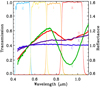 |
Fig. 1 SDSS filter transmission curve and average spectra of the Bus-DeMeo representative types. The spectra are normalized at 550 nm. |
2.2 Transformation from 2D Reflectance to 3D Colors
Traditionally for asteroid taxonomy, Principal Component Analysis has been the primary technique used to distinguish classes. Bus & Binzel (2002b) used a statistical method to determine tax-onomic classes based on the shape of the reflectance spectra, namely the spectral slope shortward of 0.75 μm and the depth of 1 μm absorption band, which are the principal components. DeMeo et al. (2009) used the principal components (slope and band depth) obtained with VIS-NIR spectra of 371 asteroids. DeMeo & Carry (2013) convert SDSS colors to their spectral analogs in the 2D color space (slope and z-i color) to classify over 34000 unique objects using the color space information of those 371 asteroids. Similarly, in this work we convert reflectance spectra of DeMeo et al. (2009) sample to SDSS colors by convolving them with the SDSS filter transmission curves (see Fig. 1). We compute the convolved flux ratio in the g band and i band to have (g-i) color, while we compute the convolved flux ratio in i and z band, to obtain (i-z) color, which are analogs of principal components defined by Bus & Binzel (2002a) and DeMeo et al. (2009).
In order to overcome the limitation set by the previous studies (artificially drawn boundaries), we introduce the griz color, a new color for asteroid taxonomy; the sum of g-r, g-i, and g-z colors represents the flux values of the normalized reflectance in the SDSS bands. We then classify 4213 MOC4 objects based on the distribution of those in the 3D color space defined with the three colors shown in Fig. 2. This newly defined color adds an extra dimension. The mathematical meaning and benefits of applying the griz color is further described in Sect. 4.1.
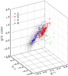 |
Fig. 2 Three-dimensional convolution color diagram of the DeMeo & Carry (2013) spectra and MOC4 dataset. Black background dots represent MOC4 photometric data without their spectral measurements. |
3 Clustering for Taxonomy Assignment
Clustering is one kind of machine learning method to identify structures in a given dataset; there are numerous methods of clustering. The exploration of the data in the 3D color space as shown in Fig. 2 informs us that the structure traced by the objects with the known taxonomy types can be well described by Gaussian shapes in the color space. As presented below, we chose Gaussian mixture models as an adequate clustering model to deduce taxonomy types. The interpretation of the inferred mixture results is not difficult and is easily understandable because of the model’s concise and robust prescription and implementation.
We applied two clustering methods using Gaussian mixtures to identify known taxonomy types in the 3D color space. The two methods have been successfully used in astronomy (Shin et al. 2009, 2012, 2018). The first method (hereafter method A) uses an infinite Gaussian mixture model to describe the distribution of objects as a mixture of multiple Gaussian distributions in multi-dimensional color space without fixing the number of the components beforehand. This method simply tries to find a concentration of data in multi-dimensional color space even though we already know the taxonomy types of some objects with measured colors. Therefore, if there are not enough data to be identified as concentrated clusters, method A fails to recover these low-density clusters. The second method (hereafter method B) is a finite Gaussian mixture model that needs to predefine the number of Gaussian mixture components, and we adopt method B as a semi-supervised machine learning method (Chapelle et al. 2010) that uses the colors of a few objects with known taxonomy types as a guide to infer the mixture properties. In method B, new types cannot be found since the number of clusters is fixed as the number of the given objects with the known taxonomy types. After estimating the mixture of Gaussian components that describe the color distribution of the input data, the two methods assign taxonomy types (i.e., cluster memberships) differently, as described later. If some objects have consistent taxonomy assignments between these multiple methods, we can consider that their derived taxonomy types are more reliable than others.
Our usage of the unsupervised and semi-supervised learning methods requires our interpretation of the clustering results in deriving the identification of the clusters in terms of the taxonomy types and evaluating the clustering quality with the comparison to the distribution of the known taxonomy types in the color space (e.g., Kiar et al. 2017).
3.1 Methods
The color distribution of the input data are described as multiple 3D Gaussian mixtures by the following equation:
![Mathematical equation: $ \matrix{ {p\left( x \right)} \hfill & { = \sum\limits_{k = 1}^K {{w_k}{1 \over {{{\left( {2\pi } \right)}^{D/2}}{{\left| {{\sum _k}} \right|}^{1/2}}}}\exp \left[ { - {1 \over 2}{{\left( {x - {\mu _{\rm{k}}}} \right)}^T}\sum\nolimits_k^{ - 1} {\left( {x - {\mu _{\rm{k}}}} \right)} } \right]} } \hfill \cr {} \hfill & { = \sum\limits_{k = 1}^K {{w_k}N\left( {x|{\lambda _{\rm{k}}},{\sum _{\rm{k}}}} \right).} } \hfill \cr } $](/articles/aa/full_html/2022/08/aa39551-20/aa39551-20-eq1.png) (1)
(1)
Here, k is an index over K mixtures, x is the vector of object colors, D is the dimension of the color space (i.e., D = 3 in this paper), and wk is a mixing fraction. The centers and covariances of the mixture components are μk and Σk, respectively. Method A assumes that the number of components is infinity by considering K as a stochastic parameter that needs to be inferred, while method B fixes K to a specific value. In our case, K is equal to 12 in method B since our data consists of 12 taxonomic types and includes known samples of the 12 types.
Our two methods estimate the parameters of the mixtures of Gaussian distributions differently. When using method A to describe the color distribution, we use the Dirichlet process in a non-parametric Bayesian inference of the parameters for the mixtures as well as a Markov chain Monte Carlo (MCMC) algorithm (Rasmussen 1999; Liverani et al. 2015; Hastie et al. 2015). Therefore, we acquire posterior distributions of the parameters such as K, wk, μk, and Σk in method A1. Method B adopts an expectation-maximization iterative algorithm to find the parameters of the mixture models for a given number of mixtures (Bishop 2006; Chen & Maitra 2015). We obtain the maximum-likelihood estimation of the parameters in method B. When method B updates the assignment of mixture components over iterations in the expectation-maximization algorithm, the objects with known taxonomy types do not change their mixture assignments, and they work as an anchor in the color distribution for evaluating wk, μk, and Σk. We present the maximum a posteriori (MAP) estimation of the parameters in method A below, and the best estimation of the parameters in method B corresponds to the maximum likelihood estimation.
We have to identify which taxonomic type matches each cluster in method A, whereas identification of taxonomy types is consequently derived from a few objects with known taxonomic types in method B. Because we already know the colors of 318 objects with 12 known taxonomy types (A, B, C, D, K, L, Q, R, S, T, V, and X), we can determine the correspondence between the mixture components and the known taxonomic types in method A.
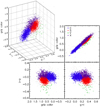 |
Fig. 3 Three-dimensional clustering diagram for MOC4 without any information of known asteroid types and colors in the method A1 taxonomy assignment with the posterior dissimilarity matrix. Different colors correspond to different taxonomy classification memberships: C type (blue), S type (red), V type (lime green), X type (purple), and Unassigned (small black). |
3.2 Results
The taxonomy assignment (i.e., cluster membership) in method A depends on a posterior dissimilarity matrix of mixture assignments derived from the MCMC samples. The optimal determination of cluster membership corresponds to the case of partitioning around medoids on the dissimilarity matrix (Liverani et al. 2015). We find six clusters in this cluster membership assignment, and we interpret four of them as C, S, V, and X types because of their color distributions and their similarity to those of known taxonomy samples shown in Fig. 3. Table 1 shows the results of this taxonomy assignment (hereafter method A1).
We also produce a different set of cluster memberships and taxonomy types incorporating the MAP estimation of the mixture parameters in method A. We present the mixture parameters wk, μk, and Σk for the resulting 13 mixture components in the MAP estimation of method A (see Table 2). This cluster membership assignment given in Table 3 is determined by finding the maximum posterior of component inclusion (i.e., membership weight)
 (2)
(2)
for each data with the estimated parameters  , and
, and  . This method results in 13 mixtures where only four clusters correspond to the meaningful taxonomy types C, S, V, and X (hereafter, method A2; see Table 3). The cluster membership in the MAP estimation is different from that derived from the dissimilarity matrix. While the MAP estimation simply works as a point estimation of the parameter values, the cluster membership assignment using the dissimilarity matrix embraces entire information in the posterior MCMC samples.
The numbers of consistent assignments between the two ways in method A are 1551, 1774, 17, and 260 for C, S, V, and X types, respectively. These numbers correspond to approximately 37%, 42%, 0.40%, and 6.2% for C, S, V, and X types, respectively, or 3602 of the total 4213 objects. We expect these objects with the consistent assignments to have more reliable taxonomy assignments than others.
Method B offers different taxonomic types with its estimation of the maximum posterior of component inclusion (i.e., membership weight). Although we consider the 12 known tax-onomic types by including their known samples, the mixtures found in method B appear to have meaningful structures corresponding to only the seven taxonomy types (C, D, K, L, S, V, and X) shown in Fig. 4 and summarized in Table 4.
Table 5 presents the taxonomic types found in method B with the normalized membership weights for the estimated 12 mixtures even though the only 7 mixtures display valid structures in the color space. If a single cluster membership weight dominates the others, the type assignment is quite reliable. For example, object 1999 NO55 has the largest and dominant cluster membership weight (0.93) for cluster 9, which corresponds to taxonomy type S (see Table 5). The taxonomic classification of object 2000 HA41 is not strongly supported by method B since its largest cluster membership weight is merely 0.31 for taxo-nomic type D. Among the 4213 objects used as input data, the number of objects with weights higher than 0.9 in the membership assignment by method B are 30, 29, 0, 23, 306, 17, and 0 for types C, D, K, L, S, V, and X, respectively. When counting the objects with a membership assignment mixture weight higher than 0.5, we recover 1093, 252, 129, 240, 1022, 57, and 235 objects forthe types C, D, K, L, S, V, and X, respectively.
The mixture parameters derived here (Tables 2 and 4) can be used to infer taxonomic types of objects for newly acquired color measurements. For example, if we suppose that for object 1999 NG53 we acquire a new measurement of color (0.28, −0.06, 0.69), which is actually what we include as the input data for clustering, the new measurement becomes a new x in Eq. (2), and we can estimate the membership weights of taxonomic types for the new color with the derived parameters  , and
, and  in either Table 2 or 4. If the new color measurement is in a sub-dimension such as g − i or i − z, we can still use the derived parameters to infer taxonomic types in terms of a marginalized distribution of the estimated Gaussian mixture distributions.
Combining the three clustering membership results given in Tables 1, 3, and 5 helps us sort out the most reliable taxonomic type assignments for the C, S, V, and X types considered in the three different results. One simple way of ensemble learning (Brown 2017) is accepting only the consistent taxonomic assignments among the three different assignments inferred by methods A and B (see Sagi & Rokach 2018; Strehl & Ghosh 2003; Ghosh & Acharya 2011, for a review). In this way we can select the objects with the most reliably inferred taxonomic types (e.g., Shin et al. 2018). Table 6 presents the objects with the C, S, V, and X taxonomic types that are in agreement among the three different inferences.
Among the 4213 objects we find 1176 (28%), 1104 (26%), 16 (0.38%), and 0 (0%) objects with the consistent taxonomic assignments for C, S, V, and X types, respectively. Focusing on objects with X type in the method A assignment, which means those that appear consistently in X-type taxonomy of method A1 and A2, D and L types correspond to 180 and 60 objects in method B assignment, respectively (see Fig. 5). K- and X-type objects in method B do not belong to the group of X-type objects inferred in the method A assignment. Since method B can cluster minor types such as D, L, and K separately from the large X-type cluster while method A cannot, there is not always agreement between methods A and B for objects assigned as X type in method A.
The lack of consistent X-type assignments between methods A and B is not a surprising result when we check taxonomy inference of the 318 Bus-DeMeo samples in method A. These samples are not used in the training of method A because method A is an unsupervised learning method. For 44, 173, 13, and 31 samples of C, S, V, and X types, respectively, in the Bus-DeMeo data we use method A2 to derive the taxonomy assignments with the derived MAP mixture parameters (i.e., Table 2). The derived taxonomy types of 42, 172, 13, and 0 objects are the same as the Bus-DeMeo taxonomy assignment for C, S, V, and X types, respectively. The color ranges of the mixture associated with X type is found to be strongly intruded by other C, S, and V types in method A (see Figs. 3 and 4). Checking consensus between methods A and B affirms that the X-type assignment in method A is not conclusive while C-, S-, and V-type assignments in method A is more reliable than the X-type assignment.
Since our method A belongs to the unsupervised learning, our result (in particular method A2) cannot be shown as a supervised learning method (e.g., Carvano et al. 2010; Erasmus et al. 2018, 2019); the result has been tested and presented with the assumption that the samples used in training are complete and distributed in the same way as the unknown test samples (see Dundar et al. 2007, for discussion). Instead, we can present the fraction of the Bus-DeMeo reference objects, which are not included in the training step of method A2, for the correct and incorrect clustering assignment in terms of the known taxonomy. As estimated from the numbers mentioned above, the fraction of correct clustering assignments, which is similar to classification accuracy in supervised learning, is about 95.5, 98.9, 100.0, and 0% for C, S, V, and X types, respectively, in method A2.
We also inspect how method A2 assigns clustering membership for the Bus-DeMeo samples in taxonomy groups not represented by method A2 (i.e., A, B, D, K, L, Q, R, and T). All B-type samples appear to be members of the C-type cluster. For the D-type samples, the dominant 9 objects among 13 samples are assigned to the X type which is mainly influenced by the C, S, and V clusters in method A2 (see Figs. 3 and 4). The single R-type object in the Bus-DeMeo samples is included in the V cluster by method A2. The S cluster includes the most objects of the other types. Therefore, the precision estimation of the correct taxonomy assignment for the C, S, V, and X become 63.6, 77.1, 92.9, and 0%, respectively. We note that these numbers cannot be interpreted as precision presented for supervised learning results.
Taxonomy types in method A with the dissimilarity matrix.
MAP parameter estimation of mixture components in method A.
Taxonomy types in method A with the MAP estimation of the parameters.
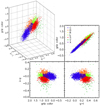 |
Fig. 4 Three-dimensional clustering diagram for MOC4 with known asteroid types and colors of DeMeo dataset in the method B taxonomy assignment. Different colors correspond to different taxonomy classification memberships: C (blue), D (orange red), K (yellow), L (lime), S (red), V (lime green), X (purple), and Unassigned (small black). |
Parameter estimation of mixture components in method B.
4 Discussion and Conclusion
4.1 New Features
In previous studies taxonomic classification of asteroids in SDSS was done in 2D parameter space using the slope (or g-i) and the absorption depth (or i-z), for instance. In this paper we introduced an additional parameter, the griz color, which is the flux value of the normalized reflectance in the SDSS bands. As is evident in Figs. 3, 4, 5, and 6, the griz color is not orthogonal to (g-i) and (i-z) in the newly defined color space. Consequently, as the slope (or g-i) grows, the area that it makes becomes larger; in the meantime, as the absorption depth (or i-z) increases it becomes smaller. This color exhibits a significantly wide distribution ranging from −1.0 to +2.0. As shown in Fig. 6, the distribution of taxonomies is different depending on which direction we look in 3D space. We note that in Fig. 6 the X and K types are both visible in the middle from the +griz direction, while only X type is seen from the −griz direction as K type is hidden from view. The same applies for −(g-i) and +(g-i), in parallel, −(i-z) and +(i-z) directions.
Likewise, most of the surface area of L type is clearly visible in the +griz direction; on the other hand, a fairly large fraction of L-cloud is obscured by S-, D-, and X-clouds. Because of the overlapping nature of the spatial distribution, we cannot completely eliminate a level of uncertainty in asteroid taxonomy, for the present. If we have a sufficient number of spectra to be used for reference points, we should be able to make a clearer division. Interactive plots are made available on the website2 where the 3D structure of the clouds can be explored. As (g-i), (i-z), and the griz colors display fairly continuous distribution, the 3D structure (the cloud of data points) that the three colors create also exhibits this property. It is naturally due to the continuously changing nature of the reflectance spectra. Remarkably, the 2D swarms revealed in various forms of principal component diagrams has proven to be the “shadow” of the 3D structure projected on the 2D “floor.”
Taxonomy types in method B.
Objects with the consistent taxonomy types in methods A and B.
4.2 Objects Without Assigned Taxonomic Types: Their True Nature
The black dots that are lying outside the color-coded (taxonomy-assigned) clusters in the relevant figures are the unassigned data points. Such objects without assigned taxonomic types (hereafter OWATs) are currently unidentifiable, and we do not know their physical nature; nevertheless, the newly adopted machine learning method is based on Bus-DeMeo taxonomy system. In order to check if the distribution of such OWATs have relevance to photometric error, we plotted the data according to error, yet we did not find any clear and systematic trend. Hence, it would be reasonable to conclude that they indeed exist, and that we need to explore and understand their true physical nature in this 3D color space.
In order to discover their true nature, we should obtain reflectance spectra of those OWATs and match their spectra with meteorite analogs for precise identifications. We expect the 3D taxonomy to evolve as we assign taxonomy to and discover the nature of these OWATs in the taxonomically and geophysically unexplored (hence unidentified) territories in the 3D color space.
4.3 Models and Training Data
We suggest multiple ways to use our clustering results with the inferred taxonomy types. First, if people want to pin down the most reliable C-, S-, V-, and X-type objects, we recommend using Table 6 to identify them. Second, when people want to identify various taxonomic types (in particular C, D, K, L, S, V, and X types) or choose objects with a certain reliability threshold, they need to use Table 5. Third, objects with highly uncertain taxonomy assignments might be interesting targets for further studies, and recognizing them requires either an inspection of the disparity between Tables 1 and 5 or an examination of the low-probability taxonomy assignments presented in Table 5.
Taxonomic types that overlap in 2D space appear to be able to be distinguished in 3D space. This is a better reflection of the parametric representation of each taxonomy and shows that it is useful for determining taxonomic classification of asteroids. However, the accuracy of the taxonomy determined by this method is not guaranteed. It is necessary to confirm the spec-troscopic observation results. Nevertheless, at the present time it is significant that the results of statistical approaches using the finite spectral samples can probably determine taxonomies of asteroids for their photometric results.
Increasing the size of the photometric training samples plays an important role in improving the clustering results of method A where the number of training samples and the density of the samples in the color space affect the quality of the clustering results. When we collect more photometric samples, we expect to unveil diverse structures in the color space including peculiar or unknown taxonomy populations, and to define color boundaries with certainty for major populations such as C, S, V, and X types. Future surveys such as the Legacy Survey of Space and Time (LSST) will produce multi-band optical data for the unprecedented large number of asteroids that can cover the diverse color populations (Jones et al. 2016).
Gathering more spectroscopically confirmed samples will also play a critical role in improving the results from our clustering methods. In particular, the added data with confirmed taxonomic types will substantially improve the reliability of the results from method B, which explicitly uses data with known taxonomic types in clustering (see Cozman et al. 2003, for discussion). We cannot find indicative structures of some taxonomic types (e.g., A, B, Q, R, and T) in method B due to an insufficient sample size of objects with already known types. The number of known taxonomy samples for these types is less than six, and method B fails to infer the cluster structure with such a small number of samples. The result of method B also demonstrates that the membership determination for the types K and X is not as confident as for other types (e.g., C, D, L, S, and V). Future spectroscopic observations such as the proposed mission CASTAway (Bowles et al. 2018) can substantially increase the number of spectroscopically confirmed taxonomy samples, covering a broad range of taxonomy types.
We expect others to use the published information on the trained models such as the cluster membership probabilities and model parameters in methods A and B with their own prior probability or model results. In particular, people may conceive of a new way to combine the results of models A and B instead of simply checking for agreement between the two models (e.g., Nguyen et al. 2020). For example, a stacking approach (Wolpert 1992) can be adopted to estimate a better method of combining our multiple results or combining our results with other taxonomy assignment results. The Bayesian estimation of a new posterior probability for taxonomy assignment is also possible in combining our model likelihood with other prior probabilities or in updating our model likelihoods. We provide simple Python scripts that can be used to infer asteroid taxonomy for given colors, our taxonomy result tables, as well as the interactive plots at our website.
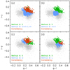 |
Fig. 5 Two-dimensional projection plots for consistent taxonomy objects. Different colors correspond to X-type assignments in method A (green; consistent objects in method A1 and A2), comparative taxonomy types in method B (blue), consistent objects between method A and B assignments (red), and all our samples (black). D- and L-type objects in method B correspond to a large portion of objects with X type in the method A result, whereas K and X types in method B do not correspond to X type in method A. |
4.4 Implications for Taxonomic Distribution of Asteroids
We plot the spatial distribution of 4213 asteroids with assigned taxonomy from method B in Fig. 7. The semi-major axis bins we chose are 0.1 AU wide ranging from 1.2 to 5.4 AU from the sun. The MOC4 objects in Hungarias (1.78−2.05 AU); the inner (2.05−2.5 AU), the middle (2.5−2.82AU), and the outer (2.82−3.27 AU) mainbelt (IMB, MMB, and OMB, respectively); Cybeles (3.27−3.7 AU); Hildas (3.7−4.2 AU); and Jupiter Trojans (JT, 5.05−5.40 AU) are included in this study. We then calculated the biased fraction of asteroids in each bin in Fig. 7a, and plot the objects in semi-major axis versus eccentricity proper orbital element plane in Fig. 7b. We note that two-thirds of the asteroids with low orbital inclinations are excluded in Fig. 7 as we applied the galactic latitude cutoff. We classified six objects outside these regions, five in the near-Earth object (NEO) and Mars Crosser (MC) regions, and 1 near ~4.6AU between the Hilda and Trojan regions. For a larger sample of NEOs and MCs in SDSS see Carry et al. (2016).
In these figures, the distribution of asteroids in Hungarias and IMB-MMB regions is dominated by S type (11%, 33% and 41% in Hungarias, IMB, and MMB, respectively) out to 3 AU, while C type takes the position in OMB (45.6%) and beyond. The apparent lack of X-type asteroids in the Hungaria family is due to the exclusion of low orbital inclination objects as we applied a more stringent galactic latitude cutoff. While X-type asteroids occupy a large fraction of Hungarias (17.7%), the fraction drops in the IMB (7.3%) and MMB (6.8%) sections to suddenly increase (~30%) in the inner OMB. X type is known to be composed of three subtypes, E, M, and P (Tholen 1984), where P types show the lowest albedo with a featureless reddish spectra. They are found mostly in OMB and beyond (Lazzarin et al. 1995) with an apparent peak at 4 AU (McSween 1999). Nevertheless, we find the peaks of X and P types to be located at 3-3.2 AU in Fig. 7 of this work and Fig. 11 of DeMeo & Carry (2013), although a one-to-one comparison is difficult as we do not separate E, M, and P types in this study.
At the same time, the V-type fraction grows in the IMB where the Vesta family dominates, while it becomes almost negligible in OMB. We then calculated the observed fraction of some minor taxonomy types such as D, K, and L across the main belt. The portion of D type in the outer OMB is between 10% and 20% (e.g., from one-fourth to one-eighth of the C-type fraction in this section); the fraction dramatically increases among Hilda (62.5%) and peaks at JT swarms (72.2%) to become an absolute majority. However, it is significant that D-type asteroids are also discovered in the innermost asteroid zone such as Hungarias (5.4%) and IMB (5.1%) (see DeMeo & Carry 2013; DeMeo et al. 2014). On the other hand, both K and L types are relatively evenly distributed in Hungarias and across the mainbelt, even if their contribution is not very significant. The observed L-type fraction is ~10% throughout the 2.2-2.7 AU region, while the K-type fraction demonstrates two less prominent peaks at 2.0 and 3.0 AU in our binning scheme. Due to the relatively small number of the sample (4123), hence sparsely populated data points in the orbital parameter plane, study of the dynamical structure of the asteroid belt is rather difficult. If we expand the sample with either better photometric qualities or spectroscopic measurements, a higher resolution picture of the dynamical families should be revealed (Ivezić et al. 2002; Parker et al. 2008).
Our results are generally consistent with those found in DeMeo & Carry (2013) for the biased results shown in their Fig. 10 and with other earlier works (Bus & Binzel 2002a; Mothé-Diniz et al. 2003). For example, S-types dominate the IMB and MMB by number, and the switch to C types being more populous occurs in the OMB. Discrepancies between our work and previous studies are attributable to more low-inclination objects being excluded from this work due to our more stringent data quality cutoff including galactic latitude constraints and to the small sample sizes among Hildas and Jupiter Trojans. These discrepancies include a smaller contribution of V types (Vesta family) in the IMB and K types (Eos family) in the OMB, and different relative fractions of X and D in the Hildas and Jupiter Trojans. A larger sample size for Hildas and Trojans than is available for SDSS has been studied by NEOWISE (Grav et al. 2012a,b).
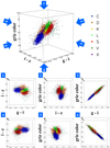 |
Fig. 6 Perspective view of the 3D clustering results in method B. The color-coding is the same as in Fig. 4. Different colors correspond to different taxonomy classification memberships for C (blue), D (orange red), K (yellow), L (lime), S (red), V (lime green), X (purple), and unassigned (black). The overlapping members of each type in the 2D plane seem to be separated by relatively clear boundaries in 3D space. |
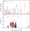 |
Fig. 7 Spatial distribution of 4213 SDSS MOC4 asteriods. (a) Biased fraction of each type in each 0.1 AU bin. (b) Taxonomy distribution of asteroids in proper orbital elements plane (semi-major axis vs. orbital eccentricity). |
4.5 The Future of Asteroid Taxonomy
In this work, we put forth a method for the taxonomic classification of asteroids based on the clustering analysis of the photometric data. This classification scheme can also be simply represented by a triplet or multiplet of photometric colors, either in LSST or in Johnson-Cousins photometric systems. Applying our methods with observation data acquired in these bands may allow taxonomic identification of interesting populations. Colors in these different bands may help us identify minor taxonomy groups that are not strongly concentrated in the SDSS dataset.
Including NIR colors in clustering analysis will be one way of extending our methodology to cover NIR taxonomy classification. Popescu et al. (2018) presented possible taxonomy classification in the J − Ks and Y − J color-color space by adopting straight line boundaries among the types. We plan to investigate the optical-NIR combined clustering analysis of the objects studied in this paper, generating the Gaussian mixture models in color space over the optical-NIR colors and comparing the results from the current analysis and the combined analysis.
Our taxonomy method is extensible for many asteroid studies. We can combine the study of space weathering trends in S-complex subtypes with their color distribution of 3D parameter space. Furthermore, we are cautiously optimistic that the taxonomic distributions of asteroid families in proper orbital element space may reveal a more detailed interpretation of their origin and evolution.
Acknowledgements
This study is supported by Korea Astronomy and Space Science Institute. FED acknowledges funding from the National Aeronautics and Space Administration under Grant nos. 80NSSC18K0849 and 80NSSC18K1004 issued through the Planetary Astronomy Program. We would like to thank anonymous reviewer for his/her careful reading of our manuscript and insightful comments with valuable suggestions.
References
- Bishop, C. M. 2006, Pattern Recognition and Machine Learning (Information Science and Statistics) (Secaucus, NJ, USA: Springer-Verlag New York, Inc.) [Google Scholar]
- Bowles, N. E., Snodgrass, C., Gibbings, A., et al. 2018, Adv. Space Res., 62, 1998 [NASA ADS] [CrossRef] [Google Scholar]
- Brown, G. 2017, Ensemble Learning, eds. C. Sammut, & G. I. Webb (Boston, MA: Springer US), 393 [Google Scholar]
- Bus, S. J., & Binzel, R. P. 2002a, Icarus, 158, 146 [Google Scholar]
- Bus, S. J., & Binzel, R. P. 2002b, Icarus, 158, 106 [CrossRef] [Google Scholar]
- Carry, B., Solano, E., Eggl, S., & DeMeo, F. E. 2016, Icarus, 268, 340 [CrossRef] [Google Scholar]
- Carvano, J. M., Hasselmann, P. H., Lazzaro, D., & Mothé-Diniz, T. 2010, A&A, 510, A43 [NASA ADS] [CrossRef] [EDP Sciences] [Google Scholar]
- Chapelle, O., Schlkopf, B., & Zien, A. 2010, Semi-Supervised Learning, 1st edn. (The MIT Press) [Google Scholar]
- Chapman, C. R., Johnson, T. V., & McCord, T. B. 1971, A Review of Spectrophotometric Studies of Asteroids, ed. T. Gehrels, 267, 51 [Google Scholar]
- Chapman, C. R., Morrison, D., & Zellner, B. 1975, Icarus, 25, 104 [NASA ADS] [CrossRef] [Google Scholar]
- Chen, W.-C., & Maitra, R. 2015, EMCluster: EM Algorithm for Model-Based Clustering of Finite Mixture Gaussian Distribution, R Package, URL http://cran.r-project.org/package=EMCluster [Google Scholar]
- Cozman, F. G., Cohen, I., & Cirelo, M. C. 2003, in Proceedings of the Twentieth International Conference on International Conference on Machine Learning, ICML’03 (AAAI Press), 99 [Google Scholar]
- DeMeo, F. E., & Carry, B. 2013, Icarus, 226, 723 [NASA ADS] [CrossRef] [Google Scholar]
- DeMeo, F. E., Binzel, R. P., Slivan, S. M., & Bus, S. J. 2009, Icarus, 202, 160 [Google Scholar]
- DeMeo, F. E., Binzel, R. P., Carry, B., Polishook, D., & Moskovitz, N. A. 2014, Icarus, 229, 392 [NASA ADS] [CrossRef] [Google Scholar]
- Dundar, M., Krishnapuram, B., Bi, J., & Rao, R. B. 2007, in Proceedings of the 20th International Joint Conference on Artifical Intelligence, IJCAI’07 (San Francisco, CA, USA: Morgan Kaufmann Publishers Inc.), 756 [Google Scholar]
- Erasmus, N., McNeill, A., Mommert, M., et al. 2018, ApJS, 237, 19 [NASA ADS] [CrossRef] [Google Scholar]
- Erasmus, N., McNeill, A., Mommert, M., et al. 2019, ApJS, 242, 15 [NASA ADS] [CrossRef] [Google Scholar]
- Ghosh, J., & Acharya, A. 2011, WIREs Data Mining and Knowledge Discovery, 1, 305 [CrossRef] [Google Scholar]
- Grav, T., Mainzer, A. K., Bauer, J., et al. 2012a, ApJ, 744, 197 [NASA ADS] [CrossRef] [Google Scholar]
- Grav, T., Mainzer, A. K., Bauer, J. M., Masiero, J. R., & Nugent, C. R. 2012b, ApJ, 759, 49 [NASA ADS] [CrossRef] [Google Scholar]
- Hasselmann, P. H., Fulchignoni, M., Carvano, J. M., Lazzaro, D., & Barucci, M. A. 2015, A&A, 577, A147 [NASA ADS] [CrossRef] [EDP Sciences] [Google Scholar]
- Hastie, D. I., Liverani, S., & Richardson, S. 2015, Stat. Comput., 25, 1023 [CrossRef] [Google Scholar]
- Ivezić, Ž., Tabachnik, S., Rafikov, R., et al. 2001, AJ, 122, 2749 [Google Scholar]
- Ivezić, Ž., Lupton, R. H., Juric, M., et al. 2002, AJ, 124, 2943 [CrossRef] [Google Scholar]
- Jones, R. L., Juric, M., & Ivezic, Ž. 2016, in IAU Symposium, 318, Asteroids: New Observations, New Models, eds. S. R. Chesley, A. Morbidelli, R. Jedicke, & D. Farnocchia, 282 [Google Scholar]
- Kiar, A. K., Barmby, P., & Hidalgo, A. 2017, MNRAS, 472, 1074 [CrossRef] [Google Scholar]
- Kitamura, M. 1959, PASJ, 11, 79 [Google Scholar]
- Lazzarin, M., Barbieri, C., & Barucci, M. A. 1995, AJ, 110, 3058 [NASA ADS] [CrossRef] [Google Scholar]
- Lazzaro, D., Angeli, C. A., Carvano, J. M., et al. 2004, Icarus, 172, 179 [NASA ADS] [CrossRef] [Google Scholar]
- Liverani, S., Hastie, D., Azizi, L., Papathomas, M., & Richardson, S. 2015, J. Stat. Softw., 64, 1 [CrossRef] [Google Scholar]
- Mainzer, A., Bauer, J., Grav, T., et al. 2011, ApJ, 731, 53 [Google Scholar]
- Masiero, J. R., Mainzer, A. K., Grav, T., et al. 2011, ApJ, 741, 68 [Google Scholar]
- McSween, Harry Y. J. 1999, Meteorites and their Parent Planets [Google Scholar]
- Mothé-Diniz, T., Carvano, J. M. Á., & Lazzaro, D. 2003, Icarus, 162, 10 [CrossRef] [Google Scholar]
- Nguyen, T. T., Luong, A. V., Dang, M. T., Liew, A. W.-C., & McCall, J. 2020, Pattern Recogn., 100, 107104 [NASA ADS] [CrossRef] [Google Scholar]
- Parker, A., Ivezicć, Ž., Juricć, M., et al. 2008, Icarus, 198, 138 [NASA ADS] [CrossRef] [Google Scholar]
- Popescu, M., Licandro, J., Carvano, J. M., et al. 2018, A&A, 617, A12 [NASA ADS] [CrossRef] [EDP Sciences] [Google Scholar]
- Rasmussen, C. E. 1999, in Proceedings of the 12th International Conference on Neural Information Processing Systems, NIPS’99 (Cambridge, MA, USA: MIT Press), 554 [Google Scholar]
- Sagi, O., & Rokach, L. 2018, WIREs Data Mining Knowledge Discov., 8, e1249 [CrossRef] [Google Scholar]
- Shin, M.-S., Sekora, M., & Byun, Y.-I. 2009, MNRAS, 400, 1897 [NASA ADS] [CrossRef] [Google Scholar]
- Shin, M.-S., Yi, H., Kim, D.-W., Chang, S.-W., & Byun, Y.-I. 2012, AJ, 143, 65 [NASA ADS] [CrossRef] [Google Scholar]
- Shin, M.-S., Chang, S.-W., Yi, H., et al. 2018, AJ, 156, 201 [NASA ADS] [CrossRef] [Google Scholar]
- Strehl, A., & Ghosh, J. 2003, J. Mach. Learn. Res., 3, 583 [Google Scholar]
- Tedesco, E. F., Williams, J. G., Matson, D. L., et al. 1989, AJ, 97, 580 [NASA ADS] [CrossRef] [Google Scholar]
- Tholen, D. J. 1984, PhD thesis, University of Arizona, Tucson, USA [Google Scholar]
- Wolpert, D. H. 1992, Neural Netw., 5, 241 [CrossRef] [Google Scholar]
- Zellner, B. 1973, in BAAS, 5, 388 [NASA ADS] [Google Scholar]
- Zellner, B., Tholen, D. J., & Tedesco, E. F. 1985, Icarus, 61, 355 [NASA ADS] [CrossRef] [Google Scholar]
We adopt a hyperparameter α = 2:2 by checking the clustering results and their correspondence to the colors of the known taxonomy types (see Shin et al. 2009, for discussion).
All Tables
All Figures
|
Fig. 1 SDSS filter transmission curve and average spectra of the Bus-DeMeo representative types. The spectra are normalized at 550 nm. |
| In the text | |
|
Fig. 2 Three-dimensional convolution color diagram of the DeMeo & Carry (2013) spectra and MOC4 dataset. Black background dots represent MOC4 photometric data without their spectral measurements. |
| In the text | |
|
Fig. 3 Three-dimensional clustering diagram for MOC4 without any information of known asteroid types and colors in the method A1 taxonomy assignment with the posterior dissimilarity matrix. Different colors correspond to different taxonomy classification memberships: C type (blue), S type (red), V type (lime green), X type (purple), and Unassigned (small black). |
| In the text | |
|
Fig. 4 Three-dimensional clustering diagram for MOC4 with known asteroid types and colors of DeMeo dataset in the method B taxonomy assignment. Different colors correspond to different taxonomy classification memberships: C (blue), D (orange red), K (yellow), L (lime), S (red), V (lime green), X (purple), and Unassigned (small black). |
| In the text | |
|
Fig. 5 Two-dimensional projection plots for consistent taxonomy objects. Different colors correspond to X-type assignments in method A (green; consistent objects in method A1 and A2), comparative taxonomy types in method B (blue), consistent objects between method A and B assignments (red), and all our samples (black). D- and L-type objects in method B correspond to a large portion of objects with X type in the method A result, whereas K and X types in method B do not correspond to X type in method A. |
| In the text | |
|
Fig. 6 Perspective view of the 3D clustering results in method B. The color-coding is the same as in Fig. 4. Different colors correspond to different taxonomy classification memberships for C (blue), D (orange red), K (yellow), L (lime), S (red), V (lime green), X (purple), and unassigned (black). The overlapping members of each type in the 2D plane seem to be separated by relatively clear boundaries in 3D space. |
| In the text | |
|
Fig. 7 Spatial distribution of 4213 SDSS MOC4 asteriods. (a) Biased fraction of each type in each 0.1 AU bin. (b) Taxonomy distribution of asteroids in proper orbital elements plane (semi-major axis vs. orbital eccentricity). |
| In the text | |
Current usage metrics show cumulative count of Article Views (full-text article views including HTML views, PDF and ePub downloads, according to the available data) and Abstracts Views on Vision4Press platform.
Data correspond to usage on the plateform after 2015. The current usage metrics is available 48-96 hours after online publication and is updated daily on week days.
Initial download of the metrics may take a while.