© R. G. Visser and M. G. Brouwers 2022

1 Introduction

Across a wide range of astrophysical scales, from asteroids to stars and beyond, many kinds of objects tend to form via the gravitational collapse of larger structures. The rotation of these objects, which tends to manifest as increased velocities when their moments of inertia decrease, is a key tool for investigating the physics of their formation. When inferring rotational trends from observations, it is often difficult to disentangle the system’s rotation at birth from its later dynamical evolution. In some cases, however, systems with largely primordial rotational distributions still contain important historical clues about the processes by which they formed.

At the smallest scale of relevance here, asteroids and comets are long since thought to form in gravitational collapses within proto-planetary disks (see e.g., Goldreich & Ward 1973; Youdin & Shu 2002; Morbidelli et al. 2009), via a small-scale mechanism now known as the streaming instability (Youdin & Goodman 2005; Johansen et al. 2007, 2009; Simon et al. 2016; Schäfer et al. 2017). Whether traces of their primordial spins remain depends chiefly on the class and size of the asteroids that are studied. At the lower end of the size distribution, smaller asteroids have a largely isotropic spin distribution, with traces of their prior rotation wiped out by intense collisional processing (see e.g., Davis et al. 1989; Bottke et al. 2005a,b; Pan & Sari 2005; Fraser 2009) or by radiation induced changes in spin such as the YORP effect, (Pravec et al. 2008; Medeiros et al. 2018; Rubincam 2000). Similarly, the largest bodies, such as Ceres and Vesta, may have accreted most of their prograde spin during later stages by pebble accretion (Johansen & Lacerda 2010; Visser et al. 2020). In between, however, an intermediate class of asteroids with diameters between ~ 100 and 500 km likely still contains key information about their rotation at birth (Steinberg & Sari 2015). Within the Solar System, the most dynamically pristine subset of these objects belong to the group of “cold classicals” that reside in the Kuiper belt. Besides being characterized by low inclinations and eccentricities, this group contains a high fraction of binary pairs (Noll et al. 2008; Fraser et al. 2017; Grundy et al. 2019) which often have strong color correlations (Benecchi et al. 2009, 2011; Marsset et al. 2020), reinforcing the idea that they formed in a single gravitational collapse – rather than by later capture. Interestingly, many of the binaries are found to have mass ratios near unity – which means that the collections of particles, or “clouds”, from which they formed must have contained substantial amounts of rotational angular momentum (Nesvorný et al. 2010; Robinson et al. 2020). Their binary orbits are not distributed isotropically and express a preferential (prograde) alignment with their center-of-mass orbit around the Sun (Grundy et al. 2019). Recently, hydrodynamic simulations have shown that such a distribution can indeed arise as the result of streaming instabilities (Nesvorný et al. 2019, 2021), but the underlying physical origin of the strong spin-orbit alignment remains poorly understood.

The trend of spin-orbit alignment continues at the scale above asteroids, where all the planets in the Solar System except Venus and Uranus rotate in the prograde direction. Theoretically, the prograde rotation of gas giants is readily explained in the context of core accretion by the torque during runaway gas accretion (Machida et al. 2008; Dittmann 2021), but systematic explanations of terrestrial spin have proven more problematic (Lissauer & Safronov 1991). Planetesimal accretion is found to deliver insufficient rotation to the accreting planet (Lissauer & Kary 1991; Dones & Tremaine 1993a), and later giant impacts fail to produce an anisotropic distribution (Safronov 1966; Dones & Tremaine 1993b). Pebble accretion could potentially provide a large, systematically prograde spin to planets (Johansen & Lacerda 2010; Visser et al. 2020), although this remains to be validated for accretion onto proto-planets with substantial envelopes, where pebbles face intense drag and sublimation (Alibert 2017; Brouwers et al. 2021; Johansen & Nordlund 2020).

In the alternative theories to core accretion, planetary rotation again finds its origin in gravitational collapse. Terrestrial cores have been proposed to form out of dense pebble traps at the edges of dead zones in the inside-out mechanism (Chatterjee & Tan 2014; Hu et al. 2016, 2018; Mohanty et al. 2018; Cai et al. 2022), whereas gas giants can form directly from gravitational instabilities of cold gas (see e.g., Kuiper 1951; Cameron 1978; Boss 1998, 2021). The obliquities of these larger planets on wide orbits are just beginning to be measured. Observations of 2M0122b seem to tentatively indicate a large obliquity (Bryan et al. 2020, 2021), while HD 106906 b more certainly spins on its side (Bryan et al. 2021). Recent smoothed-particle-hydrodynamics (SPH) and hydrodynamic simulations show that gravitational cloud collapse in gravito-turbulent disks can yield obliquities of up to 90 degrees (Jennings & Chiang 2021), although most objects seem to form with more alignment (Hall et al. 2017). For now, more observations beyond the two known cases are required to resolve the statistical spin distribution of this class of planets.

Most stars form in clusters via the collapse of dense substructures within molecular clouds, which often fragment into several thousand stars per cluster (see e.g., McKee & Ostriker 2007; Lee et al. 2012; Lee & Hennebelle 2016b). The mutual alignment of stars in these clusters has been studied in a limited context, with differing results. In the first spectroscopic studies of the young, low-mass open clusters Pleiades and Alpha Per, no spin alignment was found in the population of G, K-, or M-type stars (Jackson & Jeffries 2010; Jackson et al. 2018). This seems consistent with the older idea that stellar spins depend intimately on the local turbulence (see e.g., Fleck & Clark 1981; Belloche 2013), which itself is ultimately induced by differential galactic rotation (Renaud et al. 2013; Rey-Raposo et al. 2015; Rey-Raposo & Read 2018). Recently, however, astro-seismological measurements of red giants in the higher-mass clusters NGC 6791 and NGC 6819 were found to exhibit a strong inter-cluster spin alignment (Corsaro et al. 2017). Highresolution simulations indicate that such a spin-alignment can arise for stars above 0.7 M_⊙ when their natal star-forming clump contains more than 50% of its kinetic energy in rotation (Lee & Hennebelle 2016a; Corsaro et al. 2017). Although this rotational support might be rare (Caselli et al. 2002; Pirogov et al. 2003), mutual stellar spin alignment in such cases points to a spin-orbit alignment within the cluster, similar to the prograde rotation of asteroids and planets around a central star. Finally, we add that in the well-studied galaxies M 33 and M 51, the larger molecular clouds that host the star-forming clumps also seem to possess structural prograde rotation around the galaxy itself (Braine et al. 2018, 2020).

The preceding overview reveals a universal trend: objects that form via a gravitational collapse in the presence of an external gravitational field tend to exhibit a preferential alignment between their spins and orbital motions. Remarkably, the fact that such a spin-orbit alignment exists across different scales has received little scientific attention, and no satisfactory common explanation has yet been suggested. Perhaps the most relevant contribution to the topic is that of Mestel (1966), who considered the instantaneous condensation of patches from a differentially rotating disk (Ω(r) ∝ rⁿ). His work showed that any closed, two-dimensional patch of a disk with an increasing rotation curve (n ≥ −1) always contains prograde spin about its center-of-mass, whereas patches from a Keplerian disk (n = −3/2) can yield spin in either direction, depending on their shape. However, in many cases, the collapse will not proceed from a fully ordered state. If the relevant clouds are formed by a process in which turbulent motions play an important role, the initial rotational setup of the collapsing cloud will be much more randomized, making it unclear from the potential alone what the spin direction will be. In addition, Shmidt (1957) realized that the center-of-mass of a patch – and therefore its orbital angular momentum – could evolve during its collapse and that the final rotational direction would formally be set by the conservation of total angular momentum and energy. In his work, prograde rotation was interpreted as the result of a collapse with sufficient thermal energy loss. These calculations were later extended by Safronov (1962, 1972) but ultimately proved inconclusive due to the problem of unknown thermal losses.

In this work, we provide a different, geometrically motivated approach to the rotational evolution of collapsing clouds in orbit around an external potential, most similar to the tidal torque theory that seeks to explain galactic spins (Hoyle 1951; Peebles 1969). We show that because particles that orbit in any nonrigid cloud shear away from one another over time – and do so on curved paths – their combined center-of-mass moves toward the source of the external potential during a gravitational collapse. The orbital angular momentum that is thus liberated, adds a prograde component to the spin of the object that forms. This mechanism of prograde spin-up is most effective when the clouds are low in density prior to their collapse and when individual particles are on circular orbits, although the effect persists across a wide range of setups. Due to its universal applicability, we suggest that prograde spin-up during a gravitational collapse contributes to the ubiquity of spin-orbit alignment on different scales.

The structure of the paper is organized as follows. We begin in Sect. 2 with an illustrative analytical calculation of prograde spin-up with two-dimensional, circular orbits around a point source. In Sect. 3, we numerically verify the main analytical trends by including self-gravity and present a more visual analysis by showing the spin-up of a cloud without any initial rotation. We apply the mechanism of prograde spin-up to the formation of binary asteroids/comets via streaming instability in Sect. 4. Finally, we discuss the broader implications of our findings in Sect. 5 and conclude in Sect. 6.

2 Analytical Evaluation of Prograde Spin-up

In this section, we perform a calculation without self-gravity to illustrate how shear can transfer orbital angular momentum to rotation based on the orbital geometry. The idea behind this calculation is that objects form at the centers-of-mass of collapsing clouds, which orbit in the potential of larger objects or structures. While the nonlinear nature of a cloud collapse in the presence of an external potential is generally unsuitable for analytical modeling, the main trends can be elucidated by following cloud particles without treating self-gravity, at least while the collapse is not yet in full swing. The setup of this analytical calculation is sketched in Fig. 1. We consider a two-dimensional cloud with a uniform density σ_cl that integrates to a total mass M_cl. The particles in the cloud move around a stationary central mass M_C ≫ M_cl on circular orbits with angular velocity $\Omega =\sqrt{G{M}_C/r^3}$ at distance r. We conveniently let the initial shape of the cloud be that of a partial annulus, bounded by inner and outer circles at r₀ ± R_cl and angles ±θ₀, with R_cl = θ₀r₀, such that the cloud consists of radially separated differential arcs with length l_arc(r) = 2R_clr/r₀.

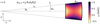Fig. 1 Schematic setup of our analytical calculation (Sect. 2). We consider a two-dimensional cloud of mass Mcl in a stationary frame, whose origin lies on the central mass MC ≫ Mcl (where the dotted lines cross). The initial shape of the cloud is that of a partial annulus, bounded by inner and outer circles with radii r0 ± Rcl and radial lines at angles ±θ0. We follow the position $\left({\overline{x}}_{\text{cl}},{\overline{y}}_{\text{cl}}\right)$ and velocity $\left({\overline{\upsilon }}_{\text{x,cl}},{\overline{\upsilon }}_{\text{y,cl}}\right)$ of the cloud’s center-of-mass over time and calculate the specific rotational angular momentum of cloud particles $\left(\widehat{z}\right)$ relative to this point as $l_{\text{rot}}=\left(x{\upsilon }_{\text{y}}-y{\upsilon }_{\text{x}}\right)-\left({\overline{x}}_{\text{cl}}{\overline{\upsilon }}_{\text{y,cl}}-{\overline{y}}_{\text{cl}}{\overline{\upsilon }}_{\text{x,cl}}\right)$, shown in the color plot at t = 0. The initial velocities of the cloud particles correspond to circular, Keplerian motion. Particles that start on the x-axis initially contribute retrograde rotation due to shear, whereas particles on the y-axis contribute prograde rotation due to curvature. The integrated result is a net initial prograde rotational angular momentum that increases over time if the cloud orbits freely (see Eq. (14b)).

2.1 Position and Velocity of Shearing Radial Arcs

First, we calculate the positions and velocities of the different radial arcs. Their angular velocities vary slightly depending on theirradial separation, causing deviations between arcs thatgrow over time. In a stationary frame, the upper (θ₊) and lower (θ₋) bounding angles of an arc are given by: $${\theta }_{\pm }=\pm {\theta }_0+{\Omega }_0{\left(\frac{r}{r_0}\right)}^{-\frac{3}{2}}t,$$(1)

where t is time after initiation. The center-of-mass of an arc can be calculated in Cartesian coordinates with their origin on M_C $\left({\overline{x}}_{\text{arc}},{\overline{y}}_{\text{arc}}\right)$ to lie at: $${\overline{x}}_{\text{arc}}=\frac{1}{2{\theta }_0}{\displaystyle {\int }_{{\theta }_{-}}^{{\theta }_0}r\cos \left({\theta }^{\prime }\right)\text{d}{\theta }^{\prime }},$$(2a) $$=\frac{r\sin \left({\theta }_0\right)\cos \left[{\Omega }_0{\left(\frac{r}{r_0}\right)}^{-\frac{3}{2}}t\right]}{{\theta }_0},$$(2b) $${\overline{y}}_{\text{arc}}=\frac{1}{2{\theta }_0}{\displaystyle {\int }_{{\theta }_{-}}^{{\theta }_0}r\sin \left({\theta }^{\prime }\right)\text{d}{\theta }^{\prime }}$$(3a) $$=\frac{r\sin \left({\theta }_0\right)\sin \left[{\Omega }_0{\left(\frac{r}{r_0}\right)}^{-\frac{3}{2}}t\right]}{{\theta }_0}.$$(3b)

As expected, it is initially located on the x-axis and subsequently orbits in a circular motion as a function of time. Trivially, its velocity components follow from the time derivatives as: $${\overline{\upsilon }}_{\text{x,arc}}=-{\Omega }_0{\left(\frac{r}{r_0}\right)}^{-\frac{3}{2}}{\overline{y}}_{\text{arc}}={\overline{\upsilon }}_{\text{y,arc}}={\Omega }_0{\left(\frac{r}{r_0}\right)}^{-\frac{3}{2}}{\overline{x}}_{\text{arc}}.$$(4)

2.2 Trajectory of the Cloud’S Center-of-mass

The calculation becomes interesting when we combine the positions of different arcs to find the center-of-mass of the whole cloud. We first note that without self-gravity, its area, being the integral over the differential arcs, remains constant over time and follows from subtracting the two partial disk areas as A_cl = 4 R_clr₀θ₀ = 4 $R_{\text{cl}}^2$. The position $\left({\overline{x}}_{\text{cl}},{\overline{y}}_{\text{cl}}\right)$ and velocity $\left({\overline{\upsilon }}_{\text{x,cl}},{\overline{\upsilon }}_{\text{y,cl}}\right)$ of the cloud’s center-of-mass can be found by radially integrating over Eqs. (2b), (3b), and (4), which yields: $$\begin{array}{c}{\overline{x}}_{\text{cl}}\left(t\right)=\frac{1}{A_{\text{cl}}}{\displaystyle {\int }_{r_0-R_{\text{cl}}}^{r_0+R_{\text{cl}}}{\overline{x}}_{\text{arc}}\left(r\right)l_{\text{arc}}}\left(r\right)\text{d}r\\ \simeq r_0\cos \left({\Omega }_{0}t\right)\end{array}$$(5a) $$+\frac{R_{\text{cl}}^2}{24r_0}\left[\left(4-9{\Omega }_0^2{t}^2\right)\cos \left({\Omega }_{0}t\right)+9{\Omega }_{0}t\sin \left({\Omega }_{0}t\right)\right],$$(5b) $$\begin{array}{c}{\overline{y}}_{\text{cl}}\left(t\right)=\frac{1}{A_{\text{cl}}}{\displaystyle {\int }_{r_0-R_{\text{cl}}}^{r_0+R_{\text{cl}}}{\overline{y}}_{\text{arc}}\left(r\right)l_{\text{arc}}\left(r\right)\text{d}r}\\ \simeq r_0\sin \left({\Omega }_{0}t\right)\end{array}$$(6a) $$+\frac{R_{\text{cl}}^2}{24r_0}\left[\left(4-9{\Omega }_0^2{t}^2\right)\sin \left({\Omega }_{0}t\right)-9{\Omega }_{0}tos\left({\Omega }_{0}t\right)\right],$$(6b)

with the corresponding velocities given by the time derivatives: $$\begin{array}{c}{\overline{\upsilon }}_{\text{x,cl}}\left(t\right)\simeq -{\Omega }_0{r}_0\sin \left({\Omega }_{0}t\right)\\ +\frac{{\Omega }_0{R}_{\text{cl}}^2}{24r_0}\left[\left(5+9{\Omega }_0^2{t}^2\right)\sin \left({\Omega }_{0}t\right)-9{\Omega }_{0}t\cos \left({\Omega }_{0}t\right)\right],\end{array}$$(7a) $$\begin{array}{c}{\overline{\upsilon }}_{\text{y,cl}}\left(t\right)=\simeq -{\Omega }_0{r}_0\cos \left({\Omega }_{0}t\right)\\ +\frac{{\Omega }_0{R}_{\text{cl}}^2}{24r_0}\left[-\left(5+9{\Omega }_0^2{t}^2\right)\cos \left({\Omega }_{0}t\right)-9{\Omega }_{0}t\sin \left({\Omega }_{0}t\right)\right].\end{array}$$(8a)

These integrals are calculated with Mathematica 12.0 and each have exact solutions in the form of long sums. We provide the Maclaurin series with the variable θ₀ ≪ 1 in order to maintain some brevity. To zeroth order, the center-of-mass follows a simple circular motion at distance r₀ from the central mass. The strongest deviation is a second-order term that includes a small initial off-set from r₀ as well as a time-dependent factor. From Eqs. (5b) and (6b), we can calculate how the distance of the cloud’s center-of-mass (r̄_cl) evolves over time: $$\delta {\overline{r}}_{\text{cl}}\left(t\right)\sqrt{{\overline{x}}_{\text{cl}}^2\left(t\right)+{\overline{y}}_{\text{cl}}^2\left(t\right)}-\sqrt{{\overline{x}}_{\text{cl}}^2\left(t=0\right)+{\overline{y}}_{\text{cl}}^2\left(t=0\right)}$$(9a) $$=-\frac{3R_{\text{cl}}^2{\Omega }_0^2{t}^2}{8r_0}.$$(9b)

Interestingly, we find that the center-of-mass in this setup moves inward with a quadratic time dependence. We show the geometrical origin of this change in Fig. 2 where we sketch the position of a cloud of particles in Keplerian motion. As the cloud shears out and angular differences increase, its shape deforms from a partial annulus into an increasingly extended single arc. Due to the curvature inherent to circular motion, the center-of-mass of this arc shifts toward the star as a function of time. If the system is evolved for a sufficiently long period of time, the center-of-mass ultimately coincides with the position of the central mass. We can further investigate the trajectory of the cloud’s center-of-mass by calculating its semimajor axis (ā_cl), which follows from the energy balance as: $${\overline{a}}_{\text{cl}}\left(t\right)=\frac{{\Omega }_0^2{r}_0^3}{2}{\left(\frac{{\Omega }_0^2{r}_0^3}{{\overline{r}}_{\text{cl}}\left(t\right)}-\frac{{\overline{\upsilon }}_{\text{y,cl}}^2\left(t\right)}{2}\right)}^{-1}.$$(10)

Again, we are mainly interested in its evolution from the initial value as a function of time, so we compute this difference (δā_cl): $$\delta {\overline{a}}_{\text{cl}}\left(t\right)={\overline{a}}_{\text{cl}}\left(t\right)-{\overline{a}}_{\text{cl}}\left(t=0\right)$$(11a) $$=-\frac{3R_{\text{cl}}^2{\Omega }_0^2{t}^2}{2r_0}.$$(11b)

In this example calculation, the semimajor axis of the cloud’s center-of-mass decreases faster than its distance to the central mass and, hence, its eccentricity increases over time. We have verified that the form of Eq. (11b) is unchanged when the shape of the cloud is altered. For example, the pre-factor of 3/2 becomes 1/8 for a cloud in the shape of a closed disk, remains 3/2 for a radial line and tends to zero for a tangential line, whose particles do not experience shear.

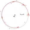Fig. 2 Illustration of the inward center-of-mass shift in our analytical example. The particles follow circular orbits around a central mass without mutual interactions. As the particles shear out over time, the ensemble deforms into an increasingly extended single arc, shifting the center-of-mass position (open circular dot) closer to the orbital midpoint.

2.3 Transfer of Orbital Angular Momentum to Rotation

If an object forms at the center-of-mass of a cloud, its shrinking semimajor axis and increasing eccentricity during the collapse reduce its orbital angular momentum $\left({\overline{L}}_{\text{cl}}\right)$, which points in the $\widehat{z}$-direction in this two-dimensional example: $${\overline{L}}_{\text{cl}}\left(t\right)=M_{\text{cl}}\left[{\overline{x}}_{\text{cl}}\left(t\right){\overline{\upsilon }}_{\text{y,cl}}\left(t\right)-{\overline{y}}_{\text{cl}}\left(t\right){\overline{\upsilon }}_{\text{x,cl}}\left(t\right)\right]$$(12a) $$\simeq M_{\text{cl}}{\Omega }_0{r}_0^2\left[1-\frac{1}{24}{\left(\frac{R_{\text{cl}}}{r_0}\right)}^2\left(1+18{\Omega }_0^2{t}^2\right)\right].$$(12b)

While the orbital angular momentum associated with the center-of-mass orbit declines, the total angular momentum of the cloud (L_tot,cl) remains constant over time, equal to: $$L_{\text{tot,cl}}={\displaystyle {\int }_{r_0-R_{\text{cl}}}^{r_0+R_{\text{cl}}}{\Omega }_0{\left(\frac{r}{r_0}\right)}^{-\frac{3}{2}}{l}_{\text{arc}}\left(r\right){\sigma }_{\text{cl}}{r}^2\text{d}r}$$(13a) $$\simeq M_{\text{cl}}{\Omega }_0{r}_0^2\left[1+\frac{1}{8}{\left(\frac{R_{\text{cl}}}{r_0}\right)}^2\right].$$(13b)

As a thought experiment that represents the simplest model for cloud collapse, we can envision a cloud of material that initially evolves without self-gravity up to time t and then instantly collapses to form an object with position and velocity equal to the cloud’s center-of-mass. Conserving total angular momentum, the deficit between the total and orbital angular momentum can be interpreted as this object’s rotation and is given by: $$L_{\text{rot,cl}}\left(t\right)=L_{\text{tot,cl}}-{\overline{L}}_{\text{cl}}\left(t\right)$$(14a) $$\simeq \left(\frac{1}{6}+\frac{3}{4}{\Omega }_0^2{t}^2\right){\left(\frac{R_{\text{cl}}}{R_{\text{H}}}\right)}^2{L}_{\text{H}},$$(14b)

where we use the Hill radius (R_H) and Hill rotation (L_H) as natural normalization factors in this context (sometimes referred to as Roche units), defined by: $$\begin{array}{cc}{R}_{\text{H}}=r_0{\left(\frac{M_{\text{cl}}}{3M_{★}}\right)}^{\frac{1}{3}},& L_{\text{H}}=M_{\text{cl}}{\Omega }_0{R}_{\text{H}}^2.\end{array}$$(15)

The key outcome of our analytical calculation is represented by Eq. (14b). Again, we have numerically verified that the shape of this key equation is unchanged for different cloud shapes. The pre-factors (1/6, 3/4) become (1/8, 9/16) for a disk, (−1/6, 3/4) for a horizontal line and (1/3, 0) for a vertical line. This agrees with the finding by Mestel (1966) that both a partial annulus and a disk of particles on circular orbits around a point source have prograde spin around their center-of-mass. But more importantly, it shows that the cloud accumulates additional prograde rotational angular momentum over time during its collapse, scaling as δL_rot ∝ t². This rotational angular momentum builds up due to the curvature inherent to orbital motion, which moves the center-of-mass of a cloud toward an increasingly contracted orbit that contains less orbital angular momentum, producing a deficit filled by increased prograde rotation. While we will show in Sect. 4.1 that the rate of prograde spin-up depends on the velocity distribution of the cloud, this analytical model is sufficient to discern the main scaling relations, which are as follows. First, we note that the typical timescale to evaluate the prograde spin-up on is the free-fall timescale, which we roughly approximate with the expression for a uniform sphere: $$t_{\text{ff}}=\frac{\pi }{\sqrt{24}}{\left(\frac{R_{cl}}{R_{\text{H}}}\right)}^{\frac{3}{2}}{\Omega }_0^{-1}.$$(16)

After substituting this timescale into Eq. (14b), we find that the rotational build-up during collapse scales as $\delta L_{\text{rot}}\propto t_{\text{ff}}^2{\left(R_{\text{cl}}/R_{\text{H}}\right)}^2\propto {\left(R_{\text{cl}}/R_{\text{H}}\right)}^5$. The Hill radius can be thought of as the interface between shear and self-gravity, as clouds bigger than R_H shear out before they collapse. It is really at this interface of shear and self-gravity that the mechanism of rotational gain discussed here is most significant, and its importance rapidly reduces for clouds that begin their collapse at R_cl < R_H. Second, we note that if the cloud collapses from the Hill radius, the specific rotation of the object that forms, follows a mass scaling of l_H = L_H/M_cl ∝ (M_cl/M_*)^2/3, matching the universal rotational trend followed by Solar System asteroids and planets identified by Goldreich & Peale (1968). This proportionality to $M_{\text{cl}}^{2/3}$ follows the same scaling as rotational predictions from the tidal torque theory that seeks to explain the spin of dark matter halos and galaxies (Hoyle 1951; Peebles 1969; Schäfer 2009).

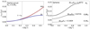Fig. 3 The amount of spin-up over time for clouds shaped as partial annuli and spheres. Left: simulated prograde spin-up of clouds in the shape of partial annuli that orbit around a central mass with (blue, SG) and without (red, NSG, Eq. (14)) self-gravity enabled. When self-gravity and collisions are included, the prograde spin-up levels off around the free-fall timescale (plotted here for an equivalent sphere), when cloud shear comes to a halt. Right: same calculation, computed with spherical clouds and varying initial densities. Their initial rotation scales as L0 ∝ (Rcl/RH)2, whereas the prograde spin-up during their collapse scales as Lrot ∝ (Rcl/RH)5 (see Sect. 2.3). As a result, sparse clouds with Rcl ≃ RH accumulate most of their rotation during their collapse, whereas the rotation of denser clouds remains largely unchanged.

3 Numerical Evaluation of Cloud Collapse in Orbit

In this section, we perform numerical simulations of cloud collapse in orbit, using the N-body code REBOUND (Rein & Liu 2012). The settings and numerical convergence of the runs are explained in detail in Appendix A. First, we numerically demonstrate the validity of our main analytical findings. Next, we present a second geometrical argument where the relative position of cloud particles, rather than their shared center-of-mass, is used to illustrate the prograde spin-up during a gravitational collapse.

3.1 Comparison With Analytical Formulation

The main simplification of our analytical example, besides its fixed two-dimensional geometry, is that it approximates the pro-grade spin-up without accounting for the orbital changes induced by self-gravity. In the left panel of Fig. 3, we numerically compute the same example including self-gravity to illustrate the spin-up of a cloud that actually collapses. The two curves initially follow the same trend of δL_rot ∝ t² during the early phase of the collapse. Then, the spin-up of the collapsing cloud begins to level off as it contracts sufficiently. The process of prograde spin-up eventually halts entirely when the cloud becomes a rigid body, and it can no longer shear out. Nevertheless, the analytical example provides a decent approximation when the spin-up is evaluated at t_ff.

Our analytical arguments predict that prograde spin-up scales as δL_rot ∝ (R_cl/R_H)⁵, more steeply than the cloud’s initial rotation, which scales as L₀ ∝ (R_cl/R_H)² (see Eqs. (14b), (16)). To test this trend and see if it holds for differently shaped clouds, we perform numerical simulations of uniform, spherical clouds with different initial sizes, again initialized on noneccentric, Keplerian orbits. We show the prograde spin-up of these runs in the right panel of Fig. 3 for initial cloud sizes between 0.5 and 1 R_H. As analytically predicted, the spin-up can exceed the initial rotation in scale, but only when the cloud nearly fills its Hill radius prior to collapse. Indeed, the fraction of accumulated rotation drops from δL_rot /L₀= 1.40 to δL_rot /L₀= 0.16 when the cloud’s initial size is halved. This factor of ~ 9 decline is similar to the factor of 8 predicted analytically and reiterates our finding that, while the rotation of dense (R_cl ≪ R_H) clouds remains largely unchanged during their collapse, clouds that fill their Hill sphere prior to collapse gain a substantial prograde component to their spins.

3.2 Prograde Spin-up in the Absence of Initial Rotation

It is also possible to visualize the prograde spin-up during a gravitational collapse in orbit by tracking the relative motion of a cloud’s inner- and outermost particles. A similar analysis was performed by Artem’ev & Radzievskii (1965) to show that a circular patch of material in Keplerian motion has prograde spin, a fact that also follows from the positive vorticity. We expand upon it here to illustrate the prograde spin-up of a cloud over time.

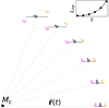Fig. 4 Orbital evolution of two noninteracting particles and their center-of-mass, initiated without rotation. Over time, both the interior (magenta arrow) and the exterior (orange arrow) particles start to revolve around their mutual center-of-mass (black arrow) in a prograde fashion, as shown by the angular displacement that develops relative to the horizontal dashed line. The quadratic prograde spin-up over time is additionally shown in the inserted panel, with the rotation at the different snapshots depicted by the black dots.

3.2.1 Two-particle Dynamics Without Self-gravity

The prograde spin-up during collapse is most striking in clouds that have no initial rotation, which we ensure by initiating all particles with (vector) velocities equal to that of their shared center-of-mass (see Appendix C). Prior to showing the rotational build-up in an N-body collapse, we first illustrate the underlying process in Fig. 4, where we consider the orbital motion of two horizontally aligned, noninteracting particles in a stationary frame. Their shared center-of-mass coordinate is shown with a black arrow and is initiated with a noneccentric Keplerian velocity.

Rather than focusing on the inward shift of the center-of-mass shift due to shear, which is not always visible relative to the cloud’s scale, we focus here on the relative motion of the particles. The innermost particle is more tightly bound to the central mass and traces out an elliptical orbit that is characterized by a greater angular velocity (θ) than that of the outermost particle. As a result of the orbital geometry, where its y-coordinate is modulated by a factor sin(θ) in this stationary frame, the inner particle begins to drop below the exterior one. Consequently, it is seen to effectively wrap below their shared center-of-mass in a prograde fashion. This behavior is mirrored in reverse by the outer particle, whose angular velocity is lower and, therefore, wraps around their center-of-mass from the top, again producing a prograde rotation. We emphasize this relative movement visually in Fig. 4 with a horizontal dashed line, drawn through the center-of-mass. In the inserted panel, the rotation relative to the center-of-mass is seen to rise quadratically over time, producing the same trend of prograde spin-up as a derived in Sect. 2.

3.2.2 N-body Collapse of A Spherical Cloud

We now perform a cloud collapse, using the same initial condition without rotation, but this time for a uniformly packed cloud with size R_H and with self-gravity and collisions enabled in REBOUND. We visualize the evolution of the collapsing cloud in Fig. 5¹, again shown in a stationary frame. If we compare the stages of collapse over time with Fig. 4, we observe that the general behavior remains unchanged. The difference is caused by the addition of self-gravity, which draws all particles toward their shared center-of-mass over time. In the intermediate stages of the collapse, this self-gravity reshapes the cloud into an aligned bar, as is the case when any rotating spheroid collapses Lin et al. (1965). Just like in the two-particle example, the interior particle drops below the center-of-mass – while those exterior remain above it. As the cloud contracts further and self-gravity intensifies, this prograde wrapping of particles on either side of the center-of-mass translates into a real prograde rotation of the object that forms.

4 Application: The Streaming Instability

We highlight the streaming instability as a small-scale example of a scenario where particle clouds form and then collapse due to their self-gravity while subject to a strong external force, in this case gravity from a central star. Streaming instabilities occur when small over-densities in the proto-planetary disk locally accelerate the gas, producing dense filaments where small solids concentrate and collapse to form planetesimals (Youdin & Goodman 2005; Johansen et al. 2007, 2009). Hydrodynamic simulations of the streaming instability in the proto-Kuiper belt have shown that it is possible to create equal-mass binaries in this manner (Nesvorný et al. 2010), which naturally seem to form with a strong preference for prograde rotation (Nesvorný et al. 2019, 2021). These simulations provide a striking agreement with the observed abundance of prograde, equal-mass binaries in the dynamically cold class of Kuiper belt objects (Noll et al. 2008; Fraser et al. 2017; Grundy et al. 2019).

In this section, we evaluate whether the mechanism of pro-grade spin-up can drive this bias in rotational direction. Similar to Robinson et al. (2020), we model the final collapse stage of the streaming instability with N-body simulations, and do not investigate the hydrodynamic onset of the instability itself, which sets the initial conditions for the collapse. Instead, we take a range of representative initial conditions and calculate the rotational gain in each of these scenarios. The effect of gas drag in this final collapse phase can be neglected for our purposes here, assuming that the cloud has a dust-to-gas ratio exceeding unity (Nesvorný et al. 2010).

4.1 Binary Formation Criterion

We first examine how much rotational angular momentum is required to form a binary. If a spherical asteroid has a uniform density ρ_p, its moment of inertia for rotation is $I_{\text{p}}=\left(2/5\right)M_{\text{p}}{R}_{\text{p}}^2$. If the asteroid’s material strength is neglected – a reasonable assumption based on their low typical internal strengths (see e.g., Burns 1975; Degewij & Gehrels 1976; Carbognani 2017; Persson & Biele 2021) – its spin can at most reach the breakup limit of ${\omega }_{\text{crit}}=\sqrt{4\pi G{\rho }_{\text{p}}/3}$ (Pravec & Harris 2000). The amount of angular momentum contained in a single asteroid’s spin can then be written as a fraction of this limit: $$L_{\text{spin},\text{p}}=I_{\text{p}}{\omega }_{\text{spin}}$$(17a) $$\simeq 0.06L_{\text{H}}{\left(\frac{d}{\text{AU}}\right)}^{-\frac{1}{2}}{\left(\frac{M_{★}}{M_{\odot }}\right)}^{\frac{1}{6}}{\left(\frac{{\rho }_{\text{p}}}{1}\right)}^{-\frac{1}{6}}\frac{{\omega }_{\text{spin}}}{{\omega }_{\text{crit}}},$$(17b)

where ω_spin ≤ ω_crit. Any excess rotational angular momentum can be accounted for by ejecting a portion of the mass, or by forming a binary (with mass ratio x_b = M₁ /M₂ and separation a_b), rather than a single planetesimal. In the idealized case without mass ejection, the complete rotational angular momentum budget gets divided into two spin terms around the respective asteroid centers (that sum to L_spin,p1 + L_spin,p2 = L_spin,binary), as well as an orbital term for the motion of the binary around their shared center-of-mass (L_orb,binary). The spin component follows from the moments of inertia as: $$L_{\text{spin,binary}}=L_{\text{spin,p}}{\left(1+x_{\text{b}}\right)}^{-\frac{5}{3}}\left(1+x_{\text{b}}^{\frac{5}{3}}\right),$$(18)

while the orbital rotation around the binary’s center-of-mass can be calculated from their angular velocity $\left({\omega }_{\text{b}}=\sqrt{G{M}_{\text{p}}/a_{\text{b}}^2}\right)$: $$L_{\text{orb,binary}}=M_1{\omega }_{\text{b}}{a}_1^2+M_2{\omega }_{\text{b}}{a}_2^2$$(19a) $$=L_{\text{H}}\frac{x_{\text{b}}}{{\left(1+x_{\text{b}}\right)}^2}{\left(\frac{a_{\text{b}}}{R_{\text{H}}}\right)}^{\frac{1}{2}}.$$(19b)

Assuming that the collapse forms a bound system of at most two objects, the sum of Eqs. (18) and (19b) specifies the possible binary configurations (x_b, a_b) for a given budget of rotational angular momentum. We examine these configurations in Fig. 6 at the location of the Kuiper belt (40 au) and at the inner edge of the main belt (1 au). The objects in the binaries are assumed to spin at breakup rate, in agreement with most Solar System asteroids (see e.g., Carbognani 2017; Persson & Biele 2021).

The first thing to note is that the formation of binaries is more likely at greater distances from the central star, where more angular momentum is available. This is due to the fact that the total rotational angular momentum generated in a collapse is constant across the disk in Hill units, which represent increasing angular momentum at greater orbital separations (L_H ∝ r₀). Furthermore, we note that the more equal the mass of the binary components, the more rotational angular momentum the combined system can store. When binaries are formed, therefore, they more commonly form with equal mass ratios in the outer disk. This trend is indeed reflected in the Solar System’s asteroid and comet population. In the next subsection, we take a closer look at the magnitude of the rotational accumulation with different initial conditions for the collapsing cloud.

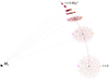Fig. 5 Overview of the collapse of a uniform cloud in orbit around a central mass, shown in a stationary frame. The spherical cloud is initiated with size RH and without any rotation. The snapshots from t = 0 to t = 0.8 ${\Omega }_0^{-1}$ are enlarged in scale for clarity. We highlight the positions and directions of two particles; one that is initiated closest to the central mass (magenta arrow) and one that starts the furthest away from the central mass (orange arrow). We also indicate the position and direction of the cloud’s center-of-mass (black edged arrow) and plot its initial distance (dark red semicircle). At the end of the collapse, the center-of-mass has shifted slightly inward toward the central mass, and the two particles have performed half a prograde revolution, confirming the prograde rotation of the object that is formed.

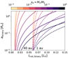Fig. 6 Possible binary configurations for a given rotational angular momentum budget (Lrot,binary) at two distances from the central star (40 au, solid; 1 au, dashed), assuming that the components themselves spin at near-breakup rates with density ρp = 1. When Lrot,binary < 0.06 LH, only single planetesimals are formed at 1 au as the breakup spin exceeds the angular momentum budget, whereas this critical value lies between 0.02 and 0.03 LH at 40 au. Large amounts of rotational angular momentum ≳0.1 LH can only be contained in binaries with increasingly wide mutual orbits and increasingly similar masses, especially in the outer disk.

4.2 Dependence of Spin-up on Initial Conditions

The magnitude of the prograde spin-up during a gravitational collapse depends on the initial conditions of the cloud, including its size (Sect. 3.1), velocity distribution and distance from the central star. We now examine the importance of the latter two variables by running an array of N-body collapses. We vary the semimajor axis between a₀ ∈ [10⁻¹, 10²] au and vary the cloud mass between the equivalent of planetesimals with radii R_p ∈ [10, 10³] km, assuming R_cl = R_H. We run this grid for four different rotational initial conditions for the cloud particles. Particles are either released on circular orbits referred to as the “Keplerian IC”, with the same velocity as their center-of-mass (“zero-rotation IC”), or with a uniform rotation relative to their center-of-mass (“uniform rotation IC”). For the latter we take the magnitude of the initial rotation equal to that of the Keplerian initial setup but now uniform and both prograde and retrograde. A detailed description of these initial conditions is given in Appendix C.

We show the results in Fig. 7, where we indicate the pro-grade spin-up as well as the corresponding inward shift in the semimajor axis. Consistent with our analytical prediction, the rotational build-up is both scale-invariant and distance-invariant when expressed in Hill units. As predicted, the reduction of the cloud’s semimajor axis during the collapse scales positively with the cloud mass and is proportional to its distance to the central star. Interestingly, the initial distribution of velocities in the cloud makes a large difference in the magnitude of the rotational gain. Whereas a cloud that begins with circular, Keplerian velocities attains an additional prograde rotation of δL_rot ≃ 0.15 L_H, clouds that begin with uniform rotation only gained δL_rot ≃ 0.05 L_H. This difference can be explained by the fact that prograde spin-up is driven by shear between the particles. If the initial conditions reflect more uniform motion, the cloud shears out to a less extended arc during the collapse and the rotational gain is reduced. Nevertheless, even clouds that start without any rotation accumulate a substantial prograde value of L_rot ≃ 0.05 L_H, which is enough to trigger unequal-mass binary formation outside a few astronomical units. In the case of Keplerian initial conditions, the rotational gain (to total L_rot ≃ 0.25 L_H) is enough to form equal-mass binaries across the proto-planetary disk (see Fig. 6).

5 Discussion

The mechanism of prograde spin-up is generally applicable to the gravitational contraction of any clouds that are subject to an external, central force. In any context, the key observational signature of this mechanism is a preferential alignment between the spin and orbital vectors of the objects that form. However, the rotational gain scales steeply as δL_rot ∝ (R_cl/R_H)⁵, such that only clouds whose sizes are set by the interplay of tidal shear and self-gravity (R_cl ~ R_H) experience significant spin-up when they collapse. Expressed in terms of a spherically uniform density, the pre-collapse system should not be much denser than ${\rho }_{\text{H}}=9M_C/\left(4\pi r_0^3\right)$, offering a scale-dependent benchmark. In this section, we will first compare our simple simulations of binary asteroid formation by streaming instability to other works. Next, we move up on the scale ladder and discuss the potential implications of prograde spin-up for the rotation of planets, stars and molecular clouds.

5.1 Comparison to Hydrodynamic Simulations of Binary Formation in the Kuiper Belt

We presented a simple application of prograde spin-up to the streaming instability, where we used a set of idealized initial conditions to show how perturbations by Solar gravity provide enough rotation to form prograde binary systems. In reality, such clouds have morphologies and velocity distributions that are set in a more complex manner by interactions between the nebular gas and the solids, including back-reactions (Youdin & Goodman 2005; Johansen et al. 2007, 2009). These processes were accounted for in more detail in the works by Nesvorný et al. (2019, 2021), who simulated the onset of the instability and initial stages of collapse using the hydrodynamics code ATHENA (Stone et al. 2008), prior to simulating high-resolution binary formation in the final collapse stage with the N-body code PKDGRAV (Stadel 2001). Notably, Nesvorný et al. (2019, 2021) exclude stellar gravity in their PKGRAV simulations, but include it in their ATHENA runs, allowing their results to be influenced by prograde spin-up during the key early collapse stage. A comparison with their results illustrates two points: First, the broad distribution of scaled angular momenta that is generated by their ATHENA simulations, both in magnitude and direction, emphasizes the importance of modeling the onset of the streaming instability when considering the initial conditions of the collapse. Second, the fact that our simple model replicates their key result, namely the tendency of streaming instabilities to form prograde binaries, indicates that the mechanism of prograde spin-up may well drive the rotational outcome in both models. Indeed, this suggestion is reinforced by the data shown in the supplementary Fig. 4 of Nesvorný et al. (2019), which indicates that the colatitude distribution of the vorticity vectors in their simulations is initially broad, and that the prograde bias only appears when the bound clumps collapse to form binary systems. We suggest that the relative importance of prograde spin-up to the turbulence of the instability determines the amount of prograde bias.

Rather than investigate the precise morphologies of these binary systems that form in SI, as was done with high-resolution studies by Robinson et al. (2020) and Nesvorný et al. (2021), we studied the mechanism behind the rotational evolution of material during the collapse. Conveniently, the prograde spin-up is largely independent of the chosen resolution or physical parameters such as coefficient of restitution and the particle size (see Appendix A). We should note, however, that the possibility of material ejection during the late stages of collapse means that not all the rotational angular momentum built up by the material necessarily ends up in the binary. The details tend to be more sensitive to parameter variations Robinson et al. (2020); Nesvorný et al. (2021), and high-resolution simulations remain necessary to study the precise configurations that can form.

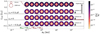Fig. 7 Prograde spin-up in the collapse phase of the streaming instability, visualized for a wide range of orbital separations, asteroid sizes and initial conditions. The dashed horizontal lines tangent to the circles represent the rotation prior to collapse, while the arrows indicate the magnitude of prograde spin-up. The ringed circles represent the size of the asteroid that forms, and their colors show the total center-of-mass displacement during the collapse δa. The systems within the dark red lines represent cases where there is insufficient rotational angular momentum to form binaries (ωspin < ωcrit). The systems above and below the red lines show the formation of prograde and retrograde binaries, respectively. The preference for prograde binary formation is clearly visible, especially in the outer disk.

5.2 Relevance of Prograde Spin-up During Planet Formation

At the scale of planets, the mechanism of prograde spin-up is most clearly applicable to the formation of giant planets by gravitational instability (see e.g., Kuiper 1951; Cameron 1978; Boss 1998). The spins of these large planets on wide orbits are only just beginning to be uncovered, with the only two currently known cases pointing to moderate or large obliquities (Bryan et al. 2020, 2021). Recent SPH and hydrodynamical simulations of gas giant formation, which are sensitive to prograde spin-up, indicate that gravitoturbulent disks can yield obliquities up to 90 degrees (Jennings & Chiang 2021), although most objects seem form with more alignment (Hall et al. 2017). One notable difference with asteroid formation is that a collapse that forms a gas giant is halted by gas pressure, rather than collisions between solids. In both cases, however, these arresting forces become relevant only when the collapse is almost complete and significant prograde spin-up has already taken place. Alternatively, in the framework of core accretion (see e.g., Mizuno 1980), gas giants could have accreted most of their mass and prograde angular momentum during the stage of runaway gas accretion (Machida et al. 2008; Dittmann 2021). In this case too, the nebular gas accretes onto the planet from a range of noneccentric orbits while exposed to stellar gravity, allowing for prograde spin-up to increase planetary rotation. Further work is required to resolve the statistical spin distribution of this class of planets and to investigate the role that prograde spin-up plays in setting their rotation.

The relevance of prograde spin-up to the formation of terrestrial planets is yet more difficult to assess. While their embryos may have formed in streaming instabilities, terrestrial planets likely accreted most of their mass and rotation from nearby planetesimals (see e.g., Pollack et al. 1996), from the aerodynamic capture of pebbles (Ormel & Klahr 2010; Lambrechts & Johansen 2012), or possibly from late giant impacts (see e.g., Wetherill 1985; Canup 2012). Seen from a rotational perspective, however, none of these scenarios seem to offer satisfactory explanations for the scale or prograde bias of planetary spins. The accretion of planetesimals fails to deliver sufficient rotation (Lissauer & Kary 1991; Dones & Tremaine 1993a) while stochastic, giant impacts lead to isotropic spin distributions (Safronov 1966; Dones & Tremaine 1993b). Pebble accretion has been found to produce large, prograde rotation in some regimes (Johansen & Lacerda 2010; Visser et al. 2020), although this may be dampened when protoplanetary envelopes are accounted for. There is, however, an alternative formation scenario that does involve a terrestrial-scale gravitational collapse. In the inside-out formation channel suggested by Chatterjee & Tan (2014); Hu et al. (2016, 2018); Mohanty et al. (2018); Cai et al. (2022), terrestrial cores are proposed to form out of dense pebble traps at the edges of dead zones. If planet formation indeed sometimes proceeds through this channel, the rotation of the planets it produces will likely be affected by prograde spin-up.

5.3 Prograde Spin-up of Molecular Clouds and Stars

Star formation is a hierarchical process that involves collapse on different scales, with potential applications for prograde spin-up at different levels. The process begins with the formation of a molecular cloud, the largest of which are observed to be concentrated toward galactic spiral arms (Lee et al. 2001; Blitz & Rosolowsky 2005; Stark & Lee 2005), where they form out of the interstellar medium, likely via gravitational instability driven by both stars and gas (Ballesteros-Paredes et al. 2007). At this scale, prograde spin-up is driven by the gravitational potential of the galaxy and contributes to an alignment between the rotation of the molecular cloud and its galactic orbit. Observations of molecular clouds in M 33 and M 51 confirm this trend, with strong measured prograde biases in their rotation (Braine et al. 2018, 2020). It is not clear what fraction of their rotation can be attributed to prograde spin-up, though, as both M 33 and M 51 have rising velocity curves that naturally lead to prograde rotation when a section of the disk contracts. Interestingly, Jeffreson et al. (2020) performed numerical simulations of molecular cloud formation in the dynamical galactic environment and found that the prograde bias remains even when the galactic rotation curve is declining and shear is expected to yield retrograde orbits. This persisting prograde bias fits the mechanism of prograde spin-up, but more work is required to investigate a potential connection. Moving down in scale, most stars are known to form in dense, gravitationally bound substructures within molecular clouds (see e.g., McKee & Ostriker 2007; Lee et al. 2012; Lee & Hennebelle 2016b), often referred to as star-forming clumps. When these clumps collapse and fragment, they form proto-clusters which often contain many thousand stars (see e.g., McKee & Ostriker 2007; Lee et al. 2012; Lee & Hennebelle 2016b). For the stars that form, the gravity from the star-forming clump itself acts as the external, central force necessary for prograde spin-up, which will act to align the angular momentum of the stellar spin (or binary orbit) with any orbital angular momentum within the cluster. While the available angular momentum is expected to reduce during star formation via magnetic breaking, the sign of the spin is maintained. If a star-forming clump contains systematic rotation, a spin-orbit alignment will translate to a correlation between the stellar spins in the cluster. Until recently, there had been no evidence of such a correlation, and the first spectroscopic studies of the young, low-mass open clusters Pleiades and Alpha Per were observed to be isotropic (Jackson & Jeffries 2010; Jackson et al. 2018). However, recent astroseismological measurements have shown that red giants in the higher-mass clusters NGC 6791 and NGC 6819 exhibit a strong inter-cluster spin alignment (Corsaro et al. 2017), pointing to an imprint of spin-orbit alignment during their formation. Hydrodynamic simulations indicate that this spin-alignment can indeed arise when the star-forming clumps are mostly rotationally supported prior to their global collapse (Lee & Hennebelle 2016a; Corsaro et al. 2017), though further numerical simulations that track the rotational evolution during the key early collapse of the star-forming clump are required to assess the relative importance that prograde spin-up plays in this process.

6 Conclusions

Larger asteroids, planets, stars in some clusters, as well as molecular clouds seem to possess a preferential alignment between their spins and orbital vectors, hinting at a shared link to their parent structures. In this work, we describe a process that can cause spin-orbit alignment based on the gravitational collapse of clouds in orbit around an external, central potential. We perform illustrative analytical and N-body calculations to show that a cloud’s rotational angular momentum relative to its center-ofmass is not conserved when it contracts next to such a potential, even if no material is ejected. Instead, because particles in a cloud shear away from one another over time – and do so on curved paths – their combined center-of-mass moves inward toward the source of the potential (See Fig. 2). The orbital angular momentum that is thus liberated, adds a prograde component to the spin of the object that forms. Equivalently, the process of spin-up can be understood from the prograde wrapping of inner and outer particles around the cloud’s center-of-mass, which we visualize in both a stationary (Figs. 4 and 5) and corotating (Fig. D.1) frame. The basic properties of the prograde spin-up mechanism are as follows:

1. Clouds that orbit around external, central potentials build up prograde rotation when they collapse due to self-gravity. The spin-up develops quadratically over time (δL_rot/L_H ∝ t²), before slowing down when the collapse completes (t ~ t_ff).

2. We find that the total rotational gain scales as $\delta L_{\text{rot}}/L_{\text{H}}\propto t_{\text{ff}}^2\propto {\left(R_{\text{cl}}/R_{\text{H}}\right)}^5$. The fifth-order scaling means that prograde spin-up is more important for clouds with lower densities prior to their collapse.

3. If the external potential is generated by a point mass and the initial cloud is spherical, we find a total increase in rotational angular momentum around δL_rot ≃ 0.05−0.15 $M_{\text{cl}}{\Omega }_0{R}_{\text{cl}}^2$. Out of the studied initial conditions, the magnitude of prograde spin-up is greatest when the cloud’s particles orbit with circular velocities prior to the collapse, allowing for efficient tidal shearing.

When applied to the Solar System, we suggest that this mechanism of prograde spin-up provides an explanation for the observed spin-orbit alignment of trans-Neptunian binaries (Grundy et al. 2019), provided that they formed in streaming instabilities (Youdin & Goodman 2005; Johansen et al. 2007, 2009). As such, prograde spin-up could operate to drive the recent simulation results of Nesvorný et al. (2019, 2021), who recently replicated this preferential spin-orbit alignment. The relevance of prograde spin-up to the formation of objects by gravitational collapse on larger astrophysical scales remains open for further investigation. It is likely, however, that the universal applicability of prograde spin-up contributes to the ubiquity of spin-orbit alignment on different scales. Compared to the rotation contained in shear: L_rot/L_H ∝ (R_cl/R_H)², prograde spin-up becomes important when the size of the cloud prior to collapse is comparable to the Hill radius. For objects that form in this interface between self-gravity and shear, prograde spin-up naturally produces a spin-orbit alignment, even in an environment of retrograde shear.

Acknowledgments

We are deeply indebted to Carsten Dominik and Amy Bonsor for their support and mentorship. We thank Chris Ormel and Helong Huang for providing comments and corrections. In addition, we are grateful for useful discussions on this topic with Mark Wyatt, Cathie Clarke, Elliot Lynch, Tess Roovers, Sjoerd van der Heijden, Mitchell Yzer, Tom Konijn, and Alexander Hackett. We thank the anonymous referee for an encouraging report. RGV acknowledges funding from the Dutch Research Council, ALWGO/15-01. MGB acknowledges the support of a Royal Society Studentship, RG 16050.

Appendix A Rebound Settings and Convergence

In this appendix, we describe the settings of our REBOUND runs used to model cloud collapse in the final stage of the streaming instability. First, we spread the particles evenly across the clouds to ensure that their density is uniform. To do so, we employ a Voronoi (Voronoi 1908) algorithm with Lloyd iterations (Lloyd 1982) until a high level of uniformity is achieved. The N-body integration itself is done with the variable step solver IAS 15 (Rein & Spiegel 2015).

As the clouds contract, particles begin to collide. We model these collisions with an inflated particle approach to reduce the number of numerical particles (N_n) from the number of physical particles (N_p). In this approach, the radius of the numerical particles (s_n) is blown up to maintain total cross section: s_n = s_p(N_p/N_n)^1/2. An interesting convenience that follows from the larger particles, as pointed out by Rein et al. (2010), is that the use of a gravitational softening parameter becomes redundant. We note that the inflated particle approach is only valid if the initial volume filling factor of the particles is well below the size of the cloud prior to collapse, in our simulations typically set to the Hill radius. Because the Hill radius is proportional to the orbital separation, the filling factor of a cloud with otherwise identical parameters (N_n, s_p) is reduced when it is positioned further from the star. In order to ensure that the cloud collapse behaves in the same manner at every semimajor axis, we instead fix the initial volume filling factor at f = 10⁻³ in every simulation. This stylized approach is not suitable for resolving the physical system that forms from a collapse, as was modeled by Robinson et al. (2020); Nesvorný et al. (2021), but it is suitable for gauging the total amount of spin-up during the collapse. It allows for the use of far fewer numerical particles while maintaining convergence in this result. We show this in Fig. A.1, where the obtained rotation is indeed not dependent on the chosen number of numerical particles nor on the choice of filling factor. The coefficient of restitution in our model is taken to be zero, a choice that was not found to influence the results.

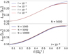Fig. A.1 Dependence of the prograde spin-up over time on numerical parameters. Top: variation of the filling factor of the simulation box between 10−4 ≤ f ≤ 10−1. The runs correspond to Nn = 5000 numerical particles and are run at 5 AU. Bottom: variation of the number of numerical particles 103 ≤ Nn ≤ 104, computed with a filling factor of f = 10−3. The magnitude of prograde spin-up is found to be insensitive to these numerical parameters.

Appendix B Angular Momentum Transformation Between Local Rotating and Inertial Frames

In local simulations such as the comoving frame with/without shearing sheet approximation, particle positions and velocities are determined in a frame that is both rotating and translated relative to the star. In order to calculate the rotation vector of a cloud from these quantities, it is necessary to transform the vectors correctly to an inertial frame with the origin located on the studied object. The results of such a transformation for circular orbits are given in 3D without derivation by Nesvorný et al. (2019) and in 1D by Giuli (1968); Dones & Tremaine (1993a). As far as we are aware, only a limited 1D justification is shown by Lissauer & Kary (1991). Because we could not find a complete 3D derivation of the required transformation anywhere, we provide it here.

Let the first, comoving frame with Cartesian coordinates (x, y, z) be centered at a (vector) distance r₀ of a central object, in a frame that is rotating around the central object with the rotation vector ${\Omega }_0={\Omega }_0\widehat{z}$. Let the second frame with Cartesian coordinates (x′, y′, z′) share its origin with the first frame but be stationary (inertial). In order to transform a vector from the first to the second frame, the following operations are required. First the frame is translated such that the origin coincides with the center of the orbit: r → r + r₀. Then the frame is rotated around the origin with −Ω₀, such that the frame becomes inertial: v → V + Ω₀ × r. Finally the frame is translated back, such that the origin is again located at the center of the cloud: r + r₀ → r. Together, these transformations lead to the following distance and velocity vectors in the stationary frame: $$r^{\prime }=r$$(B.1a) $$v^{\prime }=v+{\Omega }_0\times \left(r+r_0\right).$$(B.1b)

The rotation of a particle is given by its velocity relative to the cloud’s center-of-mass. If the center-of-mass remains located on r₀, it corresponds to v′_cm = Ω₀ × r₀ and the specific rotational angular momentum of a particle is given by: $${l^{\prime }}_{\text{rot}}=r^{\prime }\times \left(v^{\prime }-{v^{\prime }}_{\text{cm}}\right)$$(B.2a) $$=r\times \left(v-{\Omega }_0\times r\right)$$(B.2b) $$=\left(\begin{array}{c}y{\upsilon }_{\text{x}}-z{\upsilon }_{\text{y}}-{\Omega }_{0}xz\\ z{\upsilon }_{\text{x}}-x{\upsilon }_z-{\Omega }_{0}yz\\ x{\upsilon }_{\text{y}}-y{\upsilon }_{\text{x}}+{\Omega }_0\left(x^2+y^2\right)\end{array}\right).$$(B.2c)

This final equation can trivially be generalized to any direction of Ω₀ by using nonzero xy-components in Eq. B.2b. We note that there is, however, a potential issue with this calculation in a comoving frame. If the center-of-mass of the cloud shifts inward by a significant distance, the transformation no longer uses the right reference point for the rotation, as the object forms on a slightly interior orbit. The magnitude of this error grows with δR/r₀ ∝ (R_clΩ₀t/r₀)² (see Eq. 9b) and is not quantitatively important in the calculations performed in this work.

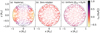Fig. B.1 Quiver plot of initial velocities in the comoving frame for three setups used in this paper. While our simulations use spherical clouds, this plot shows their cross sections at z=0. The arrow sizes correspond to the magnitude of the particle velocities and the colors correspond to the rotational contribution (from Eq. B.2c). The left panel (a) indicates the Keplerian setup (C.1), which yields a total prograde rotation equal to $L_{\text{rot}}\simeq 0.1M_{\text{cl}}{R}_{\text{cl}}^2$. The middle panel (b) corresponds to the zero-rotation initial condition (Eq. C.2), while the right panel (c) corresponds to uniform rotation with the same initial rotational angular momentum as the Keplerian setup.

Appendix C Initial Rotational Condition of Spherical Clouds

In Sects. 3 and 4.1, we perform collapse simulations with spherical clouds that start with three different velocity setups, which we explain here. We refer to the first setup we use as Keplerian, meaning that all particles in the cloud begin with velocities in the stationary frame (whose axes directions at t = 0 coincide with a corotating frame) equal to: $${v^{\prime }}_{\text{Keplerian}}\left(t=0\right)=\Omega \times r.$$(C.1)

We show these velocities translated to a comoving frame in panel (a) of Fig. B.1. In this frame, the velocity differences are mainly visible as shear $\left({\upsilon }_{\text{y}}\simeq -\frac{3}{2}{\Omega }_{0}x\right)$ on the x-axis. From Eq. B.2c, it is easy to see that the rotational contribution of particles on the x-axis becomes retrograde due to this shear, ranging from 0 to $-0.5{\Omega }_0{R}_{\text{cl}}^2$. On the y-axis, however, the shear is negligible and absolute velocity differences are minimal. Nevertheless, the curvature of the orbit (captured in the term Ω₀(x² + y²)) provides significant directional differences in velocity, which lead to pro-grade rotational contributions ranging from 0 to ${\Omega }_0{R}_{\text{cl}}^2$. When integrated over the complete sphere, the net initial rotational condition of the Keplerian setup is around $L_{\text{rot}}\simeq 0.1M_{\text{cl}}{\Omega }_0{R}_{\text{cl}}^2$.

We refer to the second setup used in this work as the zero-rotation condition. In this setup, we set all the velocities equal to $${v^{\prime }}_{\text{zero-rotation}}\left(t=0\right)={\Omega }_0\times r_0,$$(C.2)

such that all particles begin with the same velocity as a particle that is located at the sphere’s center-of-mass and orbits in a circular motion. Without velocity differences, the particles in the cloud have no initial rotation. However, this is not immediately visibly apparent in the corotating frame (panel (b) of Fig. B.1), where the velocities are transformed (Eq. B.1b). Even though the particles provide no physical rotational angular momentum, their rotation visibly appears to start in a retrograde condition in this frame with a rotational period equal to the orbital period.

Finally, the third setup we use in this paper is one with a uniform cloud rotation rate (ω_rot) where the initial velocities are set equal to: $${v^{\prime }}_{\text{uniform}}\left(t=0\right)={\Omega }_0\times r_0+{\omega }_{\text{rot}}\times \left(r-r_0\right).$$(C.3)

The initial rotational condition in this setup trivially follows as $L_{\text{rot}}=I_{\text{cl}}{\omega }_{\text{rot}}=0.4M_{\text{cl}}{\omega }_{\text{rot}}{R}_{\text{cl}}^2$. In Fig. B.1, we plot the velocities in a corotating frame for the case where ω_rot = Ω₀/4 and the initial rotational angular momentum is identical to the Keplerian setup. In the special case where ω_rot = Ω₀ is chosen, all the particles appear stationary in the comoving frame.

Appendix D Collapse of A Spherical Cloud in A Comoving Frame

In Fig. D.1, we repeat the collapse of an initially nonrotating spherical cloud in orbit (same calculation as Fig. 5), visualized instead in the commonly used corotating frame - rather than a stationary one. In this frame, the curvature of the orbital motion that is naturally present in a stationary frame is instead introduced by the Coriolis acceleration. In the first panel, the nonrotating cloud visually appears to have a retrograde rotation, which is a consequence of the noninertiality of the frame (see also Fig. B.1(b)). As the cloud shears out and contracts, it again first attains a barlike shape. When the particles are pulled toward the center-of-mass, they wrap around it in a prograde fashion. Finally, the collapse finishes and a spherical object with pro-grade rotation has formed. The physical shape and multiplicity of the system that forms, depends on the numerical parameters assumed, such as the filling factor and number of numerical particles. Importantly, however, the rotational direction and its magnitude remain unaffected by these numerical parameters.

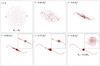Fig. D.1 Overview of the collapse of a uniform cloud in orbit around a central mass (same as Fig. 5), shown in a comoving frame. The spherical cloud is initiated with size RH and without any rotation. The central mass is located left from the cloud. The velocity directions (magnitudes not to scale) and trajectory of the particles are highlighted for an interior and exterior particle that both wrap around the center-of-mass in a prograde fashion.

References

All Figures

Fig. 1 Schematic setup of our analytical calculation (Sect. 2). We consider a two-dimensional cloud of mass Mcl in a stationary frame, whose origin lies on the central mass MC ≫ Mcl (where the dotted lines cross). The initial shape of the cloud is that of a partial annulus, bounded by inner and outer circles with radii r0 ± Rcl and radial lines at angles ±θ0. We follow the position $\left({\overline{x}}_{\text{cl}},{\overline{y}}_{\text{cl}}\right)$ and velocity $\left({\overline{\upsilon }}_{\text{x,cl}},{\overline{\upsilon }}_{\text{y,cl}}\right)$ of the cloud’s center-of-mass over time and calculate the specific rotational angular momentum of cloud particles $\left(\widehat{z}\right)$ relative to this point as $l_{\text{rot}}=\left(x{\upsilon }_{\text{y}}-y{\upsilon }_{\text{x}}\right)-\left({\overline{x}}_{\text{cl}}{\overline{\upsilon }}_{\text{y,cl}}-{\overline{y}}_{\text{cl}}{\overline{\upsilon }}_{\text{x,cl}}\right)$, shown in the color plot at t = 0. The initial velocities of the cloud particles correspond to circular, Keplerian motion. Particles that start on the x-axis initially contribute retrograde rotation due to shear, whereas particles on the y-axis contribute prograde rotation due to curvature. The integrated result is a net initial prograde rotational angular momentum that increases over time if the cloud orbits freely (see Eq. (14b)).

In the text

	Fig. 2 Illustration of the inward center-of-mass shift in our analytical example. The particles follow circular orbits around a central mass without mutual interactions. As the particles shear out over time, the ensemble deforms into an increasingly extended single arc, shifting the center-of-mass position (open circular dot) closer to the orbital midpoint.
In the text

Fig. 3 The amount of spin-up over time for clouds shaped as partial annuli and spheres. Left: simulated prograde spin-up of clouds in the shape of partial annuli that orbit around a central mass with (blue, SG) and without (red, NSG, Eq. (14)) self-gravity enabled. When self-gravity and collisions are included, the prograde spin-up levels off around the free-fall timescale (plotted here for an equivalent sphere), when cloud shear comes to a halt. Right: same calculation, computed with spherical clouds and varying initial densities. Their initial rotation scales as L0 ∝ (Rcl/RH)2, whereas the prograde spin-up during their collapse scales as Lrot ∝ (Rcl/RH)5 (see Sect. 2.3). As a result, sparse clouds with Rcl ≃ RH accumulate most of their rotation during their collapse, whereas the rotation of denser clouds remains largely unchanged.

In the text

Fig. 4 Orbital evolution of two noninteracting particles and their center-of-mass, initiated without rotation. Over time, both the interior (magenta arrow) and the exterior (orange arrow) particles start to revolve around their mutual center-of-mass (black arrow) in a prograde fashion, as shown by the angular displacement that develops relative to the horizontal dashed line. The quadratic prograde spin-up over time is additionally shown in the inserted panel, with the rotation at the different snapshots depicted by the black dots.

In the text

Fig. 5 Overview of the collapse of a uniform cloud in orbit around a central mass, shown in a stationary frame. The spherical cloud is initiated with size RH and without any rotation. The snapshots from t = 0 to t = 0.8 ${\Omega }_0^{-1}$ are enlarged in scale for clarity. We highlight the positions and directions of two particles; one that is initiated closest to the central mass (magenta arrow) and one that starts the furthest away from the central mass (orange arrow). We also indicate the position and direction of the cloud’s center-of-mass (black edged arrow) and plot its initial distance (dark red semicircle). At the end of the collapse, the center-of-mass has shifted slightly inward toward the central mass, and the two particles have performed half a prograde revolution, confirming the prograde rotation of the object that is formed.

In the text

Fig. 6 Possible binary configurations for a given rotational angular momentum budget (Lrot,binary) at two distances from the central star (40 au, solid; 1 au, dashed), assuming that the components themselves spin at near-breakup rates with density ρp = 1. When Lrot,binary < 0.06 LH, only single planetesimals are formed at 1 au as the breakup spin exceeds the angular momentum budget, whereas this critical value lies between 0.02 and 0.03 LH at 40 au. Large amounts of rotational angular momentum ≳0.1 LH can only be contained in binaries with increasingly wide mutual orbits and increasingly similar masses, especially in the outer disk.

In the text

Fig. 7 Prograde spin-up in the collapse phase of the streaming instability, visualized for a wide range of orbital separations, asteroid sizes and initial conditions. The dashed horizontal lines tangent to the circles represent the rotation prior to collapse, while the arrows indicate the magnitude of prograde spin-up. The ringed circles represent the size of the asteroid that forms, and their colors show the total center-of-mass displacement during the collapse δa. The systems within the dark red lines represent cases where there is insufficient rotational angular momentum to form binaries (ωspin < ωcrit). The systems above and below the red lines show the formation of prograde and retrograde binaries, respectively. The preference for prograde binary formation is clearly visible, especially in the outer disk.

In the text

Fig. A.1 Dependence of the prograde spin-up over time on numerical parameters. Top: variation of the filling factor of the simulation box between 10−4 ≤ f ≤ 10−1. The runs correspond to Nn = 5000 numerical particles and are run at 5 AU. Bottom: variation of the number of numerical particles 103 ≤ Nn ≤ 104, computed with a filling factor of f = 10−3. The magnitude of prograde spin-up is found to be insensitive to these numerical parameters.

In the text

Fig. B.1 Quiver plot of initial velocities in the comoving frame for three setups used in this paper. While our simulations use spherical clouds, this plot shows their cross sections at z=0. The arrow sizes correspond to the magnitude of the particle velocities and the colors correspond to the rotational contribution (from Eq. B.2c). The left panel (a) indicates the Keplerian setup (C.1), which yields a total prograde rotation equal to $L_{\text{rot}}\simeq 0.1M_{\text{cl}}{R}_{\text{cl}}^2$. The middle panel (b) corresponds to the zero-rotation initial condition (Eq. C.2), while the right panel (c) corresponds to uniform rotation with the same initial rotational angular momentum as the Keplerian setup.

In the text

Fig. D.1 Overview of the collapse of a uniform cloud in orbit around a central mass (same as Fig. 5), shown in a comoving frame. The spherical cloud is initiated with size RH and without any rotation. The central mass is located left from the cloud. The velocity directions (magnitudes not to scale) and trajectory of the particles are highlighted for an interior and exterior particle that both wrap around the center-of-mass in a prograde fashion.

In the text

References

- Alibert, Y. 2017, A&A 606, A69 [NASA ADS] [CrossRef] [EDP Sciences] [Google Scholar]
- Artem’ev, A. V., & Radzievskii, V. V. 1965, Sov. Astron. 9, 96 [Google Scholar]
- Ballesteros-Paredes, J., Klessen, R. S., Mac Low, M. M., & Vazquez-Semadeni, E. 2007, in Protostars and Planets V, eds. B. Reipurth, D. Jewitt, & K. Keil (Tucson: University), 63 [Google Scholar]
- Belloche, A. 2013, EAS Pub. Ser. 62, 25 [NASA ADS] [CrossRef] [EDP Sciences] [Google Scholar]
- Benecchi, S. D., Noll, K. S., Grundy, W. M., et al. 2009, Icarus 200, 292 [NASA ADS] [CrossRef] [Google Scholar]
- Benecchi, S. D., Noll, K. S., Stephens, D. C., Grundy, W. M., & Rawlins, J. 2011, Icarus 213, 693 [NASA ADS] [CrossRef] [Google Scholar]
- Blitz, L., & Rosolowsky, E. 2005, Astrophys. Space Sci. Lib. 327, 287 [NASA ADS] [CrossRef] [Google Scholar]
- Boss, A. P. 1998, ApJ 503, 923 [Google Scholar]
- Boss, A. P. 2021, ApJ 911, 146 [NASA ADS] [CrossRef] [Google Scholar]
- Bottke, W. F., Durda, D. D., Nesvorný, D., et al. 2005a, Icarus 175, 111 [Google Scholar]
- Bottke, W. F., Durda, D. D., Nesvorný, D., et al. 2005b, Icarus 179, 63 [Google Scholar]
- Braine, J., Rosolowsky, E., Gratier, P., Corbelli, E., & Schuster, K. F. 2018, A&A 612, A51 [NASA ADS] [CrossRef] [EDP Sciences] [Google Scholar]
- Braine, J., Hughes, A., Rosolowsky, E., et al. 2020, A&A 633, A17 [NASA ADS] [CrossRef] [EDP Sciences] [Google Scholar]
- Brouwers, M. G., Ormel, C. W., Bonsor, A., & Vazan, A. 2021, A&A 653, A103 [NASA ADS] [CrossRef] [EDP Sciences] [Google Scholar]
- Bryan, M. L., Chiang, E., Bowler, B. P., et al. 2020, AJ 159, 181 [Google Scholar]
- Bryan, M. L., Chiang, E., Morley, C. V., Mace, G. N., & Bowler, B. P. 2021, AJ 162, 217 [NASA ADS] [CrossRef] [Google Scholar]
- Burns, J. A. 1975, Icarus 25, 545 [NASA ADS] [CrossRef] [Google Scholar]
- Cai, M. X., Tan, J. C., & Portegies Zwart, S. 2022, MNRAS 510, 5486 [NASA ADS] [CrossRef] [Google Scholar]
- Cameron, A. G. W. 1978, Moon Planets 18, 5 [Google Scholar]
- Canup, R. M. 2012, Science 338, 1052 [NASA ADS] [CrossRef] [Google Scholar]
- Carbognani, A. 2017, Planet. Space Sci. 147, 1 [NASA ADS] [CrossRef] [Google Scholar]
- Caselli, P., Benson, P. J., Myers, P. C., & Tafalla, M. 2002, ApJ 572, 238 [Google Scholar]
- Chatterjee, S., & Tan, J. C. 2014, ApJ 780, 53 [Google Scholar]
- Corsaro, E., Lee, Y.-N., García, R. A., et al. 2017, Nat. Astron. 1, 0064 [NASA ADS] [CrossRef] [Google Scholar]
- Davis, D. R., Weidenschilling, S. J., Farinella, P., Paolicchi, P., & Binzel, R. P. 1989, in Asteroids II, eds. R. P. Binzel, T. Gehrels, & M. S. Matthews (Tucson: University of Arizon Press), 805 [Google Scholar]
- Degewij, J., & Gehrels, T. 1976, BAAS 8, 459 [NASA ADS] [Google Scholar]
- Dittmann, A. J. 2021, MNRAS 508, 1842 [NASA ADS] [CrossRef] [Google Scholar]
- Dones, L., & Tremaine, S. 1993a, Icarus 103, 67 [NASA ADS] [CrossRef] [Google Scholar]
- Dones, L., & Tremaine, S. 1993b, Science 259, 350 [NASA ADS] [CrossRef] [Google Scholar]
- Fleck, R. C. J., & Clark, F. O. 1981, ApJ, 245, 898 [NASA ADS] [CrossRef] [Google Scholar]
- Fraser, W. C. 2009, ApJ 706, 119 [NASA ADS] [CrossRef] [Google Scholar]
- Fraser, W. C., Bannister, M. T., Pike, R. E., et al. 2017, Nat. Astron. 1, 0088 [NASA ADS] [CrossRef] [Google Scholar]
- Giuli, R. T. 1968, Icarus 8, 301 [NASA ADS] [CrossRef] [Google Scholar]
- Goldreich, P., & Peale, S. J. 1968, ARA&A 6, 287 [NASA ADS] [CrossRef] [Google Scholar]
- Goldreich, P., & Ward, W. R. 1973, ApJ 183, 1051 [Google Scholar]
- Grundy, W. M., Noll, K. S., Roe, H. G., et al. 2019, Icarus 334, 62 [CrossRef] [Google Scholar]
- Hall, C., Forgan, D., & Rice, K. 2017, MNRAS 470, 2517 [NASA ADS] [CrossRef] [Google Scholar]
- Hoyle, F. 1951, in Problems of Cosmical Aerodynamics (USA: IAU Symp.), 195 [Google Scholar]
- Hu, X., Zhu, Z., Tan, J. C., & Chatterjee, S. 2016, ApJ, 816, 19 [Google Scholar]
- Hu, X., Tan, J. C., Zhu, Z., et al. 2018, ApJ 857, 20 [NASA ADS] [CrossRef] [Google Scholar]
- Jackson, R. J., & Jeffries, R. D. 2010, MNRAS 402, 1380 [NASA ADS] [CrossRef] [Google Scholar]
- Jackson, R. J., Deliyannis, C. P., & Jeffries, R. D. 2018, MNRAS 476, 3245 [NASA ADS] [CrossRef] [Google Scholar]
- Jeffreson, S. M. R., Kruijssen, J. M. D., Keller, B. W., Chevance, M., & Glover, S. C. O. 2020, MNRAS 498, 385 [Google Scholar]
- Jennings, R. M., & Chiang, E. 2021, MNRAS 507, 5187 [NASA ADS] [CrossRef] [Google Scholar]
- Johansen, A., & Lacerda, P. 2010, MNRAS 404, 475 [NASA ADS] [Google Scholar]
- Johansen, A., & Nordlund, Å. 2020, ApJ 903, 102 [NASA ADS] [CrossRef] [Google Scholar]
- Johansen, A., Oishi, J. S., Low, M., et al. 2007, Nature 448, 1022 [Google Scholar]
- Johansen, A., Youdin, A., & Mac Low, M.-M. 2009, ApJ 704, L75 [NASA ADS] [CrossRef] [Google Scholar]
- Kuiper, G. P. 1951, Proc. Natl. Acad. Sci. 37, 1 [NASA ADS] [CrossRef] [Google Scholar]
- Lambrechts, M., & Johansen, A. 2012, A&A 544, A32 [NASA ADS] [CrossRef] [EDP Sciences] [Google Scholar]
- Lee, Y.-N., & Hennebelle, P. 2016a, A&A 591, A30 [NASA ADS] [CrossRef] [EDP Sciences] [Google Scholar]
- Lee, Y.-N., & Hennebelle, P. 2016b, A&A 591, A31 [NASA ADS] [CrossRef] [EDP Sciences] [Google Scholar]
- Lee, Y., Stark, A. A., Kim, H.-G., & Moon, D.-S. 2001, ApJS 136, 137 [NASA ADS] [CrossRef] [Google Scholar]
- Lee, E. J., Murray, N., & Rahman, M. 2012, ApJ 752, 146 [NASA ADS] [CrossRef] [Google Scholar]
- Lin, C. C., Mestel, L., & Shu, F. H. 1965, ApJ 142, 1431 [NASA ADS] [CrossRef] [Google Scholar]
- Lissauer, J. J., & Kary, D. M. 1991, Icarus 94, 126 [NASA ADS] [CrossRef] [Google Scholar]
- Lissauer, J. J., & Safronov, V. S. 1991, Icarus 93, 288 [NASA ADS] [CrossRef] [Google Scholar]
- Lloyd, S. 1982, IEEE Trans. Inf. Theor. 28, 129 [CrossRef] [Google Scholar]
- Machida, M. N., Kokubo, E., Inutsuka, S.-I., & Matsumoto, T. 2008, ApJ, 685, 1220 [NASA ADS] [CrossRef] [Google Scholar]
- Marsset, M., Fraser, W. C., Bannister, M. T., et al. 2020, Planet. Sci. J. 1, 16 [NASA ADS] [CrossRef] [Google Scholar]
- McKee, C. F., & Ostriker, E. C. 2007, ARA&A 45, 565 [Google Scholar]
- Medeiros, H., Lazzaro, D., & Kodama, T. 2018, Planet. Space Sci. 160, 77 [NASA ADS] [CrossRef] [Google Scholar]
- Mestel, L. 1966, MNRAS 131, 307 [NASA ADS] [CrossRef] [Google Scholar]
- Mizuno, H. 1980, Prog. Theor. Phys. 64, 544 [NASA ADS] [CrossRef] [Google Scholar]
- Mohanty, S., Jankovic, M. R., Tan, J. C., & Owen, J. E. 2018, ApJ 861, 144 [Google Scholar]
- Morbidelli, A., Bottke, W. F., Nesvorný, D., & Levison, H. F. 2009, Icarus 204, 558 [Google Scholar]
- Nesvorný, D., Youdin, A. N., & Richardson, D. C. 2010, AJ 140, 785 [Google Scholar]
- Nesvorný, D., Li, R., Youdin, A. N., Simon, J. B., & Grundy, W. M. 2019, Nat. Astron. 3, 808 [CrossRef] [Google Scholar]
- Nesvorný, D., Li, R., Simon, J. B., et al. 2021, Planet. Sci. J. 2, 27 [CrossRef] [Google Scholar]
- Noll, K. S., Grundy, W. M., Chiang, E. I., Margot, J. L., & Kern, S. D. 2008. Binaries in the Kuiper Belt (Tucson: University of Arizona Press), 345 [Google Scholar]
- Ormel, C. W., & Klahr, H. H. 2010, A&A 520, A43 [NASA ADS] [CrossRef] [EDP Sciences] [Google Scholar]
- Pan, M., & Sari, R. 2005, Icarus 173, 342 [NASA ADS] [CrossRef] [Google Scholar]
- Peebles, P. J. E. 1969, ApJ 155, 393 [Google Scholar]
- Persson, B. N. J., & Biele, J. 2021, ArXiv e-prints [arXiv:2110.15258] [Google Scholar]
- Pirogov, L., Zinchenko, I., Caselli, P., Johansson, L. E. B., & Myers, P. C. 2003, A&A 405, 639 [NASA ADS] [CrossRef] [EDP Sciences] [Google Scholar]
- Pollack, J. B., Hubickyj, O., Bodenheimer, P., et al. 1996, Icarus 124, 62 [NASA ADS] [CrossRef] [Google Scholar]
- Pravec, P., & Harris, A. W. 2000, Icarus 148, 12 [NASA ADS] [CrossRef] [Google Scholar]
- Pravec, P., Harris, A. W., Vokrouhlický, D., et al. 2008, Icarus 197, 497 [NASA ADS] [CrossRef] [Google Scholar]
- Rein, H., & Liu, S. F. 2012, A&A 537, A128 [NASA ADS] [CrossRef] [EDP Sciences] [Google Scholar]
- Rein, H., & Spiegel, D. S. 2015, MNRAS 446, 1424 [Google Scholar]
- Rein, H., Lesur, G., & Leinhardt, Z. M. 2010, A&A 511, A69 [NASA ADS] [CrossRef] [EDP Sciences] [Google Scholar]
- Renaud, F., Bournaud, F., Emsellem, E., et al. 2013, MNRAS 436, 1836 [NASA ADS] [CrossRef] [Google Scholar]
- Rey-Raposo, R., & Read, J. I. 2018, MNRAS 481, L16 [NASA ADS] [CrossRef] [Google Scholar]
- Rey-Raposo, R., Dobbs, C., & Duarte-Cabral, A. 2015, MNRAS 446, L46 [NASA ADS] [CrossRef] [Google Scholar]
- Robinson, J. E., Fraser, W. C., Fitzsimmons, A., & Lacerda, P. 2020, A&A 643, A55 [EDP Sciences] [Google Scholar]
- Rubincam, D. P. 2000, Icarus 148, 2 [Google Scholar]
- Safronov, V. S. 1962, Prob. Cosmog. 8, 177 [NASA ADS] [Google Scholar]
- Safronov, V. S. 1966, Sov. Astron. 9, 987 [NASA ADS] [Google Scholar]
- Safronov, V. S. 1972, Evolution of the Protoplanetary Cloud and Formation of the Earth and Planets (Jerusalem: Keter Publishing House) [Google Scholar]
- Schäfer, B. M. 2009, Int. Jo. Mod. Phys. D 18, 173 [CrossRef] [Google Scholar]
- Schäfer, U., Yang, C.-C., & Johansen, A. 2017, A&A 597, A69 [Google Scholar]
- Shmidt, 0.1. 1957, Chetyre lektsii O treorii proiskhozhdeniia Zemli. (Izdatel’stvo AN SSSR) [Google Scholar]
- Simon, J. B., Armitage, P. J., Li, R., & Youdin, A. N. 2016, ApJ 822, 55 [Google Scholar]
- Stadel, J. G. 2001, PhD thesis, University of Washington, USA [Google Scholar]
- Stark, A. A., & Lee, Y. 2005, ApJ 619, L159 [CrossRef] [Google Scholar]
- Steinberg, E., & Sari, R. 2015, AJ 149, 124 [NASA ADS] [CrossRef] [Google Scholar]
- Stone, J. M., Gardiner, T. A., Teuben, P., Hawley, J. F., & Simon, J. B. 2008, ApJS 178, 137 [NASA ADS] [CrossRef] [Google Scholar]
- Visser, R. G., Ormel, C. W., Dominik, C., & Ida, S. 2020, Icarus 335, 113380 [NASA ADS] [CrossRef] [Google Scholar]
- Voronoi, G. 1908, Journal für die reine und angewandte Mathematik (Crelles Journal) 1908, 198 [CrossRef] [Google Scholar]
- Wetherill, G. W. 1985, Science 228, 877 [NASA ADS] [CrossRef] [Google Scholar]
- Youdin, A. N., & Goodman, J. 2005, ApJ 620, 459 [Google Scholar]
- Youdin, A. N., & Shu, F. H. 2002, ApJ 580, 494 [NASA ADS] [CrossRef] [Google Scholar]
Figure 5 shows the collapse in a stationary frame that is centered on a much more massive central mass. This poses the visual difficulty that any collapsing cloud is tiny in comparison to the scale of its orbit. To circumvent this, we place subpanels at the corresponding center-of-mass positions where we zoom in. The cloud scale is, therefore, exaggerated for clarity but the collapse evolution is still visualized in a stationary frame.