| Issue |
A&A
Volume 663, July 2022
|
|
|---|---|---|
| Article Number | A1 | |
| Number of page(s) | 12 | |
| Section | Extragalactic astronomy | |
| DOI | https://doi.org/10.1051/0004-6361/202142031 | |
| Published online | 01 July 2022 | |
Impact of very massive stars on the chemical evolution of extremely metal-poor galaxies
1
SISSA, Via Bonomea 265, 34136 Trieste, Italy
e-mail: sgoswami@sissa.it
2
INAF-OATs, Via G. B. Tiepolo 11, 34143 Trieste, Italy
3
IFPU – Institute for Fundamental Physics of the Universe, Via Beirut 2, 34014 Trieste, Italy
4
CENTRA, Instituto Superior Técnico, Av. Rovisco Pais 1, 1049-001 Lisboa, Portugal
5
Dipartimento di Fisica e Astronomia, Università degli studi di Padova, Vicolo Osservatorio 3, Padova, Italy
6
Instituto de Astronomia Teorica y Experimental (IATE), Consejo Nacional de Investigaciones Cientificas y Tecnicas de la Republica Argentina (CONICET), Argentina
7
IRA-INAF, Via Gobetti 101, 40129 Bologna, Italy
8
INFN, Sezione di Padova, Via Marzolo 8, 35131 Padova, Italy
9
INAF – Osservatorio Astronomico di Padova, Vicolo dell’Osservatorio 5, 35122 Padova, Italy
10
CIERA and Department of Physics & Astronomy, Northwestern University, Evanston, IL 60208, USA
11
Dipartimento di Fisica e Astronomia, Università degli Studi di Bologna, Via Gobetti 93/2, 40129 Bologna, Italy
Received:
16
August
2021
Accepted:
2
May
2022
Context. In recent observations of extremely metal-poor, low-mass, starburst galaxies, almost solar Fe/O ratios are reported, despite N/O ratios consistent with the low metallicity.
Aims. We aim to investigate if the peculiar Fe/O ratios can be a distinctive signature of an early enrichment produced by very massive objects dying as pair-instability supernova (PISN).
Methods. We ran chemical evolution models with yields that account for the contribution by PISN. We used both the non-rotating stellar yields from a recent study and new yields from rotating very massive stars calculated specifically for this work. We also searched for the best initial mass function (IMF) that is able to reproduce the observations.
Results. We can reproduce the observations by adopting a bi-modal IMF and by including an initial burst of rotating very massive stars. Only with a burst of very massive stars can we reproduce the almost solar Fe/O ratios at the estimated young ages. We also confirm that rotation is absolutely needed to concomitantly reproduce the observed N/O ratios.
Conclusions. These results stress the importance of very massive stars in galactic chemical evolution studies and strongly support a top-heavy initial mass function in the very early evolutionary stages of metal-poor starburst galaxies.
Key words: galaxies: abundances / galaxies: starburst / galaxies: formation / stars: massive / galaxies: structure
© S. Goswami et al. 2022
 Open Access article, published by EDP Sciences, under the terms of the Creative Commons Attribution License (https://creativecommons.org/licenses/by/4.0), which permits unrestricted use, distribution, and reproduction in any medium, provided the original work is properly cited.
This article is published in open access under the Subscribe-to-Open model. Subscribe to A&A to support open access publication.
1. Introduction
The study of local metal-poor galaxies can greatly help to shed light on early galaxy evolution since they are expected to represent a significant baryon component in the early Universe. Extremely metal-poor galaxies (EMPGs), with metallicities less than 12+log(O/H) = 7.69 (Kunth & Östlin 2000; Izotov et al. 2012; Isobe et al. 2021, 2022), 12+log(O/H) = 8.69 being the solar metallicity (Asplund et al. 2009), are a particular example of this class that has been discovered both in the local Universe and at high redshifts. Local EMPGs have low stellar masses (log(M⋆/M⊙) ∼ 6–9) and high specific star formation rates (i.e., SFR per unit stellar mass, sSFR ∼ 10–100 Gyr−1) (Izotov & Thuan 1998; Thuan & Izotov 2005; Pustilnik et al. 2005; Izotov et al. 2009, 2018, 2019; Skillman et al. 2013; Hirschauer et al. 2016; Hsyu et al. 2017). They are considered as the analogues of high-z galaxies, with similar metallicities and low stellar masses discovered at redshift z ∼ 2−3 (Christensen et al. 2012a,b; Vanzella et al. 2017) and z ∼ 6−7 (Stark et al. 2017; Mainali et al. 2017).
Recently, a new EMPG survey called the Extremely Metal-Poor Representatives Explored by the Subaru Survey (EMPRESS, Kojima et al. 2020) was initiated with wide-field optical imaging data obtained with the Subaru/Hyper Suprime-Cam (HSC; Miyazaki et al. 2018) and Subaru Strategic Program (HSC/SSP; Aihara et al. 2018). In particular, Kojima et al. (2021) presented element abundance ratios of local EMPGs from EMPRESS and the literature. They found that neon- and argon-to-oxygen abundance ratios (Ne/O, Ar/O) are similar to those of known local dwarf galaxies, and that the nitrogen-to-oxygen abundance ratios are lower than ∼20% of the solar N/O value, in agreement with the low oxygen abundance. Regarding the iron-to-oxygen abundance ratios Fe/O, they found that their metal-poor galaxies show a decreasing trend in Fe/O ratio as metallicity increases, which is similar to what was found in the star-forming sample of Izotov et al. (2006), but with two representative EMPGs with exceptionally high Fe/O ratios at the low metallicity end. In Kojima et al. (2021), three scenarios that might explain the observed Fe/O ratios of their EMPGs are described, as summarised in the following.
The first scenario is based on the preferential dust depletion of iron (Rodríguez & Rubin 2005; Izotov et al. 2006). In this case, it is assumed that the gas-phase Fe/O abundance ratios of the EMPGs decrease with metallicity because Fe is depleted into dust more efficiently than O; this depletion becomes important at higher metallicities, when dust production is more efficient. However, Kojima et al. (2021) do not find evidence that galaxies with a larger metallicity have a larger colour excess, that is they are dust richer. Hence, the Fe/O decrease of their sample should not be due to dust depletion, and thus they exclude this scenario.
The second scenario invokes the presence of metal enrichment and gas dilution due to inflow. In this case, it is assumed that metal-poor galaxies formed from metal-enriched gas with solar metallicity and Fe/O ratio. Then, if primordial gas falls onto metal-enriched galaxies, the metallicity (inferred by the oxygen abundance O/H) decreases, whereas the Fe/O ratio does not change. This scenario might explain the almost solar Fe/O ratios, but one would expect an almost solar N/O ratio as well; the two peculiar EMPGs with high Fe/O ratios have low N/O ratios (lower than 20% of the solar value), which is at variance with what would have been expected by this second scenario, that should therefore be ruled out.
Finally, the third scenario refers to the contribution of super massive stars. Ohkubo et al. (2006) showed that stars with masses larger than ∼300 M⊙ can produce a large amount of iron during supernova (SN) explosion, and hence Kojima et al. (2021) suggested that this contribution of iron could result in the high Fe/O ratios of the two peculiar EMPGs. In this case, the N/O ratio would not be affected by a SN explosion, as required by observations (Iwamoto et al. 1999; Ohkubo et al. 2006).
While the latter scenario by Kojima et al. (2021) is appealing, other possible solutions could be conceived, especially those that take into account the detailed chemical evolution of the elements in the environmental conditions of such galaxies. There is a large amount of literature on the chemical evolution of galaxies, and in particular on the mechanisms that may give rise to the different abundance ratios observed in the Milky Way (MW) and in nearby galaxies (e.g., Matteucci 2021, and reference therein).
Concerning metal-poor galaxies, relevant progress to explain the observed spread in abundance ratios of selected elements such as He, N, and O has been made with the introduction of differential outflows, i.e., with the assumption that the ejecta of SNII may leave the potential well of the galaxies more efficiently than the ejecta of intermediate- and low-mass stars (e.g., Pilyugin 1993; Marconi et al. 1994), or even that different SNII ejecta may escape with different efficiencies via the so-called selective winds (e.g., Mac Low & Ferrara 1999; Recchi et al. 2001, 2008; Fujita et al. 2004; Ott et al. 2005; Recchi & Hensler 2007; Salvadori et al. 2008, 2014, 2019). In particular, Recchi et al. (2008) showed that variations of abundance ratios, including [O/Fe], could indeed be obtained by assuming different relative efficiencies in the outflows of the O and Fe ejected from SNe, but that such differences are unlikely to happen in the early phases of a starburst (Recchi et al. 2004), which are the typical condition of the EMPG galaxies we are analysing here.
Thus, in the following, we reconsider the scenario favoured by Kojima et al. (2021), with the help of new yields that include the effects of pulsational pair instability supernovae (PPISN) and pair instability supernovae (PISN, Goswami et al. 2021).
It is worth noting that PISN yields have already been included in the analysis of the chemical evolution of galaxies by other authors; however, this is with a motivated constraint that they should not be able to form above a certain threshold metallicity, Zcr ≲ 10−4 Z⊙ (Schneider et al. 2002; Salvadori et al. 2008). The reason for this choice is that detailed studies of the fragmentation process show that the characteristic fragment mass drops dramatically if the effects of the first formed dust are added to metal line cooling. In this case, typical fragments of solar or subsolar masses are obtained for any metallicity Z > Zcr (Schneider et al. 2006). Instead, if dust cooling does not operate, the same models predict typical final fragments of one hundred solar masses up to a metallicity of Zcr ≲ 10−2 Z⊙.
On the observational side, there has been compelling spectroscopic evidence (Crowther et al. 2016) of very massive single stars with initial masses up to about 300 M⊙ populating young starburst regions in the Large Magellanic Cloud (LMC). The spectroscopic VLT-FLAMES Tarantula Survey, which is monitoring the 30 Dor region in the LMC (Schneider et al. 2018a,b), has revealed the presence of single stars with ages between 1 and 6 Myr and a general mass distribution well populated up to 200 M⊙. Furthermore, the derived overall IMF of stars more massive than 15 M⊙ has a slope of x = 0.9 (x = 1.35 being the Salpeter one), with the individual region around NGC 2070 showing x = 0.65. The LMC has a typical metallicity of Z ∼ 0.3 M⊙ (Costa et al. 2019), much larger than the lower value of Zcr predicted by theoretical models. Some of these stars are already evolved, and, given their high surface helium content, they will likely be affected by the electron-pair creation instability process in their future evolution and end up as PPISN and/or PISN supernovae.
In terms of stellar evolution, only large mass-loss rates may prevent the formation of PISN by such massive stars. With the current models, the PISN fate is possible up to Z ∼ 0.5 Z⊙ (Kozyreva et al. 2014; Langer 2012; Costa et al. 2021), above which mass-loss rates are indeed strong enough to prevent this SN channel.
To overcome this tension between theory and observations, it has been argued that very massive objects (VMOs) might arise from early merging during their evolution, e.g., as members of interacting binaries. However, the young age of some of the most massive stars in the 30 Dor region does not favour a scenario in which all of them are the results of merger events (Crowther et al. 2016; Schneider et al. 2018a).
The effects of the PISN phase in the abundance ratios of EMPG galaxies can be tested using the recent models for non-rotating massive and very massive stars provided by Goswami et al. (2021), which include the contribution from PPISN and PISN. A peculiarity of the ejecta of PISN is the production of large amounts of Fe and O, in proportions that are strongly dependent on the He core mass at the end of the central H burning phase (Heger & Woosley 2002; Kozyreva et al. 2014; Takahashi et al. 2018). Chemical evolution models that include PISN yields may possess a very early phase with a low [O/Fe] and then rapidly evolve into the domain of the α-enhanced regime (Goswami et al. 2021). Based on these findings, we tested whether the high Fe/O together with the low N/O abundance ratios of EMPGs can both be explained using the yields of very massive stars or if additional ingredients are required.
The paper is structured as follows. In Sect. 2, we describe the simple chemical evolution model used in this work. In particular, to include the PISN yields, we needed to shift the upper mass limit of the IMF in the domain of very massive objects. In this section, we also discuss the PISN yields with particular emphasis on an update of the Goswami et al. (2021) tables that concern the effects of stellar rotation. In Sect. 3, we present the observational data that we wish to analyse. In Sect. 4, we compare the observations to the results of suitable chemical evolution models stressing the derived evolutionary constraints. In Sect. 5, we present our choice for a bi-modal IMF that, together with a model that includes a burst of rotating very massive objects, is able to reproduce the observations well. Finally, in Sect. 6, we summarise our conclusions.
2. Chemical evolution model
The chemical evolution code used in this work is CHE-EVO (Silva et al. 1998). This is a one-zone open chemical evolution model, which follows the time evolution of the gas abundances of elements, including infall of primordial gas. This code has been used in several contexts to provide the input star formation and metallicity histories to interpret the spectrophotometric evolution of both normal and starburst galaxies (e.g., Vega et al. 2008; Fontanot et al. 2009; Silva et al. 2011; Lo Faro et al. 2013, 2015; Hunt et al. 2019). The basic equation used in this code can be written as follows:
where, for the element j, the first term on the right,  , represents the rate of gas consumption by star formation,
  corresponds to the infall rate of pristine material and
  refers to the rate of gas return to the interstellar medium (ISM) by dying stars. The latter term also includes the contribution of type Ia supernovae (SNIa), whose rate is adjusted with the parameter ASNIa, which corresponds to the fraction of binaries with system masses between 3 M⊙ and 16 M⊙ and the right properties to give rise to SNIa (Matteucci & Greggio 1986).
We used the Schmidt–Kennicutt law (Kennicutt 1998) to model the star formation rate (SFR):
where ν is the efficiency of star formation, Mg is the mass of the gas, and k is the exponent of the star formation law. The gas infall law is assumed to be exponential (e.g., Grisoni et al. 2017, 2018), with an e-folding timescale of τinf. The IMF can be written as follows:
We used a Kroupa-like three-slope power-law IMF with x = 0.3 for 0.1 ≤ Mi/M⊙ ≤ 0.5, x = 1.2 for 0.5 ≤ Mi/M⊙ ≤ 1, and we change the upper mass limit (MUP) and the slope of the upper IMF (xUP) in the high-mass domain (Marks et al. 2012) to explore the importance of very massive stars in the chemical evolution of EMPGs.
The input parameters of the chemical evolution models considered in this work are summarised in Table 1. In the following, we give details on the stellar and nucleosynthesis models providing our adopted ejecta for the chemical evolution.
Input parameters of selected chemical evolution and yield models. MTW is our set of stellar ejecta described in Goswami et al. (2021).
For low- and intermediate-mass stars (Mi < 8 M⊙), we distinguish between single stars and binary systems that give rise to SNe Ia (Matteucci & Greggio 1986). For single stars with initial masses of Mi < 6 M⊙, we considered yields from calibrated asymptotic giant branch (AGB) models by Marigo et al. (2020). For 6 M⊙ < Mi < 8 M⊙, we considered super-AGB yields from Ritter et al. (2018). For SNIa, we used the yields provided by Iwamoto et al. (1999). For 8 M⊙ ≤ Mi ≤ 350 M⊙, we adopted the yield compilation by Goswami et al. (2021) for massive stars and very massive objects. They include stellar wind ejecta, based on the non-rotating PARSEC models (Bressan et al. 2012), and explosive ejecta carefully extracted from explosive models of electron-capture SN (ECSN; Wanajo et al. 2009), core-collapse supernova (CCSN; Chieffi & Limongi 2004), PPISN (Woosley et al. 2002; Chen et al. 2014; Yoshida et al. 2016; Woosley 2017), and PISN (Heger & Woosley 2002; Heger et al. 2003). The yields have been calculated for Zi = 0.0001, 0.001, 0.006, and 0.02. Though the ejecta of PISN are taken from the zero-metallicity models by Heger & Woosley (2002), they are very similar to those computed for initial metallicities of Zi = 0.001 by Kozyreva et al. (2014).
The effect of PISNe is apparent for Zi ≤ 0.001, with substantial production of O, Mg, Si, S, Ar, Ca, Ti, and Fe, due to C and O ignition within a collapsing core. For more details, we refer the reader to Goswami et al. (2021).
Concerning the concomitant low N/O ratios observed in these EMPGs, it is worth noting that nitrogen production by massive stars is strongly affected by rotation (Limongi & Chieffi 2018). In non-rotating massive-star models, nitrogen ejecta are much lower than those of rotating models because of extra mixing towards the external layers produced by rotation and subsequent dispersion by stellar winds (Limongi & Chieffi 2018; Grisoni et al. 2021). This is also true for the N ejecta by PISN, as it can be evaluated by comparing the new ejecta of very massive stars with and without rotation by Takahashi et al. (2018) in Fig. 1. Even in the case of PISN, nitrogen is essentially produced in the pre-supernova evolution.
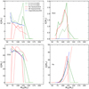 |
Fig. 1. C12, N14, O16, and Fe PISN yields from Z = 0.0001 rotational models of this work (green, solid, and dotted lines for 2 rotation rate values) based on pure He non-rotating models (blue) from Heger & Woosley (2002). In red, we show rotating (solid) and non-rotating (dotted) yields by Takahashi et al. (2018). We note that N14 yields from non-rotating models are negligible. |
To fully test the effect of PISN in both O and N production, we computed new yields with the latest PARSEC pre-supernova models with rotation from 100 M⊙ to 350 M⊙ up to the beginning of the PISN instability process, as described in Costa et al. (2021). We then extracted the explosive yields for Zi = 0.0001, 0.001, and 0.006 from the models by Heger & Woosley (2002) using the He core mass as the only parameter, as in Goswami et al. (2021). For the massive stars that do not enter the PISN channel (including the most massive stars with Zi = 0.02), we adopted the yields from Limongi & Chieffi (2018). A comparison of stellar ejecta from PISN models is shown in Fig. 1. The ejecta of selected elements from non-rotating PISN models (Heger & Woosley 2002) are shown in blue, while the corresponding ones obtained after matching the PARSEC rotating models are shown in green, and, finally, the ones for rotating and non-rotating models computed by Takahashi et al. (2018) are shown as red, solid, and dotted lines, respectively. By comparing the first two sets, we appreciate that the contribution of the pre-SN evolution, i.e., the excess of the green lines above the blue lines, are only significant for the light elements. In particular, we see that nitrogen production from the explosion is negligible with respect to the one arising from the pre-SN evolution. There are some differences with respect to ejecta of Takahashi et al. (2018), which are quite evident for nitrogen, silicon, and magnesium. For the former element, the reason must lie in the different assumptions for the pre-SN models. For the latter elements, the differences must reside in the explosion mechanism. In any case, for the other two elements relevant for this work (oxygen and iron), the different models provide results that are in fair agreement.
3. Observational data
The observational data considered in this work are taken from the Extremely Metal-Poor Representatives Explored by the Subaru Survey (EMPRESS, Kojima et al. 2020), which provides a database of sources based on the wide-field deep imaging of the Hyper Suprime-Cam Subaru Strategic Program (HSC-SSP) combined with wide-field shallow data of the SDSS. From this large programme, Kojima et al. (2020) selected a local (z ≲ 0.03) sample of EMPGs, i.e., of small galaxies with properties similar to those of high-z galaxies in the early star formation phase (low M⋆, high sSFR, low metallicity, and young stellar ages) through a machine-learning classifier trained with model templates of galaxies, stars, and QSOs to distinguish EMPGs from other types of objects.
For ten of the selected candidates, they conducted spectroscopy follow-ups to infer their detailed physical quantities. Their ten analysed sources are confirmed as EMPGs, due to active SF as witnessed by strong emission lines with rest frame HβEWs > 100 Å, stellar masses of log(M⋆/M⊙) = 5.0−7.1, high specific star formation rates of ∼300 Gyr−1, young stellar ages ∼50–100 Myr, and low metallicities. In particular, three of these sources strictly satisfy their EMPG criterion of 12+log(O/H) < 7.69, i.e., Z < 0.1 Z⊙, with HSC J1631+4426 showing the lowest metallicity value ever reported, 12+log(O/H) = 6.90 (i.e., Z/Z⊙ = 0.016). The other sources still show very low metallicities (∼0.1−0.6 Z⊙).
For nine of these selected objects, Kojima et al. (2021) also provided elemental abundance ratios (Fe/O, N/O, Ne/O, Ar/O) and completed their sample with another EMPG, J0811+4730 (Izotov et al. 2018), from the literature, which has the second lowest reported metallicity (0.0019 Z⊙). This is the same sample of ten local EMPGs we considered in our analysis, with the two extreme EMPGs (HSC J1631+4426 and J0811+4730) requiring specific modelling in order to interpret their abundance ratios. In particular, the ionising radiation of half of the sampled objects, including these lowest metallicity galaxies, has been found by Kojima et al. (2021) to show both high He II λ4686/Hβ ratios (> 1/100) together with the high Hβ EW (> 100 Å). They ascribe these large values to hard radiation from VMOs, which is also their preferred explanation for the exceptionally high Fe/O ratios for some of their objects, as summarised in the introduction.
In Fig. 2, we show the Fe/O (left panel) and N/O (right panel) ratios versus the metallicity 12+log(O/H) for these ten EMPGs (empty and filled circles). In the left panel, a sample of Galactic thick- and thin-disc stars (blue and magenta dots, Bensby et al. 2014) and low-metallicity stars (grey dots, Cayrel et al. 2004) are shown for comparison. In the right panel, the error bars as provided by Kojima et al. (2020) are of the size of the circles plotted in the figure. The light grey dots correspond to local galaxies from Izotov et al. (2006); the dark gray dots are assembled from Pettini et al. (2002) and Pettini et al. (2008), which are for extragalactic H II regions and high-redshift DLA systems.
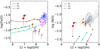 |
Fig. 2. Fe/O ratio (left panel) and N/O ratio (right panel) as a function of the metallicity, 12+log(O/H). EMPGs from Kojima et al. (2021) are shown as numbered circles from 1 to 9. Object 10 is the EMPG from Izotov et al. (2018). The lowest metallicity EMPGs are are highlighted as filled circles (red for objects 3 and 10, and orange for the intermediate object 6). In the left panel, blue and magenta dots represent, respectively, thin and thick disc stars from Bensby et al. (2014), and grey dots represent low-metallicity stars from Cayrel et al. (2004). In the right panel, light grey dots correspond to local galaxies from Izotov et al. (2006), and dark grey dots are assembled from Pettini et al. (2002) and Pettini et al. (2008), which are for extragalactic H II regions and high-redshift DLA systems. Solid line with squares show the evolution of the abundance ratios for the models of Table 1. The six squares mark, from left to right, model ages at 5, 20, 30 , 60, 100, and 200 Myr, respectively, the latter being larger than the estimated upper limit by Kojima et al. (2021). See text for details. |
4. Evolutionary constraints from the abundance ratios
In this section, we describe how we tested a number of different chemical evolution parameters to understand which evolution scenario is able to produce the high Fe/O ratios and, at the same time, to keep low N/O ratios, as observed in EMPGs 3, 10 and partly 6, which are the three galaxies selected as strictly belonging to the EMPG class.
Their peculiar Fe/O abundance ratio, with respect to other EMPGs of the sample and Galactic disc stars, is illustrated in the left panel of Fig. 2. To better highlight the peculiarity of these three EMPG galaxies, we begin by showing a reference model, M1, whose chemical evolution parameters are within the range of those adopted to reproduce the chemical evolution of the stars in the disc of the MW (Grisoni et al. 2017, 2018, 2019; Grisoni et al. 2020a; Spitoni et al. 2021; Goswami et al. 2021). Model M1 has a Kroupa et al. (1993) type IMF with a slope of xUP = 1.5 in the high-mass range and an upper mass limit of 100 M⊙, as shown in Table 1.
We see from Fig. 2, left panel, that this model is able to reproduce the location of the thin and thick disc stars of the MW fairly well (Bensby et al. 2014), as well as that of the tail of halo stars at a lower metallicity (Cayrel et al. 2004). We stress that this model is only used as a reference, because the different MW components, which are characterised by significantly different metallicity and age distributions, are actually reproduced by different sets of chemical evolution parameters (Goswami et al. 2021). From this figure, we may appreciate the peculiarity of EMPG 3 and EMPG 10. Their Fe/O values are clearly well above the region occupied by the other low-metallicity objects that, in this region, are almost all below model M1. EMPG 3 has a large error bar that makes it only marginally compatible with model M1. Instead, EMPG 6 could be well fitted by model M1 because, with 12+(O/H) ∼ 7.6, it falls in between the tail of low-metallicity stars (Cayrel et al. 2004; Bensby et al. 2014) that are reproduced by model M1. However, if we also consider the temporal evolution of model M1, we immediately see that this match is only apparent. To highlight this point, we marked six ages with superimposed squares along the M1 path: 5, 20, 30, 60, 100, and 200 Myr, from left to right, respectively.
Model M1 approaches the location of EMPG 6 at ∼0.5 Gyr. This age is about one order of magnitude larger than the maximum age value estimated for EMPGs from their spectro-photometric and nebular emission properties, as described in Sect. 3 (Kojima et al. 2020).
With model M1, we also checked the effect of maximising the Fe production, with respect to O, by setting ASNIa = 0.95. In this model, not shown here for the sake of clarity, the Fe/O ratio reaches, at maximum, a value close to object 6. Thus, even by increasing the SNIa fraction to almost the maximum allowed value, it is not possible to fit EMPGs 3 and 10. This is because the SNIa-enhanced model reaches the O/H values observed for these galaxies in about 100 Myr, a timescale that is too short to allow the evolution of the bulk of intermediate- and low-mass binary systems, which are the main Fe producers for the selected IMF. We thus confirm that, by using an IMF with a canonical MUP such as that of Kroupa et al. (1993), we cannot reproduce the two EMPGs with the highest Fe/O ratios.
The run of the N/O ratio is plotted in the right panel of Fig. 2. As can be seen from this figure, EMPGs 3, 10, and 6 do not show peculiar abundance ratios with respect to other low-metallicity objects. Nevertheless, model M1 is not able to reproduce the observed N/O ratios, as in the case of the stars of our Galaxy, which is discussed in Goswami et al. (2021). This is due to a lack of enough N production from non-rotating massive stars. It has recently been shown that one of the main effects of including rotation in the model of massive stars is that of increasing the N production, and indeed only models with rotation may be able to provide the primary N required to fit low-metallicity stars and extragalactic H II regions or high-redshift DLA systems (Pettini et al. 2002, 2008; Goswami & Prantzos 2000; Grisoni et al. 2021). We examine N production below.
4.1. The Fe/O ratio
We checked whether a different IMF could better reproduce the observed Fe/O ratios of EMPGs 3, 10, and 6. With a bottom heavier IMF, the resulting metal enrichment would be slower. This would not only exacerbate the age discrepancy already found for EMPG 6, but it would likely also increase this tension in the case of EMPG 3 and EMPG 10, whose O/H could be explained with model M1 at an age of about 100 Myr. We thus computed a model, M2, with a top heavier IMF, the same chemical evolution parameters as M1, but an IMF slope in the high-mass domain xUP = 0.6, all while keeping the same MUP = 100 M⊙. Model M2 is depicted in cyan in Fig. 2. As expected, M2 shows a faster metal enrichment than M1 and is able to reach the observed O/H value of EMPG 6 in less than 100 Myr.
However, increasing the fraction of massive stars with a flatter IMF results in a larger production of α-elements, with respect to Fe, and the Fe/O ratio drops significantly instead of increasing. Model M2 runs below model M1 and is not able to reproduce the observed Fe/O ratios of EMPGs 3, 10, and 6. It is, however, able to reproduce the low Fe/O values of the other EMPGs, at an age that is still compatible with that estimated from spectro-photometric and nebular properties of these galaxies.
As discussed earlier, one possibility to obtain the observed high Fe/O ratios could be by means of selective outflows, in the specific case a more efficient ejection for O than for Fe. However, as long as elements are produced by the same stars (massive) and on similar (short) timescales, as in the case of the young EMPGs we discuss here, then they should have comparable ejection efficiencies (Recchi et al. 2004). Furthermore, it has also been shown with both simple analytic and numerical models that if the yields do not depend on the metallicity, the models also evolve at constant abundance ratios if differential (i.e., with efficiency independent of the element) winds are assumed (Recchi et al. 2008). Thus, if the observed abundance ratios are those produced during the ongoing starburst phase, the high observed Fe/O ratios and the normal observed N/O ratios of EMPG 3 and EMPG 10 must be a consequence of the initial yield ratios (e.g., Eqs. (2) and (29) in Recchi et al. 2008).
In this respect, Fig. 1 shows that the ejecta from PISN, once integrated on a suitable IMF, may indeed be able to reproduce the observed abundance ratios.
Therefore, we now consider models that also include PISN ejecta, and for this purpose we need to extend MUP in the domain of very massive stars.
By adopting the ejecta from Goswami et al. (2021), the best model we can obtain with reasonable IMF values is model M3. It is characterised by a top-heavy IMF with xUP = 0.6 and MUP = 300 M⊙. Such a flat slope is close to the lowest value determined for the Arches star cluster (Marks et al. 2012) or for NGC 2070 in the 30 Dor star forming region (Schneider et al. 2018a). The Fe/O ratio predicted by model M3 is significantly higher than that obtained by all previous models. However, although it is fully compatible with the Fe/O ratio of EMPG 3, considering the large error bar for this object, model M3 falls too short to explain the large Fe/O observed for EMPG 10. We also note that model M3 is able to reach the (O/H) values of EMPG 3 and EMPG 10 in less than 30 Myr and that of EMPG 6 in less than 60 Myr.
Regarding what we previously stated, the young age obtained on one side justifies the omission of selective outflows, and on the other side renders the model quite independent of the assumed SNIa fraction.
Another evident characteristic of model M3 is the sharp drop of the Fe/O ratio when it reaches 12+log(O/H) ∼ 8. This cannot be a result of the intervening type Ia supernovae above about 60 Myr, because in that case the Fe/O ratio should have increased even further. Instead it is a clear evidence that the adopted ejecta are not metal independent. Indeed the Goswami et al. (2021) ejecta were computed by interpolating those by Heger & Woosley (2002) as a function of MHe and it is the relation between MHe and Mi that strongly depends on metallicity because of the adopted mass-loss rates. The general trend is that, at increasing metallicity and keeping MUP fixed, the upper IMF spans a decreasing range of MHe values until MHe becomes lower than the threshold to produce PISN. Given the dependence of the Fe and O ejecta from MHe, the model shows such a sharp drop in the Fe/O ratio. Thus, model M3 shows that a continuous burst of star formation actually evolves naturally towards a decreasing sequence that takes place when the metallicity reaches the stellar-evolution threshold for the PISNe production, i.e., that produced by large mass-loss rates. Since all the selected galaxies have high specific star formation rates and low total stellar masses and estimated young ages, it could also be that some of them form an ageing sequence of the starburst.
4.2. The N/O ratio
We then compared the N/O ratios as given by the same models M2 and M3 discussed for the Fe/O ratio with data. Model M2 performs even worse than model M1. Due to the absence of rotation in the yields, the primary N production is not well reproduced, similarly to M1. Moreover, due to the flatter IMF slope, N/O is lower than in M1, as O is produced more as explained above, and the model is only able to follow the secondary behaviour of N at higher metallicities. Given that N is not a product of the explosive phase and that the ejecta are those of non-rotating stars, model M3 behaves similarly to M2 but produces even lower N/O ratio values because PISN enhance the production of O without affecting that of N. None of the models we have tested so far is able to produce the observed N/O ratio at early times, i.e., at low metallicity.
It has recently been shown that only massive star models with rotation are able to produce and eject (even during their pre-supernova evolution) enough N to reproduce the N abundance pattern observed in metal-poor stars of the MW and in nearby galaxies (Limongi & Chieffi 2018; Prantzos et al. 2018; Grisoni et al. 2021). In fact, it has been shown that rotation is needed to reproduce the abundance patterns of other chemical elements in the MW besides nitrogen such as carbon (Romano et al. 2020) and fluorine (Grisoni et al. 2020b). Since this is also true for stars that end their life as PISN stars (Takahashi et al. 2018) and since these latter stars seem necessary to reproduce the high observed Fe/O ratio of EMPGs 3, 10, and 6, we computed new VMO models with rotation.
We remind the reader that, while the final O and Fe ejecta from PISN models are not significantly affected by the initial rotational velocity of the stars, the results are very different for N14, as shown in Fig. 1. We thus calculated several sets of VMO models at increasing rotational velocity, from 100 M⊙ to 350 M⊙ for Zi = 0.0001 and Zi = 0.001. The stellar models were followed from the pre-main sequence phase until the beginning of central oxygen burning, at which point they become unstable due to efficient electron-positron pair production. At this stage, N production by these stars ceases because the evolutionary timescales become very short and wind ejecta inefficient. The total ejecta are then obtained by adding the ejecta of explosive pure He models (Heger & Woosley 2002), matched by means of the PARSEC final He core mass. Starting from a negligible N production in non-rotating models, the N ejecta increase at increasing rotation, becoming significantly higher when the initial angular rotational velocity, Ω, reaches 60% of the critical one,  , the latter corresponding to the point where the centrifugal acceleration equals the gravitational one at the equator.
5. Chemical evolution models with a variable IMF
Besides the problem of the N abundance, even model M3, which includes the PISN yields, is not able to fully reproduce the high Fe/O ratios observed in EMPG 10. It also has a prolonged phase of relatively high Fe/O until a metallicity of 12+log(O/H) ∼ 8 is reached. Beyond this point, higher mass-loss rates caused by the high metallicity prevents stars with high He core mass from entering the domain of PISN, and Fe is no longer produced while O continues to be copiously ejected. To sample the effects of VMOs exploding as PISN, we include an early phase in our chemical evolution model, where the IMF has the following form:
![$$ \begin{aligned} \phi (M_{\rm i}) = \frac{\mathrm{d}n}{\mathrm{d}\log (M_{\rm i})} \propto M_{\rm i}^{-1.3}\times \mathrm{exp}\left[\,- \left(\, \frac{M_{\rm char}}{M_{\rm i}} \right)^{1.6}\right] ,\end{aligned} $$](/articles/aa/full_html/2022/07/aa42031-21/aa42031-21-eq8.gif)
with 80 M⊙ ≤ Mi ≤ 350 M⊙.
This distribution, originally devised by Chabrier (2003), was adopted by Wise et al. (2012) to describe the masses of population III stars, with a characteristic mass of Mchar = 40 M⊙. Here, we tested a few values of Mchar between Mchar = 200 M⊙ and Mchar = 300 M⊙, because the relative PISN ejecta of O and Fe strongly depend on their He core mass in the above range of initial masses (see Fig. 1).
This phase of PISN enrichment is confined to the early evolution of the starburst, defined by the gas metallicity being below a threshold metallicity of Zcr. Above Zcr, we adopted a Kroupa-like IMF, Eq. (3), with xUP = 1.3 and MUP = 40 M⊙.
With this bi-modal IMF, we tested two different values of the threshold metallicity, Zcr = 10−4 and 10−2 Z⊙. As discussed in the introduction, these values have been suggested by Schneider et al. (2006) and Salvadori et al. (2008), respectively, for the cases of efficient and inefficient dust cooling during the early star formation process.
The results are presented for yields obtained adopting stellar-evolution models with two different rotational parameters, ω = Ω/Ωcrit = 0.3 and 0.4 (because with these values we bracket the observed N/O ratios), and for Zcr = 10−4 (models M4ω3 and M4ω4) and Zcr = 10−2 (models M5ω3 and M5ω4). The other parameters of the chemical evolution models for the two Zcr values are reported in Table 2.
Chemical evolution model parameters and properties of the initial VMO burst when the gas metallicity reaches Z = Zcr.
The adopted bi-modal IMF is shown in Fig. 3. The VMO IMF, from 80 M⊙ to 350 M⊙ is normalised to the integral of the SFR from the beginning to the time when the total metallicity reaches the value Z = Zcr × Z⊙ for Zcr = 0.0001 (solid line) and Zcr = 0.01 (dashed line), respectively. This corresponds to the total mass of gas, converted into stars, Mcum, by the time Zcr is reached. The value of Mcum at Z/Z⊙ = Zcr is shown in Table 2 for the different chemical evolution models.
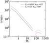 |
Fig. 3. Adopted IMF for chemical evolution of models M4ω4 (solid red line) and M5ω4 (dot-dashed red line). The VMO IMF distributions are given by Eq. (4) with Mchar = 200 M⊙ and normalised to the cumulative mass reached at the corresponding Zcr. For comparison, the IMFs of the post-VMO burst phases, with the same mass normalisation, are also shown (black lines). The expected number of VMOs is shown in the label and in Table 2. |
The total numbers of VMO stars that have been formed, NVMO, are indicated in the figures and reported in the last column of Table 2. After Zcr is reached, the IMF is changed to the Kroupa-like IMF. This is also plotted in Fig. 3, normalised to the corresponding value of Mcum reached at Zcr, for the sake of comparison. The last two columns in Table 2 refer to the number of VMOs at Z/Z⊙ = Zcr expected from a model whose total stellar mass equals the observed galaxy stellar mass, at the corresponding value of 12+log(O/H).
Figure 4 shows the early evolution of the metallicity of the starburst model M4ω4, for Zcr = 0.0001 (upper panel), and M5ω4, and Zcr = 0.01 (lower panel), both for Mchar = 200 M⊙. They are computed with the same yields obtained with PISN models with rotation parameter ω = 0.4. The models M4ω3 and M5ω3 , computed with lower rotational velocity, ω = 0.3, run very similarly to the previous ones and are not shown in the plot for the sake of simplicity.
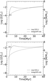 |
Fig. 4. Evolution of gas metallicity (solid lines) and cumulative mass converted into stars (dash-dotted lines) of models that include an early burst of VMOs exploding as PISN. The threshold metallicity for VMO formation is Zcr = 10−4 (M4ω4, upper panel) and 10−2 (M5ω4, lower panel). Their IMF distribution is shown in Fig. 3. In both panels the adopted Mchar is 200 M⊙. See text for details. |
All the new models begin from a metal-free gas, Z = 10−10. The metallicity (solid lines) remains flat until the first PISN explode, after about 2.3 Myr. This is the typical lifetime of a VMO, even at zero metallicity. After this age, with the adopted chemical evolution parameters, the metallicity rises very quickly. Model M4ω4 reaches Zcr = 0.0001 almost immediately, challenging a further formation of VMOs. However, during the first 2.3 Myr, about 180 VMO stars have already been formed, out of a cumulative stellar mass formed (dot-dashed line) of about Mcum = 38 000 M⊙. The model’s metallicity reaches Zcr at an age of tZcr ∼ 2.8 Myr. At this point, the IMF turns to a Kroupa-like IMF beginning to form stars with Mi ≤ 40 M⊙. However, the metallicity enrichment from this VMO burst is effective until an age of tZcr + 2.3 Myr is reached. Thus, the metal enrichment continues up to about 5 Myr and after this age the metal enrichment is only due to massive stars with Mi ≤ 40 M⊙. The value of the O abundance reached at Zcr = 0.0001, shown in Col. 4 of Table 2, is 12+log(O/H) ∼ 4.5, that is about two orders of magnitude less than that observed in EMPG 3 and EMPG 10. However, the further enrichment by the youngest VMOs pushes the value of 12+log(O/H) up to that observed in EMPG 3 and EMPG 4 at an age of about 5 Myr. After this age, the metallicity shows a slight decrease until the enrichment by less massive stars begins to compensate the dilution due to infalling gas. During this phase, 12+log(O/H) decreases by 0.4 dex.
The evolution of model M5ω4 is very similar to that of model M4ω4, though with different timescales due to the larger Zcr = 0.01 adopted. Model M5ω4 reaches Zcr at an age of tZcr ∼ 5 Myr with 12+log(O/H) ∼ 6.8. This value is almost the one observed in EMPG 3 and EMPG 10. It could indicate that, in this scenario, EMPG 3 and EMPG 10 just reached the critical threshold for PISN production. In this model, Mcum and NVMO at Zcr are 1.35 × 10⁵ M⊙ and 600, respectively. Even in this model, the metal enrichment by VMOs lasts for other 2.3 Myr, and then the metallicity begins to decrease, showing a 12+log(O/H) that decreases by 0.4 dex.
The evolution of the Fe/O and N/O ratios as a function of 12+log(O/H) of the models including PISN yields is shown in Fig. 5. The observed data are the same as in Fig. 2.
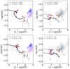 |
Fig. 5. Effects of including rotational yields from PISN in the early evolution of the Fe/O (left panels) and N/O (right panels) as a function of the metallicity 12+log(O/H). The upper panels refer to Zcr = 0.0001, the lower panels refer to Zcr = 0.01. Symbols are the same as in Fig. 2. |
The starburst ages derived by Kojima et al. (2021) from spectral synthesis modelling are young for all the galaxies plotted in Fig. 5, with ages ≤100 Myr. This implies that the metallicity in these objects, e.g., 12+log(O/H), must grow very quickly, possibly requiring a top-heavy IMF. Thus, comparing the left panels of Figs. 5 and 2, we clearly see that an early burst of VMOs is needed to reproduce the observed high values of the Fe/O ratio and of the 12+log(O/H), at early times. For the N/O ratio, these conditions are not nearly enough. Looking at the right panels of the figure, we see that rotation is indeed an essential ingredient to reproduce nitrogen enrichment at very low metallicity.
We note that, while Fe yields are only mildly affected by rotation, N yields do strongly depend on it (Limongi & Chieffi 2018). We remind the reader that this conclusion for the Fe yields by PISNe is mainly based on the results obtained by Takahashi et al. (2018) who computed both the pre-SN evolution and the following explosive models for models with and without rotation (e.g., Fig. 1). For N, we know that only the pre-SN evolution conditions matter and that other parameters beside rotation may affect its yields, in particular that describing the envelope overshooting (Costa et al. 2021). In order to reproduce the observed N/O ratios of EMPG 3 and EMPG 10, we need to use massive star models with an initial rotation parameter between ω = 0.3 (solid lines) and ω = 0.4 (dashed lines).
In all the plots, the solid squares along the models mark ages of 5, 20, 30, 60, 100, and 200 Myr, with the latter being the rightmost point. In the Fe/O diagrams, EMPG 3 and EMPG 10 can be well fitted with both the cases of Zcr = 0.0001 and Zcr = 0.01 and for any rotation value. The timescale of the enrichment indicates, at least for EMPG 10, an age slightly higher than 5 Myr, which is compatible with the very young ages derived from spectrophotometry (Kojima et al. 2021). EMPG 3 could also be compatible even with a lower Fe/O ratio, but in this case the age would be older yet still in the observed range.
In the case of Zcr = 0.0001, the N/O ratio of EMPG 10 is marginally fitted with the higher rotation young model. For EMPG 3 we only have an upper limit on the N/O ratio and model M4ω4 fits its position very well in both diagrams. However, this model requires two quite different ages for Fe/O and N/O, respectively. The best solution for Zcr = 0.0001 is provided by model M4ω3 with an age ≥5 Myr.
By relaxing the critical metallicity to Zcr = 0.01, more solutions are possible. EMPG 10 can be well fitted by the M5ω4 model at an age ≥5 Myr or even at an age = 20 Myr. On the other hand, for EMPG 3 the best model is again the M5ω3 for an age ≥5 Myr or even at an age of =20 Myr.
In any case, the presence of an initial burst of VMOs can explain the data, as assumed in models M4ω3, M4ω4, M5ω3, and M5ω4. These models show also another interesting feature, which is their rapid Fe/O decline at increasing 12+log(O/H) , as a consequence of the suppression of the VMO burst, when the critical metallicity is reached. This feature is also visible in model M3 (Fig. 2), but in this case, as discussed above, the threshold metallicity (Zcrse) for the suppression of the PISN channel depends on stellar evolution, when large mass-loss rates are boosted by a high metallicity. In our models and for an MUP = 350 M⊙, Zcrse ∼ 0.4 (Goswami et al. 2021).
The metal-poor galaxies analysed by Kojima et al. (2021) actually show a trend of declining Fe/O at increasing 12+log(O/H), as shown in Fig. 5. However, this trend cannot be explained by the models presented in that figure if, together with the abundances, we consider that the observed galaxies are all dominated by active starbursts with ages below 50 Myr. The oldest of our models already has an age of 200 Myr and marginally reaches the bulk of the remaining metal-poor galaxies in the Fe/O diagram, while it cannot reach them in the N/O diagram. We note, however, that many of them show Fe/O and N/O ratios that are even below those observed among the bulk of low-metallicity stars. While low values of N/O are expected among non-rotating models, the low Fe/O ratios could also challenge standard chemical evolution models, as may be seen in Fig. 2.
However, the relatively low Fe/O ratio of ‘evolved’ young metal-poor starburst galaxies could be explained by a combination of an early burst of VMO, as for EMPG 3 and EMPG 10, and a population of stars that produces the oxygen-rich/iron-poor ejecta. This could have the twofold effect of favouring a fast 12+log(O/H) evolution and, at the same time, a rapid decline of the Fe/O ratio. Such a model can be obtained by combining an early burst of VMO stars, as in the case of models M4ω3, M4ω4, M5ω3, M5ω4, and a model that includes a top-heavy IMF with MUP ≤ 200 M⊙. For the VMO component, we adopted the same form of the M4ω3 IMF and, when Zcr = 0.0001 is reached and the IMF turns into a standard Kroupa-like one, the formation of a small fraction of low-mass VMOs (Mi≤ 150 M⊙) is still allowed, with an exponent xUP = 0.9. Furthermore, in order to comply with the fast enrichment required by the age estimates performed by Kojima et al. (2021), we need to use a relatively high star formation rate efficiency ν = 5. The properties of the considered models, M6ω3 and M6ω4, are given in Table 2.
The evolution of the Fe/O and N/O ratios obtained with these models is shown in Fig. 6. Their metallicity 12+log(O/H) rises rapidly up to the value corresponding to Zcr = 0.0001. Beyond this point, the Fe/O ratios, which initially correspond to those of EMPG 10, begin a rapid decrease, reaching the value observed in EMPG 6. Later, at an age between 20 and 60 Myr, both models reach the position occupied by the other EMPRESS galaxies. Only EMPG 5 cannot be reproduced by these models. However, we remind the reader that, at the higher metallicities, the estimate of the Fe/O ratios is generally more uncertain because of selective dust depletion (Rodríguez & Rubin 2005; Izotov et al. 2006). As far as the N/O ratio is concerned, only model M6ω4 is able to fit the observations, while model M6ω3 has a too low N/O ratio.
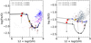 |
Fig. 6. Fe/O (left panel) and N/O (right panel) in models M6ω3 (solid lines) and M6ω4 (dashed lines) as a function of the metallicity 12+log(O/H). The panels refer to Zcr = 0.0001 and the symbols are the same as in Fig. 2. |
6. Conclusions
In this work, we analysed the recent observations of EMPGs galaxies with peculiarly high Fe/O and young starburst ages (Kojima et al. 2021). We initially investigated these peculiarities using the recent yields from Goswami et al. (2021), which take into account the later evolutionary stages of non-rotating massive stars, such as PISN and PPISN. We ran different chemical evolution models with different IMF upper mass limits and slopes. We have shown that, in order to reproduce the high Fe/O ratios observed at 12+log(O/H) ∼ 7 in EMPG 3 and, in particular, in EMPG 10, we need to include the effects of PISN, as in model M3. Other solutions are excluded because the early evolution of such starbursts keeps information of the ejecta of the most massive stars, and only PISN coming from a VMO distribution that produces the right He core masses is able to produce the right ejecta. However, we also show that in order to reproduce the observed primary N behaviour of these EMPGs, we need to consider stars with suitable rotation. For model M3, with a top-heavy IMF up to 300 M⊙ and xUP = 0.6, while it reaches a large Fe/O ratio, on one side it is not able to reach that of EMPG 10 and, on the other, it shows a too low N/O ratio that decreases even more with an increasing contribution of non-rotating PISNs.
We thus complemented yields from Goswami et al. (2021) with new very massive star models with different initial rotational velocities, from ω = 0.1 to ω = 0.6. In rotating massive stars nitrogen is a product of pre-supernova evolution that is barely changed by the final explosion. Our calculations show that N production from the PISN depends very strongly on the initial degree of rotation. While without rotation the N contribution is negligible, it becomes stronger at increasing rotational velocities (see also Takahashi et al. 2018).
Furthermore, to properly account for PISN in the chemical evolution code, we adopted a bi-modal IMF. During the early evolution, the IMF is skewed towards VMOs following the prescriptions of Wise et al. (2012, see Eq. (4)). Since, according to existing theoretical investigations, VMOs producing PISN may form only in very metal-poor environments, with Z/Z⊙ ≤ Zcr, we also assume that when the metallicity encompasses Zcr, the IMF changes to a standard Kroupa IMF (Eq. (3)). We considered two values of the critical metallicity, Zcr = 0.0001 and Zcr = 0.01, corresponding to efficient and inefficient dust cooling, respectively (Salvadori et al. 2008; Schneider et al. 2006).
With such a bi-modal IMF and a yield family for different rotational velocities, we searched for suitable chemical evolution models that could explain the main characteristics of EMPG 3 and EMPG 10 namely, (i) relatively high 12+log(O/H) at very young ages, (ii) high Fe/O ratios and (iii) ‘standard’, i.e., typical of low metallicity stars, N/O ratios. The first point requires a rapid and efficient enrichment. We adopted short star formation and infall timescales, ν = 1 Gyr−1 and tinf = 0.1 Gyr, respectively. The second point can be obtained only by means of a suitable population of PISN for which we adopted the IMF of Eq. (4) with Mchar = 200 M⊙. Other values of Mchar between 200 M⊙ and 300 M⊙ produce almost the same results, while for Mchar < 200 M⊙ the Fe production is too low. The third point requires models with rotation. We find that, with initial rotation parameters of ω = 0.3 and ω = 0.4, we could bracket the observed N/O ratios of EMPG 3 and EMPG 10, as shown in Fig. 5. Though the threshold metallicity with Zcr = 0.0001 is very low, our models M4ω3 and M4ω4 are able to fit both EMPG galaxies at the observed metallicity, 12+log(O/H), and at young ages. When Zcr is reached, the number of VMOs formed after normalisation with respect to the observed masses of EMPG 3 and EMPG 10 is 194 and 394, respectively. Considering the relative evolutionary timescales, these stars should explode at an average rate of one per 20 000 yr and one per 7000 yr in EMPG 3 and EMPG 10, respectively.
A common feature of the EMPRESS galaxies is that they are dominated by very young starbursts with high specific star formation rates. Contrary to EMPG 3 and EMPG 10, most of them are characterised by a low Fe/O ratio, which is generally near or even below the lower envelope of the stellar data. Models M1, M2, and M3 cannot reproduce these peculiarities. This is also true for models with rotation, as can be seen in Fig. 5. Nevertheless, their low Fe/O could be indicative of an excess of oxygen produced by the less massive PISN, as can be inferred from Fig. 1. We have thus researched whether some variants of models M4 and M5 could provide a viable explanation. In order to comply with the young ages observed, we performed a few tests by increasing the star formation efficiency to ν = 5 Gyr−1. This is not enough, however. The only galaxy that could be explained is EMPG 6, which has an Fe/O value well within the range observed in metal-poor stars. Instead, if we allow the secondary Kroupa IMF to extend up to MUP = 150 M⊙ with xUP = 0.9, i.e., a top-heavy Kroupa IMF, we obtain a model (M6ω4) that can also match the positions of the other EMPRESS starbursts at relatively young ages, in both the Fe/O and N/O vs. 12+log(O/H) diagrams, as shown in Fig. 6.
We recall that an IMF favouring the formation of massive stars in regimes of bursting star formation has already been claimed in the past (Marks et al. 2012; Jeřábková et al. 2018; Zhang et al. 2018). Moreover, we have already shown that there is strong evidence of a well-populated IMF up to MUP = 200 M⊙ in 30 Doradus, with an estimated xUP ∼ 0.9 (Crowther et al. 2010; Schneider et al. 2018a). In summary, several peculiarities observed among very metal-poor starbursts could be explained within a single scenario, in which a high specific SFR produces a fast self-enrichment that drives them first into a phase of high Fe production, and then quickly into the phase of high O production. Thus, if PISN arise only in high specific SFR objects, this fast evolution could challenge their detection in the local Universe.
In this respect, we note that the imprinting left by very massive stars, not only in terms of chemical composition (Takahashi et al. 2018) but also of chemical evolutionary timescales, could be another important signature to establish the nature of the upper tail of the IMF and its deviations from universality (Elmegreen & Shadmehri 2003; Kroupa 2008; Marks et al. 2012; Hosek et al. 2019; Romano et al. 2020). Finally, we recall that recent gravitational wave detection (Abbott et al. 2016, 2020) has drawn attention to a large variety of phenomena that could affect the estimation of the initial masses and metallicities of PISN progenitors and their yields, arising from current uncertainties in single stellar-evolution theory (e.g., Costa et al. 2021), possible effects of rotation (e.g., Takahashi et al. 2018), and also binary interaction (e.g., Han et al. 2020; Spera et al. 2019; Stanway & Eldridge 2018; Hurley et al. 2002). In summary, a variation of the mass and metallicity domain from where PISN might arise will immediately impact the choice of the IMF parameters needed to reproduce EMPG observations. On the contrary, the study of these galaxies could have a great impact on our understanding of the uncertainties still affecting stellar-evolution models.
Acknowledgments
We thank the anonymous referee for her/his useful suggestions. This work has been partially supported by PRIN MIUR 2017 prot. 20173ML3WW 001 and 002, ‘Opening the ALMA window on the cosmic evolution of gas, stars and supermassive black holes’. S.G. acknowledges support from Project CRISP PTDC/FIS-AST-31546/2017 funded by FCT. G.C. acknowledges financial support from the European Research Council for the ERC Consolidator grant DEMOBLACK, under contract no. 770017. P.M. acknowledges support from the project PRD 2021 (University of Padova). M.S. acknowledges funding from the European Union’s Horizon 2020 research and innovation programme under the Marie-Skłodowska-Curie grant agreement No. 794393.
References
- Abbott, B. P., Abbott, R., Abbott, T. D., et al. 2016, Phys. Rev. Lett., 116, 061102 [Google Scholar]
- Abbott, R., Abbott, T. D., Abraham, S., et al. 2020, Phys. Rev. Lett., 125, 101102 [Google Scholar]
- Aihara, H., Arimoto, N., Armstrong, R., et al. 2018, PASJ, 70, S4 [NASA ADS] [Google Scholar]
- Asplund, M., Grevesse, N., Sauval, A. J., & Scott, P. 2009, ARA&A, 47, 481 [NASA ADS] [CrossRef] [Google Scholar]
- Bensby, T., Feltzing, S., & Oey, M. S. 2014, A&A, 562, A71 [NASA ADS] [CrossRef] [EDP Sciences] [Google Scholar]
- Bressan, A., Marigo, P., Girardi, L., et al. 2012, MNRAS, 427, 127 [NASA ADS] [CrossRef] [Google Scholar]
- Cayrel, R., Depagne, E., Spite, M., et al. 2004, A&A, 416, 1117 [NASA ADS] [CrossRef] [EDP Sciences] [Google Scholar]
- Chabrier, G. 2003, PASP, 115, 763 [Google Scholar]
- Chen, K.-J., Woosley, S., Heger, A., Almgren, A., & Whalen, D. J. 2014, ApJ, 792, 28 [NASA ADS] [CrossRef] [Google Scholar]
- Chieffi, A., & Limongi, M. 2004, ApJ, 608, 405 [NASA ADS] [CrossRef] [Google Scholar]
- Christensen, L., Laursen, P., Richard, J., et al. 2012a, MNRAS, 427, 1973 [NASA ADS] [CrossRef] [Google Scholar]
- Christensen, L., Richard, J., Hjorth, J., et al. 2012b, MNRAS, 427, 1953 [Google Scholar]
- Costa, G., Girardi, L., Bressan, A., et al. 2019, MNRAS, 485, 4641 [NASA ADS] [CrossRef] [Google Scholar]
- Costa, G., Bressan, A., Mapelli, M., et al. 2021, MNRAS, 501, 4514 [NASA ADS] [CrossRef] [Google Scholar]
- Crowther, P. A., Schnurr, O., Hirschi, R., et al. 2010, MNRAS, 408, 731 [Google Scholar]
- Crowther, P. A., Caballero-Nieves, S. M., Bostroem, K. A., et al. 2016, MNRAS, 458, 624 [Google Scholar]
- Elmegreen, B. G., & Shadmehri, M. 2003, MNRAS, 338, 817 [NASA ADS] [CrossRef] [Google Scholar]
- Fontanot, F., Somerville, R. S., Silva, L., Monaco, P., & Skibba, R. 2009, MNRAS, 392, 553 [NASA ADS] [CrossRef] [Google Scholar]
- Fujita, A., Mac Low, M.-M., Ferrara, A., & Meiksin, A. 2004, ApJ, 613, 159 [NASA ADS] [CrossRef] [Google Scholar]
- Goswami, A., & Prantzos, N. 2000, A&A, 359, 191 [NASA ADS] [Google Scholar]
- Goswami, S., Slemer, A., Marigo, P., et al. 2021, A&A, 650, A203 [NASA ADS] [CrossRef] [EDP Sciences] [Google Scholar]
- Grisoni, V., Spitoni, E., Matteucci, F., et al. 2017, MNRAS, 472, 3637 [Google Scholar]
- Grisoni, V., Spitoni, E., & Matteucci, F. 2018, MNRAS, 481, 2570 [NASA ADS] [Google Scholar]
- Grisoni, V., Matteucci, F., Romano, D., & Fu, X. 2019, MNRAS, 489, 3539 [NASA ADS] [CrossRef] [Google Scholar]
- Grisoni, V., Cescutti, G., Matteucci, F., et al. 2020a, MNRAS, 492, 2828 [Google Scholar]
- Grisoni, V., Romano, D., Spitoni, E., et al. 2020b, MNRAS, 498, 1252 [NASA ADS] [CrossRef] [Google Scholar]
- Grisoni, V., Matteucci, F., & Romano, D. 2021, MNRAS, 508, 719 [NASA ADS] [CrossRef] [Google Scholar]
- Han, Z.-W., Ge, H.-W., Chen, X.-F., & Chen, H.-L. 2020, Res. Astron. Astrophys., 20, 161 [CrossRef] [Google Scholar]
- Heger, A., & Woosley, S. E. 2002, ApJ, 567, 532 [Google Scholar]
- Heger, A., Fryer, C. L., Woosley, S. E., Langer, N., & Hartmann, D. H. 2003, ApJ, 591, 288 [CrossRef] [Google Scholar]
- Hirschauer, A. S., Salzer, J. J., Skillman, E. D., et al. 2016, ApJ, 822, 108 [NASA ADS] [CrossRef] [Google Scholar]
- Hosek, M. W., Jr, Lu, J. R., Anderson, J., et al. 2019, ApJ, 870, 44 [Google Scholar]
- Hsyu, T., Cooke, R. J., Prochaska, J. X., & Bolte, M. 2017, ApJ, 845, L22 [NASA ADS] [CrossRef] [Google Scholar]
- Hunt, L. K., De Looze, I., Boquien, M., et al. 2019, A&A, 621, A51 [NASA ADS] [CrossRef] [EDP Sciences] [Google Scholar]
- Hurley, J. R., Tout, C. A., & Pols, O. R. 2002, MNRAS, 329, 897 [Google Scholar]
- Isobe, Y., Ouchi, M., Kojima, T., et al. 2021, ApJ, 918, 54 [NASA ADS] [CrossRef] [Google Scholar]
- Isobe, Y., Ouchi, M., Suzuki, A., et al. 2022, ApJ, 925, 111 [NASA ADS] [CrossRef] [Google Scholar]
- Iwamoto, K., Brachwitz, F., Nomoto, K., et al. 1999, ApJS, 125, 439 [NASA ADS] [CrossRef] [Google Scholar]
- Izotov, Y. I., & Thuan, T. X. 1998, ApJ, 500, 188 [NASA ADS] [CrossRef] [Google Scholar]
- Izotov, Y. I., Stasińska, G., Meynet, G., Guseva, N. G., & Thuan, T. X. 2006, A&A, 448, 955 [CrossRef] [EDP Sciences] [Google Scholar]
- Izotov, Y. I., Guseva, N. G., Fricke, K. J., & Papaderos, P. 2009, A&A, 503, 61 [NASA ADS] [CrossRef] [EDP Sciences] [Google Scholar]
- Izotov, Y. I., Thuan, T. X., & Guseva, N. G. 2012, A&A, 546, A122 [NASA ADS] [CrossRef] [EDP Sciences] [Google Scholar]
- Izotov, Y. I., Thuan, T. X., Guseva, N. G., & Liss, S. E. 2018, MNRAS, 473, 1956 [NASA ADS] [CrossRef] [Google Scholar]
- Izotov, Y. I., Thuan, T. X., & Guseva, N. G. 2019, MNRAS, 483, 5491 [NASA ADS] [CrossRef] [Google Scholar]
- Jeřábková, T., Hasani Zonoozi, A., Kroupa, P., et al. 2018, A&A, 620, A39 [Google Scholar]
- Kennicutt, R. C., Jr. 1998, ApJ, 498, 541 [Google Scholar]
- Kojima, T., Ouchi, M., Rauch, M., et al. 2020, ApJ, 898, 142 [NASA ADS] [CrossRef] [Google Scholar]
- Kojima, T., Ouchi, M., Rauch, M., et al. 2021, ApJ, 913, 22 [NASA ADS] [CrossRef] [Google Scholar]
- Kozyreva, A., Yoon, S.-C., & Langer, N. 2014, A&A, 566, A146 [NASA ADS] [CrossRef] [EDP Sciences] [Google Scholar]
- Kroupa, P. 2008, in Pathways Through an Eclectic Universe, eds. J. H. Knapen, T. J. Mahoney, & A. Vazdekis, ASP Conf. Ser., 390, 3 [Google Scholar]
- Kroupa, P., Tout, C. A., & Gilmore, G. 1993, MNRAS, 262, 545 [NASA ADS] [CrossRef] [Google Scholar]
- Kunth, D., & Östlin, G. 2000, A&ARv, 10, 1 [NASA ADS] [CrossRef] [Google Scholar]
- Langer, N. 2012, ARA&A, 50, 107 [CrossRef] [Google Scholar]
- Limongi, M., & Chieffi, A. 2018, VizieR Online Data Catalog: J/ApJS/237/13 [Google Scholar]
- Lo Faro, B., Franceschini, A., Vaccari, M., et al. 2013, ApJ, 762, 108 [NASA ADS] [CrossRef] [Google Scholar]
- Lo Faro, B., Silva, L., Franceschini, A., Miller, N., & Efstathiou, A. 2015, MNRAS, 447, 3442 [NASA ADS] [CrossRef] [Google Scholar]
- Mac Low, M.-M., & Ferrara, A. 1999, ApJ, 513, 142 [NASA ADS] [CrossRef] [Google Scholar]
- Mainali, R., Kollmeier, J. A., Stark, D. P., et al. 2017, ApJ, 836, L14 [Google Scholar]
- Marconi, G., Matteucci, F., & Tosi, M. 1994, MNRAS, 270, 35 [NASA ADS] [CrossRef] [Google Scholar]
- Marigo, P., Cummings, J. D., Curtis, J. L., et al. 2020, Nat. Astron., 4, 1102 [NASA ADS] [CrossRef] [Google Scholar]
- Marks, M., Kroupa, P., Dabringhausen, J., & Pawlowski, M. S. 2012, MNRAS, 422, 2246 [NASA ADS] [CrossRef] [Google Scholar]
- Matteucci, F. 2021, A&ARv, 29, 5 [NASA ADS] [CrossRef] [Google Scholar]
- Matteucci, F., & Greggio, L. 1986, A&A, 154, 279 [NASA ADS] [Google Scholar]
- Miyazaki, S., Komiyama, Y., Kawanomoto, S., et al. 2018, PASJ, 70, S1 [NASA ADS] [Google Scholar]
- Ohkubo, T., Umeda, H., Maeda, K., et al. 2006, ApJ, 645, 1352 [NASA ADS] [CrossRef] [Google Scholar]
- Ott, J., Walter, F., & Brinks, E. 2005, MNRAS, 358, 1453 [NASA ADS] [CrossRef] [Google Scholar]
- Pettini, M., Ellison, S. L., Bergeron, J., & Petitjean, P. 2002, A&A, 391, 21 [NASA ADS] [CrossRef] [EDP Sciences] [Google Scholar]
- Pettini, M., Zych, B. J., Steidel, C. C., & Chaffee, F. H. 2008, MNRAS, 385, 2011 [NASA ADS] [CrossRef] [Google Scholar]
- Pilyugin, L. S. 1993, A&A, 277, 42 [NASA ADS] [Google Scholar]
- Prantzos, N., Abia, C., Limongi, M., Chieffi, A., & Cristallo, S. 2018, MNRAS, 476, 3432 [Google Scholar]
- Pustilnik, S. A., Kniazev, A. Y., & Pramskij, A. G. 2005, A&A, 443, 91 [NASA ADS] [CrossRef] [EDP Sciences] [Google Scholar]
- Recchi, S., & Hensler, G. 2007, A&A, 476, 841 [NASA ADS] [CrossRef] [EDP Sciences] [Google Scholar]
- Recchi, S., Matteucci, F., & D’Ercole, A. 2001, MNRAS, 322, 800 [NASA ADS] [CrossRef] [Google Scholar]
- Recchi, S., Matteucci, F., D’Ercole, A., & Tosi, M. 2004, A&A, 426, 37 [NASA ADS] [CrossRef] [EDP Sciences] [Google Scholar]
- Recchi, S., Spitoni, E., Matteucci, F., & Lanfranchi, G. A. 2008, A&A, 489, 555 [NASA ADS] [CrossRef] [EDP Sciences] [Google Scholar]
- Ritter, C., Herwig, F., Jones, S., et al. 2018, MNRAS, 480, 538 [NASA ADS] [CrossRef] [Google Scholar]
- Rodríguez, M., & Rubin, R. H. 2005, ApJ, 626, 900 [CrossRef] [Google Scholar]
- Romano, D., Franchini, M., Grisoni, V., et al. 2020, A&A, 639, A37 [NASA ADS] [CrossRef] [EDP Sciences] [Google Scholar]
- Salvadori, S., Ferrara, A., & Schneider, R. 2008, MNRAS, 386, 348 [Google Scholar]
- Salvadori, S., Tolstoy, E., Ferrara, A., & Zaroubi, S. 2014, MNRAS, 437, L26 [NASA ADS] [CrossRef] [Google Scholar]
- Salvadori, S., Bonifacio, P., Caffau, E., et al. 2019, MNRAS, 487, 4261 [NASA ADS] [CrossRef] [Google Scholar]
- Schneider, R., Ferrara, A., Natarajan, P., & Omukai, K. 2002, ApJ, 571, 30 [CrossRef] [Google Scholar]
- Schneider, R., Omukai, K., Inoue, A. K., & Ferrara, A. 2006, MNRAS, 369, 1437 [NASA ADS] [CrossRef] [Google Scholar]
- Schneider, F. R. N., Sana, H., Evans, C. J., et al. 2018a, Science, 359, 69 [NASA ADS] [CrossRef] [Google Scholar]
- Schneider, F. R. N., Ramírez-Agudelo, O. H., Tramper, F., et al. 2018b, A&A, 618, A73 [NASA ADS] [CrossRef] [EDP Sciences] [Google Scholar]
- Silva, L., Granato, G. L., Bressan, A., & Danese, L. 1998, ApJ, 509, 103 [Google Scholar]
- Silva, L., Schurer, A., Granato, G. L., et al. 2011, MNRAS, 410, 2043 [NASA ADS] [Google Scholar]
- Skillman, E. D., Salzer, J. J., Berg, D. A., et al. 2013, AJ, 146, 3 [CrossRef] [Google Scholar]
- Spera, M., Mapelli, M., Giacobbo, N., et al. 2019, MNRAS, 485, 889 [Google Scholar]
- Spitoni, E., Verma, K., Silva Aguirre, V., et al. 2021, A&A, 647, A73 [EDP Sciences] [Google Scholar]
- Stanway, E. R., & Eldridge, J. J. 2018, MNRAS, 479, 75–93 [NASA ADS] [CrossRef] [Google Scholar]
- Stark, D. P., Ellis, R. S., Charlot, S., et al. 2017, MNRAS, 464, 469 [NASA ADS] [CrossRef] [Google Scholar]
- Takahashi, K., Yoshida, T., & Umeda, H. 2018, ApJ, 857, 111 [NASA ADS] [CrossRef] [Google Scholar]
- Thuan, T. X., & Izotov, Y. I. 2005, ApJS, 161, 240 [NASA ADS] [CrossRef] [Google Scholar]
- Vanzella, E., Calura, F., Meneghetti, M., et al. 2017, MNRAS, 467, 4304 [Google Scholar]
- Vega, O., Clemens, M. S., Bressan, A., et al. 2008, A&A, 484, 631 [NASA ADS] [CrossRef] [EDP Sciences] [Google Scholar]
- Wanajo, S., Nomoto, K., Janka, H. T., Kitaura, F. S., & Müller, B. 2009, ApJ, 695, 208 [NASA ADS] [CrossRef] [Google Scholar]
- Wise, J. H., Abel, T., Turk, M. J., Norman, M. L., & Smith, B. D. 2012, MNRAS, 427, 311 [NASA ADS] [CrossRef] [Google Scholar]
- Woosley, S. E. 2017, ApJ, 836, 244 [Google Scholar]
- Woosley, S. E., Heger, A., & Weaver, T. A. 2002, Rev. Mod. Phys., 74, 1015 [NASA ADS] [CrossRef] [Google Scholar]
- Yoshida, T., Umeda, H., Maeda, K., & Ishii, T. 2016, MNRAS, 457, 351 [Google Scholar]
- Zhang, Z.-Y., Romano, D., Ivison, R. J., Papadopoulos, P. P., & Matteucci, F. 2018, Nature, 558, 260 [Google Scholar]
All Tables
Input parameters of selected chemical evolution and yield models. MTW is our set of stellar ejecta described in Goswami et al. (2021).
Chemical evolution model parameters and properties of the initial VMO burst when the gas metallicity reaches Z = Zcr.
All Figures
|
Fig. 1. C12, N14, O16, and Fe PISN yields from Z = 0.0001 rotational models of this work (green, solid, and dotted lines for 2 rotation rate values) based on pure He non-rotating models (blue) from Heger & Woosley (2002). In red, we show rotating (solid) and non-rotating (dotted) yields by Takahashi et al. (2018). We note that N14 yields from non-rotating models are negligible. |
| In the text | |
|
Fig. 2. Fe/O ratio (left panel) and N/O ratio (right panel) as a function of the metallicity, 12+log(O/H). EMPGs from Kojima et al. (2021) are shown as numbered circles from 1 to 9. Object 10 is the EMPG from Izotov et al. (2018). The lowest metallicity EMPGs are are highlighted as filled circles (red for objects 3 and 10, and orange for the intermediate object 6). In the left panel, blue and magenta dots represent, respectively, thin and thick disc stars from Bensby et al. (2014), and grey dots represent low-metallicity stars from Cayrel et al. (2004). In the right panel, light grey dots correspond to local galaxies from Izotov et al. (2006), and dark grey dots are assembled from Pettini et al. (2002) and Pettini et al. (2008), which are for extragalactic H II regions and high-redshift DLA systems. Solid line with squares show the evolution of the abundance ratios for the models of Table 1. The six squares mark, from left to right, model ages at 5, 20, 30 , 60, 100, and 200 Myr, respectively, the latter being larger than the estimated upper limit by Kojima et al. (2021). See text for details. |
| In the text | |
|
Fig. 3. Adopted IMF for chemical evolution of models M4ω4 (solid red line) and M5ω4 (dot-dashed red line). The VMO IMF distributions are given by Eq. (4) with Mchar = 200 M⊙ and normalised to the cumulative mass reached at the corresponding Zcr. For comparison, the IMFs of the post-VMO burst phases, with the same mass normalisation, are also shown (black lines). The expected number of VMOs is shown in the label and in Table 2. |
| In the text | |
|
Fig. 4. Evolution of gas metallicity (solid lines) and cumulative mass converted into stars (dash-dotted lines) of models that include an early burst of VMOs exploding as PISN. The threshold metallicity for VMO formation is Zcr = 10−4 (M4ω4, upper panel) and 10−2 (M5ω4, lower panel). Their IMF distribution is shown in Fig. 3. In both panels the adopted Mchar is 200 M⊙. See text for details. |
| In the text | |
|
Fig. 5. Effects of including rotational yields from PISN in the early evolution of the Fe/O (left panels) and N/O (right panels) as a function of the metallicity 12+log(O/H). The upper panels refer to Zcr = 0.0001, the lower panels refer to Zcr = 0.01. Symbols are the same as in Fig. 2. |
| In the text | |
|
Fig. 6. Fe/O (left panel) and N/O (right panel) in models M6ω3 (solid lines) and M6ω4 (dashed lines) as a function of the metallicity 12+log(O/H). The panels refer to Zcr = 0.0001 and the symbols are the same as in Fig. 2. |
| In the text | |
Current usage metrics show cumulative count of Article Views (full-text article views including HTML views, PDF and ePub downloads, according to the available data) and Abstracts Views on Vision4Press platform.
Data correspond to usage on the plateform after 2015. The current usage metrics is available 48-96 hours after online publication and is updated daily on week days.
Initial download of the metrics may take a while.