| Issue |
A&A
Volume 662, June 2022
|
|
|---|---|---|
| Article Number | A75 | |
| Number of page(s) | 16 | |
| Section | Extragalactic astronomy | |
| DOI | https://doi.org/10.1051/0004-6361/202142597 | |
| Published online | 17 June 2022 | |
Ca II triplet spectroscopy of Small Magellanic Cloud red giants
V. Abundances and velocities for 12 massive clusters⋆
1
Observatorio Astronómico, Universidad Nacional de Córdoba, Laprida 854, X5000BGR Córdoba, Argentina
e-mail: This email address is being protected from spambots. You need JavaScript enabled to view it.
2
Instituto de Astronomía Teórica y Experimental (CONICET-UNC), Laprida 854, X5000BGR Córdoba, Argentina
3
Consejo Nacional de Investigaciones Científicas y Técnicas (CONICET), Godoy Cruz 2290, Buenos Aires CPC 1425FQB, Argentina
4
Departamento de Astronomía, Casilla 160-C, Universidad de Concepción, Concepción, Chile
5
Instituto de Investigación Multidisciplinario en Ciencia y Tecnología, Universidad de La Serena. Avenida Raúl Bitrán S/N, La Serena, Chile
6
Departamento de Astronomía, Facultad de Ciencias, Universidad de La Serena, Av. Juan Cisternas 1200, La Serena, Chile
7
Instituto de Alta Investigación, Universidad de Tarapacá, Casilla 7D, Arica, Chile
8
Research School of Astronomy and Astrophysics, Australian National University, Canberra, ACT 2611, Australia
9
Astronomisches Rechen-Institut, Zentrum für Astronomie der Universität Heidelberg, Mönchhofstr. 12-14, 69120 Heidelberg, Germany
Received:
5
November
2021
Accepted:
11
March
2022
Abstract
Aims. We aim to analyze the chemical evolution of the Small Magellanic Cloud, adding 12 additional clusters to our existing sample, based on accurate and homogeneously derived metallicities. We are particularly interested in seeing if there is any correlation between age and metallicity for the different structural components to which the clusters belong, taking into account their positions relative to the different tidal structures present in the galaxy.
Methods. The spectroscopic metallicities of red giant stars were derived from the measurement of the equivalent width of the near-IR calcium triplet lines. Our cluster membership analysis was carried out using criteria that include radial velocities, metallicities, proper motions, and distances from the cluster center.
Results. The mean cluster radial velocity and metallicity were determined with a typical error of 2.1 km s−1 and 0.03 dex, respectively. We added this information to that available in the literature for other clusters studied with the same method, compiling a final sample of 48 clusters with metallicities that were homogeneously determined. The clusters of the final sample are distributed across an area of ∼70 deg2 and cover an age range from 0.4 Gyr to 10.5 Gyr. This is the largest sample of spectroscopically analyzed SMC clusters available to date.
Conclusions. We confirm the large cluster metallicity dispersion (∼0.6 dex) at any given age in the inner region of the SMC. The metallicity distribution of our new cluster sample shows a lower probability of being bimodal than suggested in previous studies. The separate chemical analysis of clusters in the six components (Main Body, Counter-Bridge, West Halo, Wing/Bridge, Northern Bridge, and Southern Bridge) shows that only clusters belonging to the Northern Bridge appear to trace a V-Shape, showing a clear inversion of the metallicity gradient in the outer regions. There is a suggestion of a metallicity gradient in the West Halo, similar to that previously found for field stars. It presents, however, a very broad uncertainty. Also, clusters belonging to the West Halo, Wing/Bridge, and Southern Bridge exhibit a well-defined age-metallicity relation with relatively little scatter in terms of abundance at a fixed age compared to other regions.
Key words: galaxies: star clusters: general / Magellanic Clouds / stars: abundances
Full Table 2 is only available at the CDS via anonymous ftp to cdsarc.u-strasbg.fr (130.79.128.5) or via http://cdsarc.u-strasbg.fr/viz-bin/cat/J/A+A/662/A75
© ESO 2022
1. Introduction
The Magellanic Clouds (MCs) constitute the pair of interacting galaxies closest to the Milky Way (MW). They consist of the Large Magellanic Cloud (LMC) and the Small Magellanic Cloud (SMC), located at distances of ∼49.59 ± 0.09 kpc (Pietrzyński et al. 2019) and 62.44 ± 0.47 kpc (Graczyk et al. 2020) from the MW, respectively. The MCs are embedded within a diffuse structure of HI gas, where different components can be identified, such as the Magellanic Stream and the Leading Arm (Mathewson et al. 1974; Putman et al. 2003; Nidever et al. 2008, 2010; D’Onghia & Fox 2016). These features have been interpreted as a consequence of the LMC-SMC interactions or the interaction of the two galaxies with the MW (Besla et al. 2010, 2012; Diaz & Bekki 2011, 2012). For a long time it was thought that the MCs had orbited the MW multiple times (Kallivayalil et al. 2006a,b). However, more recent works have strongly suggested that both galaxies are experiencing their first close encounter with our Galaxy (Besla et al. 2007; Piatek et al. 2008; Kallivayalil et al. 2013; Gaia Collaboration 2016; Patel et al. 2017), based on the latest accurate measurements of proper motions with the Hubble Space Telescope (HST) and Gaia.
Several authors found evidence that the stellar populations of the SMC have been subject to substantial perturbations by forces associated with the LMC (e.g., Evans & Howarth 2008; Haschke et al. 2012a; Dobbie et al. 2014a; Subramanian et al. 2017; De Leo et al. 2020) and reveal complex patterns of velocities consistent with the idea of the SMC being in the process of tidal disruption (e.g., Niederhofer et al. 2018, 2021; Zivick et al. 2018). In addition, stellar tidal tails have been found around both MCs (Besla et al. 2016; Belokurov et al. 2017; Pieres et al. 2017; Mackey et al. 2018; Belokurov & Erkal 2019; Nidever et al. 2019; Gaia Collaboration 2021; El Youssoufi et al. 2021).
Close encounters between gas-rich galaxies will produce enhancement of star formation (e.g., Whitmore et al. 1999) and subsequent chemical enrichment (e.g., Da Costa 1991; Dopita et al. 1997; Pagel & Tautvaisiene 1998). These processes alter, for example, the age and spatial distributions of the stellar populations (Glatt et al. 2010; Nayak et al. 2016, 2018; Bitsakis et al. 2018; Rubele et al. 2018), as well as the metallicity distribution and its gradient (Cioni 2009). In particular, if we want to understand not only the chemical evolution but also other processes like star formation and kinematics in the MCs, it is necessary to have a description of the global dynamics of the Magellanic System, and vice versa: these processes provide important information on parameters related to interactions.
Our group is carrying out a long-term investigation of SMC clusters and field stars using CaII triplet (CaT) spectroscopy (Parisi et al. 2009, 2010, 2015, 2016, hereafter P09, P10, P15, and P16, respectively). As shown by Cole et al. (2004, hereafter C04), the CaT is a very efficient and accurate metallicity indicator, with minimal age effects (Carrera et al. 2013) and independent of the chemical evolution histories (Da Costa 2016).
These investigations have led to several promising results that point to some surprising differences between the clusters and field star population and raise a number of important issues, including: how real the cluster metallicity spread is at a given age and whether it varies with age. If it is real, we want to consider whether it is a global effect or whether it varies with radius or position in the galaxy. Then there is the question of whether the cluster metallicity distribution (MD) is indeed bimodal, the reason clusters and field stars present different MDs, and whether there is such a thing as a cluster metallicity gradient (MG) or not. If so, we consider whether it really ends up inverting in the outer regions. This latter concern, in particular, still remains a very controversial issue. While SMC field stars show an unquestionable MG (P16, Dobbie et al. 2014a; Choudhury et al. 2018, 2020), for the case of the star clusters, the MG is not statistically significant (P15). At the same time, Parisi et al. (2014) did not find a clear age gradient (AG) from a sample of 50 SMC clusters.
On the other hand, Dias et al. (2014, 2016a, hereafter D14 and D16, respectively) introduced the idea that both the AG and the MG, as well as the large dispersion of metallicities that is clearly evident in our AMR (P15), are due to the fact that the complete sample of clusters is analyzed, without taking into account their membership positions in different components of the galaxy carrying potentially different chemodynamic histories. Individual clusters should be studied as part of the respective sky region as these regions may have been created during the perturbed evolution of the SMC. Using the projected distance a (Piatti et al. 2005), D16 suggest that cluster samples should be divided taking into account the tidal morphological characteristics of the SMC. Specifically, D16 divided the catalog of Bica et al. (2008) into four groups depending on whether their positions in the galaxy match the SMC Main Body (a < 2°), the region in which the Wing/Bridge is located, the Counter-Bridge or the West Halo. These last three regions are located in the outer part of the galaxy (a > 2°). They have a clear gas counterpart (Besla 2011) and have been predicted by different models and simulations, as described above.
Since then, more details have been added to this framework. For example, Belokurov et al. (2017) showed that the stellar counterpart of the Magellanic Bridge (Irwin et al. 1985; Omkumar et al. 2021; Dias et al. 2021), widely known to be related to the gaseous bridge containing predominantly younger stars, has a separate southern branch traced by RR Lyrae stars, namely, older stellar populations that are also connecting the SMC to the LMC, although the reality of this feature is in dispute (Jacyszyn-Dobrzeniecka et al. 2020). Dias et al. (2021, hereafter D21) using full phase-space information, revealed that the Magellanic Bridge has a third northern branch with clusters moving towards the LMC, which confirms previous indications by, for instance, Nidever et al. (2017). In D21, the first confirmed star cluster belonging to the tidal counterpart of the Magellanic Bridge was also revealed as the so-called Counter-Bridge (Diaz & Bekki 2012; Muller & Bekki 2007; Ripepi et al. 2017; Muraveva et al. 2018; Omkumar et al. 2021; Dias et al. 2021; Niederhofer et al. 2021). Finally, D16 defined the West Halo, a separate structure that seems to be moving away from the SMC as well. This outward motion was confirmed by proper motions (Zivick et al. 2018; Niederhofer et al. 2018), and Tatton et al. (2021) discussed the possibility that the West Halo is actually the beginning of the Counter-Bridge that appears warped behind the SMC towards the Northeast.
We believe that in order to better help constrain answers to the questions raised above, it is necessary not only to significantly increase the sample of clusters homogeneously studied, but also to analyze the chemical properties of the SMC star cluster system in the context of its dynamical history, namely, to study the clusters recognizing the different present-day environments rather than treating them all together. With this goal in mind, we here add a sample of 12 massive clusters that belong to several different components, studied in exactly the same way as our previous clusters.
In Sect. 2, we describe the observations and the reduction process carried out for the new cluster observations. The measurement of radial velocities and equivalent widths is described in Sect. 3. Section 4 is dedicated to the detailed description of the metallicity determinations. The analysis of the MG and AMR in the SMC is carried out in Sect. 5. Finally, we summarize our conclusions in Sect. 6.
2. Spectroscopic observations and reduction
The observational data used in the present work were downloaded from the ESO Archive1. These observations were carried out in 2005 and 2006 at the VLT at European Southern Observatory (ESO, Paranal, Chile) under the programs 075.B-0548 and 073.B-0488 in service mode (PI: Eva Grebel). The SMC is the only nearby galaxy that has formed and preserved populous star clusters seemingly continuously over the past ∼11 Gyr. Therefore, for this program, populous SMC clusters were selected with prominent red giant branches that sampled and covered the past 11 Gyr, helping to provide a well-sampled AMR and quantifying metallicity spreads at any given age among intermediate-age clusters in the galaxy. The preliminary results of the analysis of these data were presented in Kayser et al. (2007). The selected clusters are listed in Table 1, where we show their different identifications as well as their corresponding equatorial coordinates, the adopted cluster age, mass, and the semimajor axis, a. We adopted the designations of the different SMC components of D16 updated by D21 (shown in Fig. 1) and associate our cluster sample with these components based on the projected line-of-sight locations of our clusters. The resulting associations with the components are listed in the last columns of Table 1.
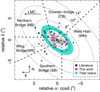 |
Fig. 1. Projected distribution of SMC star clusters from the catalog of Bica et al. (2020) represented by grey dots. Black circles are clusters previously studied with CaT and pink squares clusters studied in this work. Thin dashed lines indicate the ellipses used as a proxy for the distance to the SMC center. The distance a is the semimajor axis of the ellipses indicated in degrees in the figure. The ellipses are tilted by 45° and have an aspect ratio of b/a = 0.5. Thick dashed lines split the regions outside a > 2° into different SMC components. The SMC tidal radius of a = 3.4° |

SMC cluster sample.
In each cluster, spectroscopic targets correspond to red giant stars belonging to the clusters and their surrounding fields. As an example, for the cluster L 38, we show in Figs. 2 and 3 the locations of selected targets in the cluster color-magnitude diagram (CMD) and positional chart. The positions and magnitudes needed to build these figures were obtained from PSF photometry performed on the V and I pre-images taken previously with the same instrument.
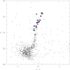 |
Fig. 2. Instrumental color-magnitude diagram of the cluster L 38. The spectroscopic targets are marked with large circles. Blue, cyan, green, and magenta symbols represent stars discarded as cluster members because of their distance from the cluster center, RV, metallicity, and PM values. Red circles show the adopted cluster members. See Sect. 4.2 for details. |
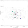 |
Fig. 3. Chart of cluster L 38. Spectroscopic targets are plotted with the same color code as in Fig. 2. The adopted cluster radius is represented by the circle. |
Using the FORS2 instrument on the VLT, the spectra of 502 purported cluster red giant stars were obtained. The instrument, in mask exchange units (MXU) mode, was used with the 1028z+29 grism and OG590+32 filter. FORS2 has two CCDs, the master and the secondary chips, each with a size of 2000 × 4000 pixels. In all cases, the master CCD was centered on the cluster and the slave therefore contains a much higher fraction of field stars. Slits between 19 and 36 (1″ wide) were located in the total frame. Pixels were binned 2 × 2, yielding a plate scale of 0.25″ pixel−1 and a dispersion of ∼0.85 Å pixel−1. The spectral range covered by the resulting spectra is 1750 Å (7750−9500 Å), with a central wavelength coincident with the region of the CaT lines (∼8600 Å). Observations were made with 475 s of exposure time.
We performed the bias, flat-field, distortion correction and the wavelength calibration using the pipeline provided by ESO (version 2.8). The necessary calibration images were acquired by the ESO staff. The mentioned pipeline also performed the extraction and the sky subtraction. The IRAF tasks scombine and continuum were used for the combination of the spectra and the normalization of the combined spectra, respectively. We note that both the instrument as well as the reduction procedure are the same as those used in our previous works.
3. Radial velocity and equivalent width measurements
We followed the prescriptions detailed in our previous works (P09, P15) to perform the measurement of the radial velocities (RVs) of our targets. The IRAF fxcor task was used to calculate the cross-correlation between the observed stars and RV templates. The selected template stars are taken from C04, and are the same red giant spectra used in our previous work (see, e.g., Grocholski et al. 2006 and P09 for more details).
In order to also maintain consistency with our previous work, equivalent widths (EWs) were measured on the normalized spectra by fitting a combination of a Gaussian and a Lorentzian function. The spectra were previously corrected for the Doppler effect using our measured values of the observed RVs. The EWs were determined considering the line and continuum bandpasses from Armandroff & Zinn (1988).
4. Metallicity determination
4.1. Calcium triplet calibrations
In the literature, there is a vast store of work that clearly establishes the correlation between the sum of EWs of the CaT lines (ΣEW), v − vHB and metallicity (Dias & Parisi 2020, and references therein). Several authors have proposed the use of the so-called reduced equivalent width (W′), which removes the dependence of the ΣEW on the effective temperature and surface gravity (Armandroff & Da Costa 1991; Olszewski et al. 1991). This correction requires the use of the differential magnitude (in a given photometric system) between the observed star and the horizontal branch (or clump). As a consequence, in the luminosity-ΣEW plane, stars of the same cluster should fall along a straight line, having a slope of the same value for all clusters, but the lines will be displaced vertically in the aforementioned plane according to the cluster metallicity. W′ has been calibrated by several authors considering different samples of calibration objects, not only for visual (Rutledge et al. 1997; C04; Carrera et al. 2013; Saviane et al. 2012; Da Costa 2016; Dias et al. 2016b; Vásquez et al. 2018) but also for infrared magnitudes (Carrera et al. 2013; Mauro et al. 2014; Vásquez et al. 2015), HST filters (Husser et al. 2020), and the Gaia G-band (Simpson 2020). More generally, Dias & Parisi (2020, hereafter DP20) analyzed the dependence of the CaT calibration for a wide variety of filters covering a wavelength range from 445 to 2135 nm (BgVGriIzYJKs, see their Table 4) and concluded that the calibration does not depend on the transmission of each filter but rather on their effective wavelength. They derived a generic function for all wavelengths in this range, highlighting that redder filters constrain the calibration better.
For visual calibrations, in all cases except Carrera et al. (2013), W′ is defined as follows:
 (1)
(1)
forming the CaT index by the contribution of the three CaT lines (ΣEW = EW8489 + EW8542 + EW8662, C04), the two most intense lines (ΣEW = EW8542 + EW8662, Saviane et al. 2012; Da Costa 2016; Vásquez et al. 2018), or the sum of the EW of the three CaT lines weighted by the errors (Rutledge et al. 1997).
Traditionally, in our series of papers on CaT metallicities of SMC clusters and field stars (P09, P10, P15, P16), we used the calibration of C04. Using abundances for red giants in five globular clusters (on the Carretta & Gratton 1997 scale) and in six open clusters (on the Friel et al. 2002 scale), C04 derived a linear correspondence between W′ and [Fe/H], with a rms scatter of 0.07 dex:
![Mathematical equation: $$ \begin{aligned} \begin{aligned} \mathrm{[Fe/H]}_{\rm C04} = -2.966 (\pm 0.032) + 0.362 (\pm 0.014) W^\prime \\ \end{aligned} \end{aligned} $$](/articles/aa/full_html/2022/06/aa42597-21/aa42597-21-eq13.gif) (2)
(2)
The βV value derived by C04 is 0.73 ± 0.04 that is valid in the ranges of −2 ≤ [Fe/H] ≤ −0.2 and 2.5 ≤ (age/Gyr) ≤ 13. We note that some of our clusters are younger than the minimum age limit for which the calibration is defined. However, Carrera et al. (2007) showed that the influence of age is small, even for ages < 1 Gyr.
It is generally accepted that the correspondence between [Fe/H] and W′ follows a linear behavior (e.g., C04; Da Costa 2016), although certain indications have been found that this relation deviates from linearity for metallicities larger than −0.7 dex (Saviane et al. 2012; Mauro et al. 2014; Vásquez et al. 2015, 2018; Dias et al. 2016b). In the present work, we also explore this possible effect.
We examined the calibration of Vásquez et al. (2018, hereafter V18) in order to compare the results, especially for clusters having W′ larger than ∼5, where the calibration apparently becomes non-linear. For completeness, we also derived the metallicities following Da Costa (2016, hereafter DC16).
4.2. Metallicity and cluster membership determination
As a first step, we calculated the metallicities according to Eq. (2). For each target, the CaT index ΣEW was built by adding the EWs of the three CaT lines, in the same way as C04. We then calculated the W′ using C04’s βv value of 0.73. For each cluster of our sample, v magnitudes were obtained from PSF photometry performed on the V and I pre-images. We then obtained the apparent cluster radius from the radial stellar density profile (based on star counts over the entire frame) and chosen as the distance from the cluster center where the stellar background density intersects the cluster density profile (see P09 and P15 for more details). We then adopted a conservative approach for cluster membership determination by adopting a cut-off radius for membership that is approximately two-thirds of the apparent cluster radius. We adopted a smaller radius in order to maximize the cluster member probability with the goal to find the mean cluster metallicity. In Fig. 4, we show the stellar radial density profile for the cluster L38. The CMDs (v, v − i) of stars located within the apparent cluster radius were constructed and used to derive the vHB. We use lowercase letters to denote that our photometry is uncalibrated. To determine the value of vHB, we located a box v × v − i of 0.7 × 0.3 mag centered on the red clump (RC) by eye and calculated vHB as the median value of stars located in the box. The error on vHB is the standard error of the median. We follow the same procedure for all clusters of our sample.
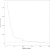 |
Fig. 4. Radial stellar density profile of cluster L38. The x-axis represents the distance to the cluster center and the y-axis the projected stellar number density. The vertical line marks the adopted cluster radius and the horizontal dashed line is the background density. |
For consistency with our previous work, we applied the cluster membership method used by our group in P09 and P15. The distance of each star from the center of the cluster, the RV, and the [Fe/H] are the parameters considered previously to establish whether the observed stars are likely members of the cluster or, conversely, whether they belong to the surrounding fields. Cluster members must be closer to the center than the adopted cluster radius. It is also expected that cluster stars have similar RV values within the RV dispersion expected for a cluster. Also, with a mean RV value being not necessarily similar to that of field stars and with a smaller dispersion. In addition, under the assumption that the clusters do not possess any intrinsic internal abundance dispersion, the observed dispersion in the cluster member metallicities should correspond to that expected from the individual metallicity errors. To illustrate our method, we show in Figs. 5 and 6 the behavior of the RV and metallicity of the red giant stars observed in the cluster L38 versus the distance from the cluster center, respectively.
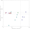 |
Fig. 5. Radial velocity vs. distance from the cluster center for L38 targets. Radial velocity cuts and the adopted cluster radius are marked with horizontal and vertical lines, respectively. The color code is the same as in Fig. 2. |
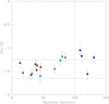 |
Fig. 6. Metallicity vs. distance from the cluster center for L38 targets. Metallicity cuts and the adopted cluster radius are marked with horizontal and vertical lines, respectively. The color code is the same as in Fig. 2. |
In Figs. 5 and 6, the vertical line marks the adopted cluster radius and the horizontal lines are the corresponding cuts in RV and metallicity adopted in this work. The RV cuts are the sum in quadrature of the expected dispersion within a cluster (∼5 km s−1, Pryor & Meylan 1993) and our error in the calculation of the RV values (∼7.5 km s−1) amounts to 9 km s−1. As we did in all our previous works, we rounded up our RV cuts to ±10 km s−1. The metallicity cuts (±0.20 dex) correspond to the mean error of our metallicity determination for the observed red giants. We also limited adopted cluster members to having v − vHB < +0.2 to avoid any possible effect on the metallicity due to the possible loss of linearity between v − vHB and ΣEW below the magnitude of the RC.
In order to improve our traditional membership analysis and to make sure we have selected stars with the maximum probability of being cluster members, we also analyzed the proper motions (PMs) of the observed stars. Using the corresponding cluster central coordinates, we searched for Gaia eDR3 (Gaia Collaboration 2021) stars in the area of each cluster. We then identified our targets in the Gaia eDR3 astrometric catalog and we discarded those stars whose motion is not consistent with the average motion of the cluster in the PM plane [μα, μδ] (Fig. 7). It is expected that cluster member stars have a similar movement within the uncertainties and the non-member stars present a greater dispersion in both coordinates. Therefore we discard those spectroscopic members with deviating PM with respect to the values that our spectroscopic members present.
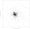 |
Fig. 7. Proper motion plane for cluster L38. Black points represent stars from the Gaia eDR3 catalogue and large circles stand for our spectroscopic targets. The color code is the same as in Fig. 2 |
The color code in the figures, which is explained in the caption of Fig. 2, is the same as in our previous work (Grocholski et al. 2006; P09; P15). Observed stars that have passed the cuts in radius, RV, metallicity, and PMs (red symbols) are considered our final cluster members. Figure 8 shows the CaT index ΣEW vs. v − vHB for stars observed in cluster L38, where the linear behavior of cluster member stars can be seen, in contrast to the field stars whose distribution has a larger scatter. In Fig. 9, we plot the complete sample, as in Fig. 8, but including only our final members in each cluster.
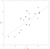 |
Fig. 8. Sum of the equivalent widths of the three CaT lines vs. v − vHB for identified members and non-members of cluster L38. The solid line represents the isometallicity line corresponding to the mean cluster metallicity. The color code is the same as in Fig. 2. |
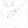 |
Fig. 9. Sum of the equivalent widths of the three CaT lines vs. v − vHB only for members stars in all our cluster sample. The dashed lines represent lines of equal metallicity of −0.6, −0.8, −1.0, −1.2, −1.4, and −1.6 dex from top to bottom. |
In Table 2 we list successively for the member stars of our cluster sample: the identification of the star, equatorial coordinates, heliocentric RV, v − vHB, ΣEW, and metallicity on the C04 scale, with their respective errors.
Measured values for member stars.
Using only cluster member stars, we then calculated the mean cluster RV and [Fe/H]. In Table 3, we present the cluster name in column (1) and the number n of stars that turned out to be cluster members in column (2), as well as the mean cluster RVs and metallicity, with their respective errors, in Cols. (3) and (4), respectively. We note that some clusters in our sample present smaller RV values (differences between ∼9 and ∼24 km s−1) than those obtained by Song et al. (2021). A possible source of discrepancy may include the correction due to the offset of the stars in the slits, whose values are of the order of the observed differences.
Derived cluster mean properties.
Although these differences do not affect our membership selection or the metallicity analysis presented here, they must be be considered when using our RVs for any dynamical analysis.
We summarize in Table 4 the most important previous metallicity determinations for our sample. In general terms, there is a reasonable agreement with the metallicity values previously determined by other authors.
Metallicity from the literature for our observed clusters.
5. Results and discussion
In order to analyze the chemical evolution of the SMC based on a statistical sample as large as possible and a set of homogeneously determined metallicities, we compiled all the clusters that have metallicities determined by the CaT technique from the literature. Besides the 12 clusters studied in the present work, we included in the sample the ones previously studied by Da Costa & Hatzidimitriou (1998, hereafter DH98), P09, P15, and D21. Thus we obtained a sample of 48 clusters with metallicities determined in a homogeneous way, which represents a 40% increase over the sample analyzed in P15. This sample also substantially improves our coverage of the different SMC components, naturally helping to clarify any individual trends. We present in Table 5 the adopted metallicity, age, semimajor axis, and component values for the additional cluster sample. With this extended cluster sample, we analyzed the MG, MD, and AMR in the SMC.
Extended cluster sample.
Two of the clusters in our sample (L11 and NGC 339) possess CaT metallicities from DH98. Both CaT determinations are in very good agreement in each case, showing that our metallicities are on the same scale as in their work. In addition, the sample analyzed here has one cluster in common with P15 (K44). For this cluster, we found a metallicity value of −0.78 ± 0.03, which is in very good agreement with the value derived by P15 (−0.81 ± 0.04) and based on completely independent data. This graphically confirms that our metallicities are also on the same scale as our previous works (including P09), which is to be expected considering that we used the same telescope, instrument, instrumental configuration, methods, and analysis. Our current sample has no clusters in common with D21. However, we do have a cluster in common (NGC 151) with Dias et al. (2022), which is based on observations taken with the same instrument and instrumental configuration as D21. Also, both works follow the same prescriptions and methods for the CaT metallicity determination. Therefore, the comparison with Dias et al. is an indirect comparison to D21. Dias et al. (2022) calculated a CaT metallicity of −0.75 ± 0.08, which is in excellent agreement with the value found in this work. Consequently, we consider that our full cluster sample is homogeneous with metallicities on the same scale.
Although our sample is homogeneous in terms of metallicity, it is necessary to note that it is heterogeneous in age, in the sense that the cluster data used in the literature to determine ages are variable in instrument and quality (from precise HST data to less precise ground-based data from small telescopes). Efforts to increase the cluster samples with homogeneous ages are being carried out by the VISCACHA survey (Maia et al. 2019, limiting magnitude V ∼ 24.5), which is aimed at deriving the ages of about half of the outer SMC clusters, among its multiple goals. The quality of the VISCACHA photometric data (obtained with the 4 m telescope SOAR and its adaptive optics module SAM) and the precision of the methods used to determine both ages and other astrophysical parameters have been demonstrated in a series of publications with important results for the SMC study (Maia et al. 2019; Santos et al. 2020, D21). Another important and complementary source of accurate photometry is the STEP survey (Ripepi et al. 2014, limiting magnitude g ∼ 24). This survey, performed with the VLT Survey Telescope (VST), covers the SMC Main Body, the bridge and part of the Magellanic Stream, allowing for the homogeneous determination of ages and structural parameters of a large cluster sample (Gatto et al. 2021).
We also emphasize that our cluster sample is not a magnitude- or mass-limited sample, nor is it complete in any sense. Therefore, a larger cluster sample will certainly reveal more details on the SMC chemical enrichment history.
5.1. Metallicity gradient
Overall, MGs are important tools for analyzing the chemical evolution of galaxies and their dynamical history (Ho et al. 2015). An examination of the MGs in nearby galaxies such as the MCs can help understand these processes in similar, more distant galaxies. Although there has been some discrepancy between spectroscopic and photometric studies regarding the existence of a MG in the SMC (Choudhury et al. 2020), the latest research tends to suggest that field stars clearly present such a gradient. The spectroscopic work on red giant branch stars based on CaT metallicities (Carrera et al. 2008, Dobbie et al. 2014b; P10; P16) agrees on the matter of the existence of a clear MG in the SMC field. Although field star photometric studies (Piatti 2012) and the photometry of variable stars (Kapakos et al. 2011; Haschke et al. 2012b) have not found any evidence of a field MG, the photometric metallicity maps created by Choudhury et al. (2018) and Choudhury et al. (2020) (using data from the Magellanic Cloud Photometric Survey (MCPS), the Optical Gravitational Lensing Experiment (OGLE III), and the near-infrared VISTA Survey (VMC)) have found evidence of metallicity trends in the SMC. In particular, Choudhury et al. (2020) confirm that the SMC field MG gradients are radially asymmetric.
While there seems to be a general agreement in the literature that SMC field stars present a MG, the situation is not as clear when cluster samples are analyzed. P15, using a sample of 29 SMC clusters, showed that it is not possible to find a statistically significant gradient in the inner region of the galaxy (a < 4°). This is in contrast to what is observed in the outer part of the galaxy (a > 4°), where the clusters present a behavior similar to that of field stars. In the external region of the SMC, both populations (clusters and fields) appear to present a positive MG with similar slopes. The difference in the behavior of clusters and field stars in the inner region of the SMC remains difficult to explain.
Figure 10 shows the behavior of metallicity as a function of the semimajor axis, a, for the complete sample. Pink and black symbols represent clusters included in Tables 3 and 5, respectively. In this figure, the breakpoint found by D21 using the cluster radial density profile is marked with the solid vertical line ( ). Massana et al. (2020) calculated that the tidal radius for the SMC is ∼4.5° based on the SMC and LMC masses and their relative distance. We adopted the value from D21 as the distance from the SMC center to divide it into what we call the internal and external regions because this distance is based on star clusters and is consistent with an independent calculation of the SMC tidal radius. In Fig. 10, it can be clearly seen that with this extended sample, and using the projected distances adopted in this work, the metallicity spread is even larger in the internal region of the SMC with respect to P15.
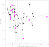 |
Fig. 10. Metallicity as a function of the semimajor axis, a, for the full cluster sample. Black circles are clusters taken from the literature (Table 5) and pink squares are clusters studied in this work (Table 3). Vertical solid and dashed lines represent the SMC tidal radius and the errors from D21. The MG fits are shown for the inner and outer regions (solid lines). |
We fit straight lines to the inner and outer regions, dividing at 3.4° (solid lines in Fig. 10), and we found values for the MG of −0.08 ± 0.04 dex deg−1 and 0.03 ± 0.02 dex deg−1, respectively. Clusters were equally weighted in making the fits. These values and their corresponding errors are consistent with the absence of a MG in the outer region. Although the MG value obtained in the inner region is in agreement with that obtained for the field stars, −0.075 ± 0.011 dex deg−1 (Dobbie et al. 2014b) and −0.08 ± 0.02 dex deg−1 (P16), it has an error of 50% due to the large range in metallicities (> 0.6 dex) that the clusters cover in that region.
P15 drew attention to a possible inversion of the metallicity gradient (an aspect that they named the V-shape) in the external region of the SMC (beyond 4°), which can also be seen in the compiled sample of clusters from the catalog of Bica et al. (2020). The V-shape is even more evident in SMC field stars studied with CaT (P16) but the field photometric study of Choudhury et al. (2020) found that the metallicity rises to an almost constant value of −0.93 dex from ∼3.5° to 4° (it is necessary to take into account that the definition of a used by Choudhury et al. 2020 is not exactly the same as in this work). Significantly, the farthest cluster in our sample (L116) belongs to the Southern Bridge and has a metallicity of −0.89, which is similar to the approximately constant metallicity in the outer regions found by Choudhury et al. (2020). If we consider the full cluster sample as in Fig. 10, the MG in the outer region appears to become flat, with a high dispersion, and the V-shape appears to be slightly diluted.
In Fig. 11, we plot the same data as in Fig. 10, but we use symbols with different colors according to the definition adopted in this work (see the caption of Fig. 11). One of the most conspicuous aspects of this figure is the fact that the only group of clusters that presents a particularly well-defined gradient or traces the V-shape in a clear way are those belonging to the Northern Bridge. It is interesting to note, however, that all components show a minimum in metallicity as well as metallicity dispersion near the tidal radius (∼0.2 dex) and that the dispersion grows considerably as we move away from this radius (∼0.6 dex), both in the internal and external regions. Although the number of clusters in the Northern Bridge region that are present in our sample is still small, we do get the impression that it is the only group that shows a V-shape, with a vertex approximately coincident with the tidal radius and an inversion of the gradient in the external region. D16 and Bica et al. (2020) argue that the V-shape is intrinsic to the Wing/Bridge region. In fact, the analysis that D16 carried out on a sample of clusters belonging to the West Halo does not show such an inversion, although the number of clusters in their West Halo sample beyond 4° is very small.
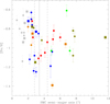 |
Fig. 11. Metallicity as a function of the semimajor axis, a, for the full cluster sample but symbols colored according to the adopted classification (D14, D16 and D21): grey, orange, blue, green, red, and brown symbols represent clusters belonging to the Main Body, Counter-Bridge, West Halo, Wing/Bridge, Northern Bridge, and Southern Bridge, respectively. Squares depict the clusters studied in this paper and circles represent our additional cluster sample. |
Clusters belonging to the Northern Bridge classification have been graphed separately in Fig. 12, showing a different radial range than in Figs. 10 and 11 for a better visualization. The fits corresponding to the regions internal and external to the tidal radius are shown with solid lines in the figure. We found values of −0.42 ± 0.15 dex deg−1 and 0.09 ± 0.03 dex deg−1 for the inner and outer region, respectively. The fit corresponding to the internal region in the Northern Bridge is not well constrained due to the low number of clusters. However, the external region presents a clear and much more robust indication of a positive gradient, which would be interesting to further investigate with a larger sample. Mergers, interactions, and radial migration could flatten or invert the metallicity radial gradient (e.g., Tissera et al. 2016).
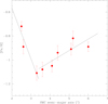 |
Fig. 12. Metallicity as a function of the semimajor axis, a, only for Northern Bridge clusters. Solid lines show the data fits inside and outside the tidal radius. We note that the radial range is smaller than that shown in Figs. 10 and 11. |
As mentioned previously, D16 analyzed the chemical properties of the West Halo. They made a photometric determination of the ages and metallicities of 9 clusters belonging to the West Halo, and supplemented their sample with 13 other clusters in the same region studied by other authors. Using that extended sample, they argued in favor of the existence not only of an MG, but also of an AG. The sample that these authors analyze includes metallicities determined with a variety of techniques and substantial differences in the quality of the data used in the compiled works, and thus their results are unfortunately plagued by inhomogeneity. For this reason, the MG results from D16 are based on a sample of clusters with metallicities determined in an inhomogeneous way. Our sample includes 12 West Halo clusters, two that are in common with D16: NGC 152 and K8. D16 found metallicity value of −0.87 ± 0.07 for NGC 152, close to the value derived in this work (−0.72 ± 0.04); however, in the case of K8, D16 found a substantially more metal-poor value (−1.12 ± 0.15) than in P15 (−0.70 ± 0.04).
In order to analyze the existence of gradients in the West Halo with a sample of clusters observed and studied in the same way and with precise metallicities on the same scale, we plot the sample that belongs to that region in Figs. 13 and 14. We compare our homogeneous data with the fits derived by D16, which can be seen in the figures indicated by solid lines. They performed fits to three different samples: clusters collected from the literature (blue line, −0.13 ± 0.08 dex deg−1, 2.5 ± 0.8 Gyr deg−1), clusters analyzed in their paper (red line, −0.34 ± 0.21 dex deg−1, 1.9 ± 0.6 Gyr deg−1), and all the clusters together (black line −0.19 ± 0.09 dex deg−1, 2.6 ± 0.6 Gyr deg−1). The linear fit to our complete West Halo sample yields a value of −0.09 ± 0.07 dex deg−1 (dashed line). This value is in agreement with the MG for field stars but with an error of 78%. If we consider only clusters within the 3.4 degrees from the SMC center, we obtain a MG of −0.19 ± 0.43 dex deg−1 (dotted line). Although the value of the slope in the inner region is compatible with that found by D16 for their entire sample, our determination has a very large error. The uncertainties of the MG in our West Halo sample are of course affected by the considerable metallicity dispersion in the inner region.
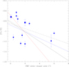 |
Fig. 13. Metallicity as a function of the semimajor axis, a, only for the West Halo clusters in our sample. Squares are clusters studied in the present work and circles are those taken from the literarure. Solid lines are the fits from D16 and dashed and dotted lines are the fits to our data. We note that the radial range is smaller than that shown in Figs. 10 and 11. |
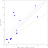 |
Fig. 14. Age as a function of the semimajor axis, a, for the West Halo clusters in our sample. The symbols are the same as in Fig. 13. The solid lines are the fits from D16 and the dashed line shows the fit to our data. |
Regarding the AG, we observe in Fig. 14 that our West Halo sample shows a clear tendency for the clusters to be older as the distance to the galaxy center increases. The fit to our data gives a value for the AG of 2.7 ± 0.8 Gyr deg−1, in very good agreement with that found by D16 for their full sample.
While the latest photometric work investigating the age and metallicity gradients in the SMC through its star cluster system (e.g., Narloch et al. 2021) suggests that the more metal-rich clusters are concentrated in the inner regions of the galaxy, our spectroscopic data show that the situation is more complicated. Although there seems to be a tendency for the clusters to be more metal-poor as we move away from the center of the SMC and out to 3.4°, the dispersion of metallicities in the inner region is quite large, decreasing the significance of the linear fit.
D16 defined the Main Body as the region with a < 2° based on visual criteria. However, taking into account both the results found here and those from Dias et al. (2021), we consider that this region should be defined by a more astrophysical criterion such as the tidal radius. According to our results, we consider that it is reasonable to redefine the Main Body region as the one contained within a ellipse with a semimajor axis of 3.4°, using D21’s tidal radius value as our criterion.
5.2. Metallicity distribution
The MD of a galaxy’s stellar populations contains relevant information to understand different astrophysical processes related to its evolutionary history, such as the star formation history, gas flows, and chemical enrichment (e.g., Kirby et al. 2013; Leaman et al. 2013; Fukagawa 2020, for dwarf galaxies). A possible bimodality in the SMC’s cluster MD was suggested by P15. Based on a sample of 35 clusters with homogeneously determined CaT metallicities, they found a probability of 86% that the cluster MD is bimodal, with possible peaks at −1.1 and −0.8 dex. This is contrary to what has been suggested in other studies (e.g., Bica et al. 2020). This latter study, based on a compilation of a large number of SMC and Magellanic Bridge clusters, found that the MD is unimodal, with a peak between −0.8 and −1.0. On the other hand, several studies have shown that the field metallicity distribution is unimodal with a peak between ∼ − 0.94 to ∼ − 1 dex (e.g., Carrera et al. 2008, P10, Dobbie et al. 2014b, P16, Choudhury et al. 2018, 2020).
Using the sample analyzed in this work, we applied the Gaussian Mixture Model (GMM, Muratov & Gnedin 2010) in order to analyse the possible bimodality in the MD. The unimodal fit gives μ = −0.913 and σ = 0.178. The bimodal fit (heteroscedastic split) gives μ1 = −0.806, μ2 = −1.072, σ1 = 0.105 yr, and σ2 = 0.140, with a p value of 0.476. This means that there is a 47.6% probability of being wrong in rejecting unimodality. The parametric bootstrap gives a probability of 58.7% that the MD is bimodal. The calculated separation of the peaks and the kurtosis value are 2.86 ± 0.89 and 0.476, respectively, compatible with a unimodal distribution. This means that with a larger cluster sample a bimodal MD is less significant than that found in P15. Our cluster MD, together with the unimodal (red line) and bimodal (blue line) fits are shown in Fig. 15. We note that the GMM algorithm does not use the bin size of the histogram to make the probability calculations.
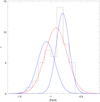 |
Fig. 15. Metallicity distribution of our enlarged SMC cluster sample (Tables 3 and 5). The fits derived from the application of the GMM algorithm are shown in red (unimodal fit) and blue (bimodal fit). The GMM method is independent of the bin size used for plotting the histogram. |
5.3. Age-metallicity relation
The AMR is a potentially very useful tool to analyze the chemical history of a galaxy, providing hints on possible chemical enrichment processes. Various efforts have been made in recent decades to try to establish the AMR of the SMC, using as tracers both star clusters and field stars. Various models of chemical evolution have been proposed in the literature to explain the history of chemical evolution of the SMC. We found in our previous investigations, using a sample of 29 clusters (P09; P15), that there is no unique AMR in the SMC and that at a given age there is a dispersion of metallicities of 0.5 dex. This value cannot be explained by the errors involved in the calculation of metallicities, which are significantly lower. This dispersion of metallicities can also be observed in photometric studies of the SMC AMR (for example, Perren et al. 2017; Narloch et al. 2021).
We compare now in Fig. 16 our enlarged cluster sample with the different models. The theoretical bursting model (Pagel & Tautvaisiene 1998, PT98) burst followed by a long period with no chemical enrichment (between 11 and 4 Gyr ago) and a more recent star formation burst that could have increased the metallicity in the SMC to its present value. It is necessary to emphasize that the PT98 model predicts basically no star formation between the ages of ∼12 Gyr and ∼3 − 4 Gyr, which conflicts with the existence of clusters and field stars in that age range. An AMR model not only needs to fit the observational AMR, but it also needs to be consistent with the observed star formation history (SFH). The closed box model proposed by DH98, from the CaT analysis of six clusters distributed throughout the spatial extent of the SMC, suggests a continuous and gradual chemical enrichment throughout the life of the SMC. The AMR from Harris & Zaritsky (2004, HZ04) is derived from the SFH analysis in 351 regions in the SMC across the central area of the Main Body (4° × 4.5°). The AMR proposed by Carrera et al. (2008, C08) comes from the CaT study of 350 red giant stars in 13 fields located between ∼1° and 4° from the SMC center. Cignoni et al. (2013) proposed two AMR models (C13-C, C13-B) from the SFH of 4 fields, observed with the HST, located in the Main Body and the wing of the SMC, 0.5–2° from the galaxy center. The three models from Tsujimoto & Bekki (2009) represent merger models with a mass radio of 1:1 (TB09-1:1) and 1:4 (TB09-1:4), and with no merger (TB08-nm). Perren et al. (2017, hereafter Pe17) homogeneously analyzed a sample of 89 SMC clusters that are spatially distributed throughout a large area of the galaxy, using data in the Washington photometric system and the Automated Stellar Cluster Analysis (ASteCA) package (Perren et al. 2015). They proposed a model of chemical evolution with the metallicity decreasing towards older ages up to approximately 3 Gyr ago, similar to what is predicted by other models but moving towards higher metallicities. Their model resembles the AMRs proposed for field stars by HZ04 and Cignoni et al. (2013, C13-C and C13-B) but shifted in metallicity to higher values.
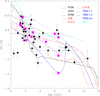 |
Fig. 16. Metallicity as a function of age for the complete cluster sample. Magenta squares are the clusters analyzed in this paper. Black circles represent the additional sample of clusters with homogeneously derived spectroscopic metallicities. The observational data are compared with different models of chemical evolution available in the literature. The reference for each model is given in the inset. |
In Fig. 16, we can see that our conclusions do not change substantially with this larger sample with respect to those reached in our previous work. For ages less than 4 Gyr, clusters appear to have undergone chemical enrichment similar to that predicted by the bursting model, with the exception of two clusters (K9 and IC1708). These two objects have a considerably lower metallicity than predicted by any model for their ages. The cluster sample older than 4 Gyr presents a considerable dispersion of metallicities that show no agreement with any of the proposed chemical evolution models. We note that the addition of our most metal-poor cluster firms up the establishment of a metallicity spread at around 6.5 Gyr, now almost approaching 0.6 dex, and thus presenting an intriguing aspect of our study.
As in the previous section, we analyzed the AMR by separating the cluster sample according to the classification proposed by D16 and D21, which can be seen in Fig. 17. The first observation that stands out from this figure is that the Main Body, Counter-Bridge, and Northern Bridge would not seem to present a clear AMR, each covering a wide range of ages and metallicities. Additionally, the West Halo clusters for which D16 photometrically found an AMR compatible with the bursting model appear to follow the closed box model (DH98), according to our data, with the exception of two points. The clusters belonging to the Wing/Bridge and Southern Bridge, whose AMR has been graphed separately in Fig. 18, seem to share the same chemical evolution, although it is difficult to make a conclusive assessment due to the low number of Wing/Bridge and Southern Bridge clusters present in our sample. Assuming that the SMC does have a unique AMR in both those regions, it would seem to follow the predictions of the bursting model but with metallicity values higher than those expected for clusters older than 3–4 Gyr. In fact, in these regions, the model of chemical evolution in that SMC region appears to be an intermediate model between those of Pagel & Tautvaisiene (1998, PT98) and Pe17. These two models predict a similar chemical enrichment history, but displaced relative to each other in metallicity, mainly at intermediate ages before the possible burst of star formation 4 Gyr ago. A precisely intermediate model between these two scenarios, which would seem to fit approximately the data, is that of Tsujimoto & Bekki (2009) corresponding to a 1:1 merger. Alternatively, the two AMRs proposed by Cignoni et al. (2013) reproduce the data well. Particularly interesting are the C13-B and C13-C models, which were fitted to the Main Body and wing using HST data.
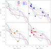 |
Fig. 17. Metallicity as a function of age for the complete cluster sample but divided according to the classifications of D16 and D21. The color code is explained in Fig. 11 and in the text. |
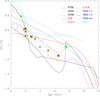 |
Fig. 18. Metallicity as a function of age for Wing/Bridge and Southern Bridge clusters. |
We trust that with a database of clusters with homogeneous metallicities and ages, and with the accuracy provided by the CaT technique as well as the VISCACHA and STEP data, it will be possible to disentangle the AMR in a more precise way, especially in the intermediate age range, if indeed it can be disentangled. Also, the observation of a larger number of clusters in the Wing/Bridge and Southern Bridge regions would be necessary to corroborate the possible AMR they have in common. On the other hand, the SMC may simply prove to be complicated and challenge simple assumptions. With the exception of the TB09 models, the proposed AMRs assume that the SMC did not experience accretion and mergers, whereas its highly disturbed shape may also be the result of a merger (Bekki & Chiba 2008; Tsujimoto & Bekki 2009; Pieres et al. 2017). If so, more metal-poor clusters at a given age might be derived from a smaller, more metal-poor dIrr that merged with the early SMC, partly producing the cluster metallicity dispersion that we observe. Furthermore, recent works, such as that described in, for example, Li et al. (2021) and Li et al. (in prep), suggest that even in a dwarf galaxy like the SMC, the correlation length scale for abundance enrichment is still substantially smaller than the galaxy’s size. Consequently, supernova enrichment products are not expected to have been homogeneously mixed through the entire SMC. Moreover, Nidever et al. (2020) found that the SMC has had a very low star formation efficiency, even in comparison with other less massive dwarf galaxies when comparing the [α/Fe] versus [Fe/H] trends assuming that the efficiency should increase with galaxy mass. Therefore, the substantial spread in cluster abundances at fixed age is not unexpected. This does not rule out, however, the possibility of infall (and incomplete mixing) of pristine (or at least low abundance) gas, potentially connected to the SMC/LMC interaction history and contributing to the range in cluster abundances at fixed age.
Finally, it is necessary to bear in mind that the definition of D16 is an initial classification based on the projected position of the clusters without considering any information on the dynamics of the clusters. We need to know the cluster orbits in order to analyze possible superposition of different timescales in the same region. So far, no SMC cluster orbits have been calculated, but they will be part of a future work. The full kinematics of the SMC clusters has only recently started to be mapped (e.g., D21, Piatti 2021; Dias et al. 2022).
6. Summary and conclusions
We present radial velocites (RVs) and calcium triplet metallicities (CaT) for a large sample of red giant stars in 12 SMC clusters. We derived mean cluster RVs and metallicities, with a mean error of 2.1 km s−1 and 0.03 dex, respectively. Using this information, together with that available in the literature for another 36 clusters with CaT metallicities derived homogeneously, we analyzed the metallicity gradient, the metallicity distribution, and the age-metallicity relation in the SMC. Clusters of the final sample are distributed over an area of ∼70 deg2 with 0.4 Gyr ≤ Age ≤ 10.5 Gyr. This is the largest sample of spectroscopically analyzed SMC clusters available to date. Following the ideas of Dias et al. (2016a) and Dias et al. (2021), we divided the sample in six groups: Main Body, Counter-Bridge, Wing/Bridge, Northern Bridge, Southern Bridge, and West Halo. In addition, we adopted the value of the SMC breakpoint derived by Dias et al. (2021) ( ) to divide the galaxy into what we call the inner and outer regions. We can summarize our results as follows:
-
We confirm that in the inner region (inside 3.4°) the SMC clusters present a considerable dispersion of metallicity (∼ 0.6 dex).
-
Clusters in the inner region exhibit a metallicity gradient with a value compatible with that shown by field stars but with an error of 50% due to the large dispersion of metallicities. On the other hand, our data show that the outer region does not present a significant MG.
-
Concerning the components suggested by Dias et al., we observed that only the clusters belonging to the Northern Bridge appear to trace a V-Shape metallicity gradient, showing a clear inversion near the tidal radius of the SMC. However, all the groups present a minimum in the metallicities at a distance from the center of the galaxy that coincides with the tidal radius proposed by Dias et al. (2021).
-
Our sample of West Halo clusters shows a clear age gradient, in agreement with Dias et al. (2016a). Regarding the MG we found a value compatible with the one derived for field stars (e.g., Parisi et al. 2016; Dobbie et al. 2014b) and with the MG derived by Dias et al. (2016a) for the West Halo, depending on whether we are considering all of our West Halo clusters or only those located in the inner region.
-
The differences in the behavior of the metallicity gradient inside and outside the tidal radius, as well as the differences found analyzing the different groups defined by Dias et al. (2016a) and Dias et al. (2021), suggest that the chemical history of the SMC strongly depends on its dynamical history, as was previously emphasized by those authors. Also, according to these results, we propose that the Main Body region be extended out to 3.4°.
-
The application of the Gaussian mixture model (Muratov & Gnedin 2010) to the metallicity distribution of our entire cluster sample points to the probability that our cluster metallicity distribution is much less bimodal than was previously found by Parisi et al. (2015).
-
With respect to the age-metallicity relation, clusters younger than 4 Gyr appear to follow the bursting model of Pagel & Tautvaisiene (1998). For intermediate ages, no model adequately reproduces the data and the dispersion of metallicities becomes even more evident. The development of theoretical models that reproduce the observations and also satisfy the SMC cluster and field star SFHs are essential for a complete understanding of the chemical evolution of this galaxy. We hope that our results will be an inspiration in that sense.
-
Clusters belonging to the Wing/Bridge and Southern Bridge exhibit a well-defined age-metallicity relation with relatively little scatter in abundance at fixed age compared to the other regions. Although the sample is small, both groups appear to share a common chemical enrichment history. Our data also suggest that the West Halo clusters could follow the closed box model proposed by Da Costa & Hatzidimitriou (1998).
-
The lack of a clear age-metallicity relation for the SMC as a whole, and the large spread of metallicities at any given age, could indicate that mergers, including gas infall, played a role during its history, in addition to the interaction with the LMC.
Acknowledgments
This work is based on observations collected at the European Southern Observatory, Chile, under Program 075.B-0548 and 073.B-0488. This work presents results from the European Space Agency (ESA) space mission Gaia. Gaia data are being processed by the Gaia Data Processing and Analysis Consortium (DPAC). Funding for the DPAC is provided by national institutions, in particular the institutions participating in the Gaia MultiLateral Agreement (MLA). The Gaia mission website is https://www.cosmos.esa.int/gaia. The Gaia archive website is https://archives.esac.esa.int/gaia. We thank the referee for comments that helped to improve this work. This research was partially supported by the Argentinian institution SECYT (Universidad Nacional de Córdoba). D.G. gratefully acknowledges support from the Chilean Centro de Excelencia en Astrofísica y Tecnologías Afines (CATA) BASAL grant AFB-170002. D.G. also acknowledges financial support from the Dirección de Investigación y Desarrollo de la Universidad de La Serena through the Programa de Incentivo a la Investigación de Académicos (PIA-DIDULS).
References
- Armandroff, T. E., & Da Costa, G. S. 1991, AJ, 101, 1329 [Google Scholar]
- Armandroff, T. E., & Zinn, R. 1988, AJ, 96, 92 [Google Scholar]
- Bekki, K., & Chiba, M. 2008, ApJ, 679, L89 [NASA ADS] [CrossRef] [Google Scholar]
- Belokurov, V., Erkal, D., Deason, A. J., et al. 2017, MNRAS, 466, 4711 [Google Scholar]
- Belokurov, V. A., & Erkal, D. 2019, MNRAS, 482, L9 [Google Scholar]
- Besla, G. 2011, PhD Thesis, Harvard University [Google Scholar]
- Besla, G., Kallivayalil, N., Hernquist, L., et al. 2007, ApJ, 668, 949 [Google Scholar]
- Besla, G., Kallivayalil, N., Hernquist, L., et al. 2010, ApJ, 721, L97 [Google Scholar]
- Besla, G., Kallivayalil, N., Hernquist, L., et al. 2012, MNRAS, 421, 2109 [Google Scholar]
- Besla, G., Martínez-Delgado, D., van der Marel, R. P., et al. 2016, ApJ, 825, 20 [Google Scholar]
- Bica, E., Dottori, H., & Pastoriza, M. 1986, A&A, 156, 261 [NASA ADS] [Google Scholar]
- Bica, E., Bonatto, C., Dutra, C. M., & Santos, J. F. C. 2008, MNRAS, 389, 678 [Google Scholar]
- Bica, E., Westera, P., Kerber, L. D. O., et al. 2020, AJ, 159, 82 [Google Scholar]
- Bitsakis, T., González-Lópezlira, R. A., Bonfini, P., et al. 2018, ApJ, 853, 104 [Google Scholar]
- Carretta, E., & Gratton, R. G. 1997, A&AS, 121, 95 [NASA ADS] [CrossRef] [EDP Sciences] [Google Scholar]
- Carrera, R., Gallart, C., Pancino, E., & Zinn, R. 2007, AJ, 134, 1298 [NASA ADS] [CrossRef] [Google Scholar]
- Carrera, R., Gallart, C., Aparicio, A., et al. 2008, AJ, 136, 1039 [Google Scholar]
- Carrera, R., Pancino, E., Gallart, C., & del Pino, A. 2013, MNRAS, 434, 1681 [NASA ADS] [CrossRef] [Google Scholar]
- Choudhury, S., Subramaniam, A., Cole, A. A., & Sohn, Y. J. 2018, MNRAS, 475, 4279 [NASA ADS] [CrossRef] [Google Scholar]
- Choudhury, S., de Grijs, R., Rubele, S., et al. 2020, MNRAS, 497, 3746 [NASA ADS] [CrossRef] [Google Scholar]
- Cignoni, M., Cole, A. A., Tosi, M., et al. 2013, ApJ, 775, 83 [Google Scholar]
- Cioni, M. R. L. 2009, A&A, 506, 1137 [NASA ADS] [CrossRef] [EDP Sciences] [Google Scholar]
- Cole, A. A., Smecker-Hane, T. A., Tolstoy, E., Bosler, T. L., & Gallagher, J. S. 2004, MNRAS, 347, 367 [NASA ADS] [CrossRef] [Google Scholar]
- Da Costa, G. S. 1991, in The Magellanic Clouds, eds. R. Haynes, & D. Milne, 148, 183 [CrossRef] [Google Scholar]
- Da Costa, G. S. 2016, MNRAS, 455, 199 (DC16) [CrossRef] [Google Scholar]
- Da Costa, G. S., & Hatzidimitriou, D. 1998, AJ, 115, 1934 [Google Scholar]
- de Freitas Pacheco, J. A., Barbuy, B., & Idiart, T. 1998, A&A, 332, 19 [NASA ADS] [Google Scholar]
- De Leo, M., Carrera, R., Noël, N. E. D., et al. 2020, MNRAS, 495, 98 [Google Scholar]
- Dias, B., & Parisi, M. C. 2020, A&A, 642, A197 [EDP Sciences] [Google Scholar]
- Dias, B., Coelho, P., Barbuy, B., Kerber, L., & Idiart, T. 2010, A&A, 520, A85 [NASA ADS] [CrossRef] [EDP Sciences] [Google Scholar]
- Dias, B., Kerber, L. O., Barbuy, B., et al. 2014, A&A, 561, A106 [NASA ADS] [CrossRef] [EDP Sciences] [Google Scholar]
- Dias, B., Kerber, L., Barbuy, B., Bica, E., & Ortolani, S. 2016a, A&A, 591, A11 [NASA ADS] [CrossRef] [EDP Sciences] [Google Scholar]
- Dias, B., Barbuy, B., Saviane, I., et al. 2016b, A&A, 590, A9 [NASA ADS] [CrossRef] [EDP Sciences] [Google Scholar]
- Dias, B., Angelo, M. S., Oliveira, R. A. P., et al. 2021, A&A, 647, L9 [NASA ADS] [CrossRef] [EDP Sciences] [Google Scholar]
- Dias, B., Parisi, M. C., Angelo, M., et al. 2022, MNRAS, 512, 4334 [NASA ADS] [CrossRef] [Google Scholar]
- Diaz, J., & Bekki, K. 2011, MNRAS, 413, 2015 [Google Scholar]
- Diaz, J. D., & Bekki, K. 2012, ApJ, 750, 36 [Google Scholar]
- Dobbie, P. D., Cole, A. A., Subramaniam, A., & Keller, S. 2014a, MNRAS, 442, 1663 [Google Scholar]
- Dobbie, P. D., Cole, A. A., Subramaniam, A., & Keller, S. 2014b, MNRAS, 442, 1680 [NASA ADS] [CrossRef] [Google Scholar]
- D’Onghia, E., & Fox, A. J. 2016, ARA&A, 54, 363 [CrossRef] [Google Scholar]
- Dopita, M. A., Vassiliadis, E., Wood, P. R., et al. 1997, ApJ, 474, 188 [NASA ADS] [CrossRef] [Google Scholar]
- Durand, D., Hardy, E., & Melnick, J. 1984, ApJ, 283, 552 [NASA ADS] [CrossRef] [Google Scholar]
- El Youssoufi, D., Cioni, M.-R. L., Bell, C. P. M., et al. 2021, MNRAS, 505, 2020 [NASA ADS] [CrossRef] [Google Scholar]
- Evans, C. J., & Howarth, I. D. 2008, MNRAS, 386, 826 [CrossRef] [Google Scholar]
- Friel, E. D., Janes, K. A., Tavarez, M., et al. 2002, AJ, 124, 2693 [NASA ADS] [CrossRef] [Google Scholar]
- Fukagawa, N. 2020, MNRAS, 491, 1759 [NASA ADS] [CrossRef] [Google Scholar]
- Gaia Collaboration (Prusti, T., et al.) 2016, A&A, 595, A1 [NASA ADS] [CrossRef] [EDP Sciences] [Google Scholar]
- Gaia Collaboration (Luri, X., et al.) 2021, A&A, 649, A7 [EDP Sciences] [Google Scholar]
- Gatto, M., Ripepi, V., Bellazzini, M., et al. 2021, MNRAS, 507, 3312 [NASA ADS] [CrossRef] [Google Scholar]
- Glatt, K., Gallagher, J. S. I., Grebel, E. K., et al. 2008a, AJ, 135, 1106 [NASA ADS] [CrossRef] [Google Scholar]
- Glatt, K., Grebel, E. K., Sabbi, E., et al. 2008b, AJ, 136, 1703 [Google Scholar]
- Glatt, K., Grebel, E. K., & Koch, A. 2010, A&A, 517, A50 [CrossRef] [EDP Sciences] [Google Scholar]
- Glatt, K., Grebel, E. K., Jordi, K., et al. 2011, AJ, 142, 36 [NASA ADS] [CrossRef] [Google Scholar]
- Graczyk, D., Pietrzyński, G., Thompson, I. B., et al. 2020, ApJ, 904, 13 [Google Scholar]
- Grocholski, A. J., Cole, A. A., Sarajedini, A., Geisler, D., & Smith, V. V. 2006, AJ, 132, 1630 [NASA ADS] [CrossRef] [Google Scholar]
- Harris, J., & Zaritsky, D. 2004, AJ, 127, 1531 [NASA ADS] [CrossRef] [Google Scholar]
- Haschke, R., Grebel, E. K., & Duffau, S. 2012a, AJ, 144, 107 [NASA ADS] [CrossRef] [Google Scholar]
- Haschke, R., Grebel, E. K., Duffau, S., & Jin, S. 2012b, AJ, 143, 48 [NASA ADS] [CrossRef] [Google Scholar]
- Ho, I. T., Kudritzki, R.-P., Kewley, L. J., et al. 2015, MNRAS, 448, 2030 [NASA ADS] [CrossRef] [Google Scholar]
- Husser, T.-O., Latour, M., Brinchmann, J., et al. 2020, A&A, 635, A114 [NASA ADS] [CrossRef] [EDP Sciences] [Google Scholar]
- Irwin, M. J., Kunkel, W. E., & Demers, S. 1985, Nature, 318, 160 [Google Scholar]
- Jacyszyn-Dobrzeniecka, A. M., Soszyński, I., Udalski, A., et al. 2020, ApJ, 889, 25 [Google Scholar]
- Kallivayalil, N., van der Marel, R. P., & Alcock, C. 2006a, ApJ, 652, 1213 [NASA ADS] [CrossRef] [Google Scholar]
- Kallivayalil, N., van der Marel, R. P., Alcock, C., et al. 2006b, ApJ, 638, 772 [NASA ADS] [CrossRef] [Google Scholar]
- Kallivayalil, N., van der Marel, R. P., Besla, G., Anderson, J., & Alcock, C. 2013, ApJ, 764, 161 [Google Scholar]
- Kapakos, E., Hatzidimitriou, D., & Soszyński, I. 2011, MNRAS, 415, 1366 [NASA ADS] [CrossRef] [Google Scholar]
- Kayser, A., Grebel, E. K., Harbeck, D. R., et al. 2007, in Stellar Populations as Building Blocks of Galaxies. eds. A. Vazdekis, & R. Peletier, 241, 351 [NASA ADS] [Google Scholar]
- Kirby, E. N., Cohen, J. G., Guhathakurta, P., et al. 2013, ApJ, 779, 102 [Google Scholar]
- Lagioia, E. P., Milone, A. P., Marino, A. F., & Dotter, A. 2019, ApJ, 871, 140 [NASA ADS] [CrossRef] [Google Scholar]
- Leaman, R., Venn, K. A., Brooks, A. M., et al. 2013, ApJ, 767, 131 [NASA ADS] [CrossRef] [Google Scholar]
- Li, C., de Grijs, R., Deng, L., et al. 2016, Nature, 529, 502 [NASA ADS] [CrossRef] [Google Scholar]
- Li, Z., Krumholz, M. R., Wisnioski, E., et al. 2021, MNRAS, 504, 5496 [NASA ADS] [CrossRef] [Google Scholar]
- Livanou, E., Dapergolas, A., Kontizas, M., et al. 2013, A&A, 554, A16 [NASA ADS] [CrossRef] [EDP Sciences] [Google Scholar]
- Mackey, D., Koposov, S., Da Costa, G., et al. 2018, ApJ, 858, L21 [Google Scholar]
- Maia, F. F. S., Dias, B., Santos, J. F. C., et al. 2019, MNRAS, 484, 5702 [Google Scholar]
- Martocchia, S., Bastian, N., Usher, C., et al. 2017, MNRAS, 468, 3150 [NASA ADS] [CrossRef] [Google Scholar]
- Martocchia, S., Kamann, S., Saracino, S., et al. 2020, MNRAS, 499, 1200 [NASA ADS] [CrossRef] [Google Scholar]
- Massana, P., Noël, N. E. D., Nidever, D. L., et al. 2020, MNRAS, 498, 1034 [Google Scholar]
- Mathewson, D. S., Cleary, M. N., & Murray, J. D. 1974, ApJ, 190, 291 [NASA ADS] [CrossRef] [Google Scholar]
- Mauro, F., Moni Bidin, C., Geisler, D., et al. 2014, A&A, 563, A76 [NASA ADS] [CrossRef] [EDP Sciences] [Google Scholar]
- Mighell, K. J., Sarajedini, A., & French, R. S. 1998, AJ, 116, 2395 [Google Scholar]
- Mould, J. R., Jensen, J. B., & Da Costa, G. S. 1992, ApJS, 82, 489 [NASA ADS] [CrossRef] [Google Scholar]
- Muller, E., & Bekki, K. 2007, MNRAS, 381, L11 [NASA ADS] [CrossRef] [Google Scholar]
- Muratov, A. L., & Gnedin, O. Y. 2010, ApJ, 718, 1266 [Google Scholar]
- Muraveva, T., Subramanian, S., Clementini, G., et al. 2018, MNRAS, 473, 3131 [Google Scholar]
- Narloch, W., Pietrzyński, G., Gieren, W., et al. 2021, A&A, 647, A135 [NASA ADS] [CrossRef] [EDP Sciences] [Google Scholar]
- Nayak, P. K., Subramaniam, A., Choudhury, S., Indu, G., & Sagar, R. 2016, MNRAS, 463, 1446 [NASA ADS] [CrossRef] [Google Scholar]
- Nayak, P. K., Subramaniam, A., Choudhury, S., & Sagar, R. 2018, A&A, 616, A187 [NASA ADS] [CrossRef] [EDP Sciences] [Google Scholar]
- Nidever, D. L., Majewski, S. R., & Butler Burton, W. 2008, ApJ, 679, 432 [Google Scholar]
- Nidever, D. L., Majewski, S. R., Butler Burton, W., & Nigra, L. 2010, ApJ, 723, 1618 [NASA ADS] [CrossRef] [Google Scholar]
- Nidever, D. L., Olsen, K., Walker, A. R., et al. 2017, AJ, 154, 199 [Google Scholar]
- Nidever, D. L., Price-Whelan, A. M., Choi, Y., et al. 2019, ApJ, 887, 115 [NASA ADS] [CrossRef] [Google Scholar]
- Nidever, D. L., Hasselquist, S., Hayes, C. R., et al. 2020, ApJ, 895, 88 [Google Scholar]
- Niederhofer, F., Cioni, M. R. L., Rubele, S., et al. 2018, A&A, 613, L8 [NASA ADS] [CrossRef] [EDP Sciences] [Google Scholar]
- Niederhofer, F., Cioni, M.-R. L., Rubele, S., et al. 2021, MNRAS, 502, 2859 [Google Scholar]
- Olszewski, E. W., Schommer, R. A., Suntzeff, N. B., & Harris, H. C. 1991, AJ, 101, 515 [Google Scholar]
- Omkumar, A. O., Subramanian, S., Niederhofer, F., et al. 2021, MNRAS, 500, 2757 [Google Scholar]
- Pagel, B. E. J., & Tautvaisiene, G. 1998, MNRAS, 299, 535 [Google Scholar]
- Parisi, M. C., Grocholski, A. J., Geisler, D., Sarajedini, A., & Clariá, J. J. 2009, AJ, 138, 517 [Google Scholar]
- Parisi, M. C., Geisler, D., Grocholski, A. J., Clariá, J. J., & Sarajedini, A. 2010, AJ, 139, 1168 [NASA ADS] [CrossRef] [Google Scholar]
- Parisi, M. C., Geisler, D., Carraro, G., et al. 2014, AJ, 147, 71 [Google Scholar]
- Parisi, M. C., Geisler, D., Clariá, J. J., et al. 2015, AJ, 149, 154 [Google Scholar]
- Parisi, M. C., Geisler, D., Carraro, G., et al. 2016, AJ, 152, 58 [NASA ADS] [Google Scholar]
- Patel, E., Besla, G., & Sohn, S. T. 2017, MNRAS, 464, 3825 [NASA ADS] [CrossRef] [Google Scholar]
- Perren, G. I., Vázquez, R. A., & Piatti, A. E. 2015, A&A, 576, A6 [NASA ADS] [CrossRef] [EDP Sciences] [Google Scholar]
- Perren, G. I., Piatti, A. E., & Vázquez, R. A. 2017, A&A, 602, A89 [NASA ADS] [CrossRef] [EDP Sciences] [Google Scholar]
- Piatek, S., Pryor, C., & Olszewski, E. W. 2008, AJ, 135, 1024 [NASA ADS] [CrossRef] [Google Scholar]
- Piatti, A. E. 2012, MNRAS, 422, 1109 [Google Scholar]
- Piatti, A. E. 2021, A&A, 650, A52 [NASA ADS] [CrossRef] [EDP Sciences] [Google Scholar]
- Piatti, A. E., Santos, J. F. C., Clariá, J. J., et al. 2001, MNRAS, 325, 792 [NASA ADS] [CrossRef] [Google Scholar]
- Piatti, A. E., Santos, J. F. C., Jr, Clariá, J. J., et al. 2005, A&A, 440, 111 [NASA ADS] [CrossRef] [EDP Sciences] [Google Scholar]
- Pieres, A., Santiago, B. X., Drlica-Wagner, A., et al. 2017, MNRAS, 468, 1349 [Google Scholar]
- Pietrzyński, G., Graczyk, D., Gallenne, A., et al. 2019, Nature, 567, 200 [Google Scholar]
- Pryor, C., & Meylan, G. 1993, in Structure and Dynamics of Globular Clusters, eds. S. G. Djorgovski, & G. Meylan, ASP Conf. Ser., 50, 357 [Google Scholar]
- Putman, M. E., Staveley-Smith, L., Freeman, K. C., Gibson, B. K., & Barnes, D. G. 2003, ApJ, 586, 170 [NASA ADS] [CrossRef] [Google Scholar]
- Rafelski, M., & Zaritsky, D. 2005, AJ, 129, 2701 [NASA ADS] [CrossRef] [Google Scholar]
- Ripepi, V., Cignoni, M., Tosi, M., et al. 2014, MNRAS, 442, 1897 [NASA ADS] [CrossRef] [Google Scholar]
- Ripepi, V., Cioni, M.-R. L., Moretti, M. I., et al. 2017, MNRAS, 472, 808 [Google Scholar]
- Rubele, S., Pastorelli, G., Girardi, L., et al. 2018, MNRAS, 478, 5017 [NASA ADS] [CrossRef] [Google Scholar]
- Rutledge, G. A., Hesser, J. E., Stetson, P. B., et al. 1997, PASP, 109, 883 [Google Scholar]
- Santos, J. F. C. J., Maia, F. F. S., Dias, B., et al. 2020, MNRAS, 498, 205 [NASA ADS] [CrossRef] [Google Scholar]
- Saviane, I., Da Costa, G. S., Held, E. V., et al. 2012, A&A, 540, A27 [NASA ADS] [CrossRef] [EDP Sciences] [Google Scholar]
- Simpson, J. D. 2020, Res. Notes Am. Astron. Soc., 4, 70 [Google Scholar]
- Song, Y.-Y., Mateo, M., Mackey, A. D., et al. 2019, MNRAS, 490, 385 [NASA ADS] [CrossRef] [Google Scholar]
- Song, Y.-Y., Mateo, M., Bailey, J. I. I., et al. 2021, MNRAS, 504, 4160 [NASA ADS] [CrossRef] [Google Scholar]
- Subramanian, S., Rubele, S., Sun, N.-C., et al. 2017, MNRAS, 467, 2980 [NASA ADS] [Google Scholar]
- Tatton, B. L., van Loon, J. T., Cioni, M. R. L., et al. 2021, MNRAS, 504, 2983 [NASA ADS] [CrossRef] [Google Scholar]
- Tissera, P. B., Machado, R. E. G., Sanchez-Blazquez, P., et al. 2016, A&A, 592, A93 [NASA ADS] [CrossRef] [EDP Sciences] [Google Scholar]
- Tsujimoto, T., & Bekki, K. 2009, ApJ, 700, L69 [Google Scholar]
- Vásquez, S., Zoccali, M., Hill, V., et al. 2015, A&A, 580, A121 [NASA ADS] [CrossRef] [EDP Sciences] [Google Scholar]
- Vásquez, S., Saviane, I., Held, E. V., et al. 2018, A&A, 619, A13 [Google Scholar]
- Whitmore, B. C., Zhang, Q., Leitherer, C., et al. 1999, AJ, 118, 1551 [CrossRef] [Google Scholar]
- Zivick, P., Kallivayalil, N., van der Marel, R. P., et al. 2018, ApJ, 864, 55 [Google Scholar]
All Tables
All Figures
|
Fig. 1. Projected distribution of SMC star clusters from the catalog of Bica et al. (2020) represented by grey dots. Black circles are clusters previously studied with CaT and pink squares clusters studied in this work. Thin dashed lines indicate the ellipses used as a proxy for the distance to the SMC center. The distance a is the semimajor axis of the ellipses indicated in degrees in the figure. The ellipses are tilted by 45° and have an aspect ratio of b/a = 0.5. Thick dashed lines split the regions outside a > 2° into different SMC components. The SMC tidal radius of a = 3.4° |
| In the text | |
|
Fig. 2. Instrumental color-magnitude diagram of the cluster L 38. The spectroscopic targets are marked with large circles. Blue, cyan, green, and magenta symbols represent stars discarded as cluster members because of their distance from the cluster center, RV, metallicity, and PM values. Red circles show the adopted cluster members. See Sect. 4.2 for details. |
| In the text | |
|
Fig. 3. Chart of cluster L 38. Spectroscopic targets are plotted with the same color code as in Fig. 2. The adopted cluster radius is represented by the circle. |
| In the text | |
|
Fig. 4. Radial stellar density profile of cluster L38. The x-axis represents the distance to the cluster center and the y-axis the projected stellar number density. The vertical line marks the adopted cluster radius and the horizontal dashed line is the background density. |
| In the text | |
|
Fig. 5. Radial velocity vs. distance from the cluster center for L38 targets. Radial velocity cuts and the adopted cluster radius are marked with horizontal and vertical lines, respectively. The color code is the same as in Fig. 2. |
| In the text | |
|
Fig. 6. Metallicity vs. distance from the cluster center for L38 targets. Metallicity cuts and the adopted cluster radius are marked with horizontal and vertical lines, respectively. The color code is the same as in Fig. 2. |
| In the text | |
|
Fig. 7. Proper motion plane for cluster L38. Black points represent stars from the Gaia eDR3 catalogue and large circles stand for our spectroscopic targets. The color code is the same as in Fig. 2 |
| In the text | |
|
Fig. 8. Sum of the equivalent widths of the three CaT lines vs. v − vHB for identified members and non-members of cluster L38. The solid line represents the isometallicity line corresponding to the mean cluster metallicity. The color code is the same as in Fig. 2. |
| In the text | |
|
Fig. 9. Sum of the equivalent widths of the three CaT lines vs. v − vHB only for members stars in all our cluster sample. The dashed lines represent lines of equal metallicity of −0.6, −0.8, −1.0, −1.2, −1.4, and −1.6 dex from top to bottom. |
| In the text | |
|
Fig. 10. Metallicity as a function of the semimajor axis, a, for the full cluster sample. Black circles are clusters taken from the literature (Table 5) and pink squares are clusters studied in this work (Table 3). Vertical solid and dashed lines represent the SMC tidal radius and the errors from D21. The MG fits are shown for the inner and outer regions (solid lines). |
| In the text | |
|
Fig. 11. Metallicity as a function of the semimajor axis, a, for the full cluster sample but symbols colored according to the adopted classification (D14, D16 and D21): grey, orange, blue, green, red, and brown symbols represent clusters belonging to the Main Body, Counter-Bridge, West Halo, Wing/Bridge, Northern Bridge, and Southern Bridge, respectively. Squares depict the clusters studied in this paper and circles represent our additional cluster sample. |
| In the text | |
|
Fig. 12. Metallicity as a function of the semimajor axis, a, only for Northern Bridge clusters. Solid lines show the data fits inside and outside the tidal radius. We note that the radial range is smaller than that shown in Figs. 10 and 11. |
| In the text | |
|
Fig. 13. Metallicity as a function of the semimajor axis, a, only for the West Halo clusters in our sample. Squares are clusters studied in the present work and circles are those taken from the literarure. Solid lines are the fits from D16 and dashed and dotted lines are the fits to our data. We note that the radial range is smaller than that shown in Figs. 10 and 11. |
| In the text | |
|
Fig. 14. Age as a function of the semimajor axis, a, for the West Halo clusters in our sample. The symbols are the same as in Fig. 13. The solid lines are the fits from D16 and the dashed line shows the fit to our data. |
| In the text | |
|
Fig. 15. Metallicity distribution of our enlarged SMC cluster sample (Tables 3 and 5). The fits derived from the application of the GMM algorithm are shown in red (unimodal fit) and blue (bimodal fit). The GMM method is independent of the bin size used for plotting the histogram. |
| In the text | |
|
Fig. 16. Metallicity as a function of age for the complete cluster sample. Magenta squares are the clusters analyzed in this paper. Black circles represent the additional sample of clusters with homogeneously derived spectroscopic metallicities. The observational data are compared with different models of chemical evolution available in the literature. The reference for each model is given in the inset. |
| In the text | |
|
Fig. 17. Metallicity as a function of age for the complete cluster sample but divided according to the classifications of D16 and D21. The color code is explained in Fig. 11 and in the text. |
| In the text | |
|
Fig. 18. Metallicity as a function of age for Wing/Bridge and Southern Bridge clusters. |
| In the text | |
Current usage metrics show cumulative count of Article Views (full-text article views including HTML views, PDF and ePub downloads, according to the available data) and Abstracts Views on Vision4Press platform.
Data correspond to usage on the plateform after 2015. The current usage metrics is available 48-96 hours after online publication and is updated daily on week days.
Initial download of the metrics may take a while.