| Issue |
A&A
Volume 662, June 2022
|
|
|---|---|---|
| Article Number | A38 | |
| Number of page(s) | 10 | |
| Section | Stellar atmospheres | |
| DOI | https://doi.org/10.1051/0004-6361/201833635 | |
| Published online | 14 June 2022 | |
Limb darkening and planetary transits
II. Intensity profile bias factors for a grid of model stellar atmospheres
1
Department of Astronomy & Astrophysics, University of Toronto,
50 St. George Street,
Toronto,
ON,
M5S 3H4,
Canada
e-mail: This email address is being protected from spambots. You need JavaScript enabled to view it.
2
Department of Chemical & Physical Sciences, University of Toronto Mississauga,
Mississauga,
ON
L5L 1C6
Canada
3
Center for High Angular Resolution Astronomy, Department of Physics and Astronomy, Georgia State University,
PO Box 5060,
Atlanta,
GA
30302–5060
USA
Received:
13
June
2018
Accepted:
15
November
2021
Abstract
The ability to observe extrasolar planets transiting their stars has profoundly changed our understanding of these planetary systems. However, these measurements depend on how well we understand the properties of the host star, such as radius, luminosity, and limb darkening. Traditionally, limb darkening is treated as a parameterization in the analysis, but these simple parameterizations are not accurate representations of actual center-to-limb intensity variations (CLIV) to the precision needed for interpreting these transit observations. This effect leads to systematic errors for the measured planetary radii and corresponding measured spectral features. We computed synthetic planetary transit light curves using model stellar atmosphere CLIV and their corresponding best-fit limb-darkening laws for a grid of spherically symmetric model stellar atmospheres. From these light curves, we measured the differences in flux as a function of the star’s effective temperature, gravity, mass, and the inclination of the planet’s orbit. We find that the ratio of the planet radius to the radius of the star may have errors up to about 13% depending on stellar type, wavelength, and inclination of the orbit.
Key words: planets and satellites: fundamental parameters / stars: atmospheres
© ESO 2022
1 Introduction
There are currently more than three thousand confirmed extrasolar planets, many of which were discovered using the Kepler space telescope via the transit method. This method has revolutionized our view of planets and the potential for discovering life in the Universe.
Planet transit observations are now so precise that it is possible to characterize the composition and structure of extrasolar planets (Seager & Deming 2010). As more powerful telescopes and satellites become available and surveys are launched, it is expected that more Earth-like planets will be discovered in the next decade and that we will potentially detect the presence of biomarkers from their the atmospheres (Rauer et al. 2014; Ricker et al. 2015).
Even with all of the progress made in the past decade, there remain a number of challenges. One such challenge is that analyzing planetary transit light curves requires understanding stellar limb darkening, which is also called the center-to-limb intensity variation (CLIV). The CLIV is the observed change of intensity from the center to the edge of the stellar disk. Mandel & Agol (2002) developed an analytic model of a planetary transit assuming a simplified parameterization of stellar CLIV, typically as either a quadratic limb-darkening law or a four-parameter law (Claret 2000).
Representing the CLIV with a simplified limb-darkening law (LDL) has been a reasonable approach for understanding most planetary transit observations, but there are a number of examples where the measured limb darkening disagreed with that predicted from model stellar atmospheres. Kipping & Bakos (2011a,b) found that limb-darkening parameterizations measured for a sample of Kepler transit observations were inconsistent with predictions, raising questions about the physics of stellar atmospheres along with our understanding of planetary transits. Howarth (2011) argued that the differences were the result of the planet’s orbit being inclined with respect to our line of sight. In that case, the measured limb-darkening parameters differed, because the transit observations probed only part of the CLIV, whereas the LDLs from model stellar atmospheres are constructed from the entire CLIV. Howarth (2011) was able to resolve those errors for some stars of that sample by fitting limb-darkening coefficients over only part of the CLIV.
In addition to the degeneracy created by the transit inclination, the representation of the CLIV also impacts attempts to extract information about the transiting planet’s spectrum and composition from the light curve. For example, there have been conflicting claims regarding the composition of the atmosphere of GJ 1214 from transit spectral observations (Croll et al. 2011). Using near-infrared transit spectra, Croll et al. (2011); Gillon et al. (2014) and Cáceres et al. (2014) determined that the planet’s atmosphere must have a small mean-molecular weight, but that result is contested by other observations (Bean et al. 2011; Berta et al. 2012).
Similarly, Hirano et al. (2016); Fukui et al. (2016) and others report precisions of the order of 1% for measuring Rp =R* for planets orbiting F-type stars. Almenara et al. (2015) reported precisions better than 1% for planets orbiting an evolved metal-poor F star. These results are very precise, yet they depend on their assumptions of stellar limb darkening. As such, can we be sure these best-fit parameters are accurate?
It is becoming increasingly apparent that the current two-, three- and four-parameter limb-darkening laws are simply inadequate for high-precision planetary transit models. We showed (Neilson et al. 2017, hereafter Paper I) that synthetic planetary transit light curves computed directly from model stellar atmosphere CLIV differ from light curves computed from best-fit limb-darkening laws for a solar-like star, where the only difference is the shape of the intensity profile employed. This shows that fitting errors in planetary transit observations do not come only from errors in the limb-darkening parameters, but also from the assumption of a specific type of limb-darkening law. These errors range from about 100 to a few hundred parts-per-million and vary as a function of wavelength. Similar results were found independently by Morello et al. (2017). Hence, assuming a simple limb-darkening law contaminates measurements of extrasolar planet spectra, oblateness, and other phenomena.
A number of previous works have compared the differences between planet transit light curves. Mandel & Agol (2002) showed that the transit depth changes if one uses the Claret (2000) four-parameter law instead of a quadratic law of the order of tens of parts-per-million. However, that result is based on limb-darkening coefficients computed from plane-parallel model stellar atmospheres. Sing (2010) computed Kepler- and CoRotband limb-darkening coefficients for plane-parallel Atlas models as well finding small flux errors.
However, limb-darkening laws and plane-parallel model atmospheres are not accurate representations of stellar atmosphere CLIV, particularly near the limb of the star. Neilson & Lester (2011) found that, for spherically symmetric model stellar atmospheres, currently favored quadratic limb-darkening laws fit the model CLIV poorly. The Claret (2000) four-parameter law provides a more precise fit, but it is still of limited accuracy near the limb of the star. This result was confirmed for giant and supergiant stars (log g ≤ 3) (Neilson & Lester 2013a) as well as for dwarf stars (Neilson & Lester 2013b). Specifically, these laws fail for two reasons: the first is the more complex structure of the CLIV that prevents simple limb-darkening laws from fitting the intensity near the limb of the star, and the second is the inability for best-fit limb-darkening laws to accurately reproduce the stellar flux; hence, they are not necessarily related to the stellar atmosphere itself.
These two differences between model CLIV and best-fit limb-darkening laws cause the differences between synthetic planetary transit light curves found in Paper I. Because the errors in best-fit limb-darkening are a function of stellar properties, it is likely that the errors introduced by assuming a simple limb-darkening parameterization are also a function of stellar properties. In this work, we present computed biases as functions of stellar properties, and wavebands for dwarf stars for transit light curves computed directly from model CLIVs and from best fit limb-darkening laws fit to those model CLIV. This work is done for the idealized cases where we are exploring only the bias introduced by assuming a quadratic limb-darkening law instead of a more realistic, spherically symmetric model CLIV. We did not test synthetic observations as this is a parameter study asking what the error is in a perfect situation. We showed in Paper I that varying limb-darkening coefficients does not improve the bias significantly along with varying other planet-transit fitting parameters except the ratio of the planet and stellar radius. As such, any bias due to assuming a type of limb-darkening law will exist in the relative radius in any standard Markov-chain Monte Carlo (MCMC) analysis fit. The bias will not disappear nor be “spread out” in such a fit.
These biases can be applied to planetary transit observations for the purpose of defining the systematic uncertainties of any fit, as well as determining their impact on additional phenomena such as spectral features and oblateness. In the next section, we describe our models and how we measure the differences between synthetic planetary transit light curves computed directly from the model CLIV and from limb-darkening laws. In Sect. 3, we consider the definition of the stellar radius and its impact on our analysis. We present the biases computed from our model stellar atmosphere grids in Sect. 4 as a function of stellar properties, and we present our results in Sects. 5 and 6. We discuss the impact of these results in terms of the atmospheric extension of a star, that is, the size of the atmosphere relative to the stellar radius, in Sect. 7.
2 Model stellar atmospheres
Our analysis used the spherically symmetric model stellar atmospheres from Neilson & Lester (2013b), which were computed using the SAtlas codes (Lester & Neilson 2008). These models were computed for stellar masses spanning the range from M* = 0.2 to 1.4 M⊙ in steps of ∆M* = 0.3 M⊙, effective temperatures Teff = 3500 to 8000 K in steps of 100 K and surface gravities log g = 4 to 4.75 in steps of 0.25 dex. This is equivalent to a range of luminosities from about 0.01 to 15 L⊙ and radii from 0.3 to 2 R⊙. For each model, the stellar CLIV was computed at 329 wavelengths for one thousand points of µ, where µ is the cosine of the angle formed by a point on the stellar disk and the disk center, or the angle formed between the line of sight and the line that is normal to the surface at a point on the stellar disk. The model atmosphere employed in Paper I is part of this grid of models.
The model CLIVs, integrated over the BVRIJK, and Transting Exoplanet Survey Satellite, TESS-wavebands (Ricker et al. 2016), were used to compute the corresponding best-fit limbdarkening coefficients for the quadratic limb-darkening law. We used these CLIVs, calculated using the methods described in Paper I, and the corresponding best-fit coefficients to compute synthetic planetary transit light curves using the analytic prescription developed by Mandel & Agol (2002) for the smallplanet assumption, represented by p, which is defined as
 (1)
(1)
While the small-planet assumption is not perfect, we have shown that the difference between light curves follows the same behavior regardless of planet radius. Furthermore, all we are truly modeling is the difference between CLIV and limbdarkening as a function of µ. We also note that Morello et al. (2017) found similar results using a different prescription for modeling planetary transits.
Using the synthetic planetary transit light curves computed for each model atmosphere using both the CLIV and limbdarkening coefficients, we compute the average difference and the greatest difference for each waveband and model stellar atmosphere for p = 0.1. The computed average difference between light curves acts as a measure of the systematic error of the fit for properties, such as relative planet radius, limbdarkening coefficients, and, potentially, secondary quantities such as planetary oblateness and star spots.
The computed flux differences are functions of p, as defined in Eq. (1). To the first order, the difference can be written as
 (2)
(2)
where ICLIV and ILDL are the intensities from the CLIV and limbdarkening law, respectively. Because of the definition of p, the average difference scales as the ratio of the surface areas of the planet and the star. For example, if one measures p = 0.05 and our model assumes p = 0.1, then the measured average error will be (0.05/0.1)2 = 0.25× the difference measured in this paper for the same stellar properties. We also computed the root-meansquare (RMS) flux error as a measure of how well the assumption of a quadratic limb-darkening law fits our more realistic ClIV planetary transit light curve.
3 Definition of the stellar radius
In a model stellar atmosphere, there is no “edge” that marks the radius of the star and the transition to empty space. There are several ways to define the stellar radius (Baschek et al. 1991), and we have chosen to use the Rosseland stellar radius, RRoss, defined as the radius where the Rosseland optical depth, tross, has a value of two-thirds, because at that radius in the atmosphere the light has ≈0.5 chance of escaping to space without being absorbed. However, there is still some radiation emitted by the star from above this level, and the structure of these levels and the radiation they emit are different for our spherical models compared to planeparallel models. Also, there are other definitions of the stellar radius that are commonly used. One is the limb-darkened radius, Rld, derived from where the disk visibility observed using optical interferometry goes to zero (Wittkowski et al. 2004), though it should be noted that interferometric visibilities are unreliable for visibilities less than 10^4 (Baron et al. 2014). To be clear, Rld is greater than RRoss. In the analysis to follow, we show that the exact definition of R is inconsequential because we are comparing results found using the CLIV directly with results found using an LDL representation of the same CLIV, and the definition of R is essentially canceled out.
In the next section, we explore how the representations of the CLIV differ as a function of stellar properties and inclination. As in Paper I, we define the inclination in terms of µ. The conventional definition of the orbital inclination angle, i, is the angle between the orbit plane and the plane of the sky, so that i = 90° is an orbit observed edge-on and i = 0° is an orbit observed face-on.
We define a new orbital inclination parameter:
 (3)
(3)
and scaling
 (4)
(4)
where a/RLD is the normalized separation between the star and the planet. The purpose for these definitions is to allow a more direct connection between light curves as a function of inclination with CLIV and limb-darkening laws computed as a function of µ.
With the definition of p given in Eq. (1), we need to return to the definition of the star’s radius. In particular, how do we use the spherically symmetric model stellar atmosphere CLIV to fit planetary transit observations and measure the planet radius itself? We suggest two possibilities and reject a third.
The first possible solution follows if one uses the spherical model CLIV or a limb-darkening law derived from fitting the spherical model CLIV. In either case, the approach is to fit the observations and then multiply the measured value of p = Rp/Rld by the factor Rld/Rross to transform p to the Rosseland radius. Using the CLIV from the models makes Rld/Rross readily available.
The second option is to construct a planetary transit code that forces the edge of the stellar disk to be RROSS. such that µ = 0 corresponds to the point Rld. However, this method also requires that we know the ratio between RRoss and Rld a priori, so the first option is preferred as it is simpler for computation.
The third option, which we reject, is to clip the CLIV so that the contribution to the CLIV from the extended part of the atmosphere is removed, and then to rescale the CLIV so that µ = 0 corresponds to RRoss (Claret & Hauschildt 2003; Espinoza & Jordán 2016; Claret 2017). This clipping can be done by finding where the values RRoss and Rld are in the model that will be clipped or by assuming that the point in the CLIV where the derivative of the intensity with respect to µ is greatest. Aufdenberg et al. (2005) showed that this is approximately the point corresponding to RRoss.
However, we reject this option because it removes information about the stellar atmosphere and its radiation properties. When we clip the CLIV, we remove information about atmospheric extension and make the CLIV more plane-parallel-like. Furthermore, clipping the CLIV and rescaling the intensity profile will increase the moments of the intensity, in particular the stellar flux. If the stellar flux is increased in a planetary transit fit then the corresponding value of p will be smaller. As such, when one clips the CLIV to get a better fit, one creates both an inconsistency in the stellar models and biases the fit to smaller values of p.
Regardless of the method used to incorporate spherically symmetric model stellar atmospheres into fits of transit light curves, the results remain the same. One can either use model knowledge of Rross/Rld to improve the analysis, or one can continue to use geometrically-unrealistic models or models with inconsistent fluxes due to clipping that will bias any analysis. For the sake of this work, the issue is not of consequence since we show that the analysis is a relative comparison.
4 Measuring fitted limb-darkening law errors
Neilson & Lester (2013a,b) found that the errors produced by fitting limb-darkening laws to spherically symmetric model stellar atmosphere CLIV varied as a function of atmospheric extension. The extension can be represented as
 (5)
(5)
(Baschek et al. 1991; Bessell et al. 1991; Neilson et al. 2016), where Hp is the local pressure scale height. This extension, also referred to as the stellar mass index (SMI) by Neilson et al. (2016), is important because it indicates how the structure of the CLIV changes near the edge of the stellar disk. Because the errors for fitting limb-darkening increase with increasing extension, we expect the average difference between synthetic light curves to also increase as a function of atmospheric extension.
Before we explore the dependence of the limb darkening on the parameterization of the atmospheric extension, we first consider, for the case of edge-on inclination, i = 90°, how the average differences change independently as functions of effective temperature, gravity, and stellar mass. Under these assumptions, we plotted the errors for the TESS- and K-bands, although we also computed these differences for RVRIH-bands. The results for these wavebands are similar to results for the TESS- and K - bands. In Fig. 1, we plot the average flux difference between the CLIV and the best-fit quadratic limb-darkening law for an entire transit and the greatest difference during the transit as a function of effective temperature. It is notable that these differences tend toward greater values with increasing effective temperatures. Hence, hotter stars with transiting planets will have greater systematic uncertainties, up to 400 ppm for the TESS band and 600 ppm for the K band. This error in flux, ∆ƒ = ƒCLIV – fLDL, is also an error in the surface area of the planet relative to the star, which, for the small planet approximation is p2 = 0.01; hence, the errors reach about 4 and 6% in the TESS and K bands, respectively.
The errors plotted in Fig. 1 do have a weak trend with effective temperature, but there is an even more significant spread in the errors, by as much as 200 ppm, at every effective temperature. Because of this spread, we plot the errors as a function of log g in Fig. 2. The errors essentially show no dependence on surface gravity, with just a very slight increase for lower gravity model atmospheres. This weak dependence on gravity is disappointing, because the gravity-jitter relation (Bastien et al. 2013, 2014) would provide a quick and simple connection to the errors if they were more sensitive to the surface gravity. Figure 3 plots the errors as a function of stellar mass, which is a component of the surface gravity, showing that there is more of a trend, with the greatest differences occurring for the smallest stellar masses.
The results of the three plots imply that the predicted errors tend toward greater absolute values for hotter effective temperatures and smaller masses, and they potentially depend on the stellar gravity. To test this, we used the definition of atmospheric extension given in Eq. (5) expressed in solar units. In Fig. 4, we plot the errors versus the atmospheric extension and find there is a trend, though the range of atmospheric extensions is relatively small for these dwarf stars. Neilson et al. (2016) computed atmospheric extensions for red giant and supergiant model stellar atmospheres that reach a few hundred R⊙∕M⊙. In Fig. 4, there appear to be two trends: one group has larger variability and contains most of the models in the sample, and a second group has few models and the smallest errors. That latter group corresponds to effective temperatures ≤3700 K, which likely corresponds to a shift in the dominant opacities in the model stellar atmospheres.
The key result from Fig. 4 is that the errors between the atmosphere’s actual CLIV and the limb-darkening law representation of this CLIV grows as a function of atmospheric extension. This result is consistent with the predictions of Neilson & Lester (2013b) that the best-fit limb-darkening coefficients fit the CLIV of a model atmosphere most poorly when the models have the greatest extension. The difference between planetary transit light curves computed using model CLIV and those computed using best-fit limb-darkening coefficients is tracing the quality of the fit of such coefficients.
The greatest differences correspond to the greatest atmospheric extensions, hence the hottest and most evolved stars in our sample with Teff → 8000 K and log g → 4.0. That is, the greatest differences correspond to evolved main sequence F-type stars. There have been numerous planet transit detections around F-type stars (Gandolfi et al. 2012; Smalley et al. 2012; Bayliss et al. 2013; Huang et al. 2015; Fukui et al. 2016), and many of those exoplanets appear to be “bloated” hot Jupiters. Understanding the biases introduced by assuming simple limb-darkening laws could contribute to some of this bloating, especially since we found in Paper I that those differences increase when we consider orbits that are inclined edge on.
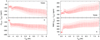 |
Fig. 1 A comparison of predicted planetary transit light curves as a function of stellar effective temperature. Left: average differences between synthetic planetary transit light curves computed using model stellar atmosphere CLIV and using best-fit quadratric limb-darkening laws as a function of effective temperature for the TESS band (top) and K band (bottom). Right: same as the left panels, but for the RMS difference of the light curves. For each effective temperature bin, there are models computed for four different gravities and five different masses. |
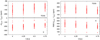 |
Fig. 2 The differences between synthetic planetary transit light curve as a function of stellar gravity. Left: average differences between synthetic planetary transit light curves computed using model stellar atmosphere CLIV and best-fit quadratric limb-darkening laws as a function of stellar gravity for the TESS band (top) and K band (bottom). Right: same as the left panels, but for the RMS difference of the light curves. For each gravity bin, there are models computed for 46 effective temperatures and five different masses. |
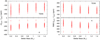 |
Fig. 3 The differences between synthetic planetary transit light curve as a function of stellar mass. Left: average differences between synthetic planetary transit light curves computed using model stellar atmosphere CLIV and using best-fit quadratric limb-darkening laws as a function of stellar mass for the TESS band (top) and K band (bottom). Right: same as the left panels, but for the RMS difference of the light curves. For each mass bin, there are models computed for four different gravities and 46 different effective temperatures. |
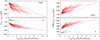 |
Fig. 4 The differences between synthetic planetary transit light curve as a function of stellar atmospheric extension. Left: average differences between synthetic planetary transit light curves computed using model stellar atmosphere CLIV and best-fit quadratric limb-darkening laws as a function of atmospheric extension for the TESS band (top) and K band (bottom). Right: same as the left panels, but featuring the RMS difference of the light curves. Points denoted by black circles are for model stellar atmospheres with Teff ≤ 3700 K. Given the model parameters, there are twenty chains for the atmospheric extension due to the combination of four values of gravity and five values of mass. |
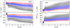 |
Fig. 5 The differences between synthetic planetary transit light curve as a function of stellar effective temperature for different transit inclinations. Left: average differences between synthetic planetary transit light curves computed using model stellar atmosphere CLIV or best-fit quadratric limb-darkening laws as a function of effective temperature for the TESS band (top) and K band (bottom). Right: same as the left panels, but for the RMS of the light curves. The red crosses represent transits with μ0 = 1, blue stars those with μ0 = 0.7, and black open squares those with μ0 = 0.3. The spread of the average differences and RMS values for each μ0 arises from variations in stellar mass and gravity for a given stellar effective temperature. |
5 Limb-darkening law errors as a function of orbital inclination
In this section, we explore how the differences between synthetic planetary transit light curves computed using model stellar atmosphere CLIV and those computed using best-fit limb-darkening coefficients change as a function of orbital inclination. We represent the inclination using μ0, defined in Eq. (4), with an edge-on orbit with μ0 = 1 and a face-on orbit with μ0 = 0. In Paper I, we found that the differences between light curves can increase with increasing inclination until μ0 ≈ 0.3, which corresponds to θ0 ≈ 70°, i ≈ 20° and impact parameter b ≈ 0.95, b ≡ (a/R*) cos i, where a∕R*. is the orbital separation relative to the radius of the star. As a result, for most orbits a change in inclination will lead to greater errors, and the maximum differences between light curves depend on the inclination even more.
We test the role of orbital inclination by first plotting the errors as a function of effective temperature in Fig. 5. The errors due to assuming limb-darkening laws increase as a function of orbital inclination. In the TESS band, the average difference between light curves shifts from about –300 ppm for μ0 = 1, up to –400 ppm for μ0 = 0.7, and up to –600 ppm for μ0 = 0.3. In the K band, the effect is even more significant, with differences up to –700 ppm and –900 ppm for the hottest stars. As such, we are seeing how connected and dependent the light curve and the assumption of limb-darkening laws are to and on each other (Howarth 2011).
The maximum differences also grow as a function of orbital inclination. As μ0 decreases from unity to zero, the maximum difference reaches almost 1700 ppm and 2600 ppm in the TESS and K bands, respectively. Those differences correspond to about 17 and 26% of the surface area of the assumed planet, and hence about 8.5 and 13% of the planet radius for δA = 2δRp. For more inclined orbits, we find errors that are a significant fraction of the relative planet size.
In Fig. 6, we show the effect of atmospheric extension on the difference between the CLIV and the quadratic limb-darkening law. The results are surprising. In Fig. 4, we see that the average and maximum differences between synthetic planet transit light curves grow as a function of atmospheric extension. However, we see that for more inclined orbits the average differences increase rapidly as a function of atmospheric extension. When μ0 = 0.3, we find that the average differences reach almost –600 ppm and –800 ppm in the TESS and K bands, respectively, with an atmospheric extension of ≈2 R⊙/M⊙ (as scaled relatively to the solar effective temperature). This suggests that all stars with planets orbiting in inclined orbits will have significant errors for even smaller atmospheric extensions.
These results place distinct challenges on our understanding of planet transits and secondary effects such as oblateness, rotation, and spots. For instance, for the case of KIC 8462852 (Boyajian et al. 2016) the transits are explained by large families of orbiting comets (or dust clouds; Bodman et al. 2017). Because that analysis ignores limb darkening in fitting the family of comets, if any of the orbits are inclined, the sizes required for the comets will be significantly inaccurate. As such, our results show that we must treat limb darkening in planetary transits with greater care and move from assuming the simple parameterizations to using more realistic models of CLIV.
6 Correcting for limb-darkening law bias in the planetary radius
While the average flux difference offers one measure of the error created by assuming a simple limb-darkening law, it does not offer a significant measurement of biases in the predicted planetary radius. To address this, we started by defining the χ2 from the transit model as
![Mathematical equation: ${\chi ^2} = \sum\limits_z {{{[{f_{{\rm{CLIV}}}}\left({\rho ,z} \right) - {f_{{\rm{LDL}}}}\left({\rho ,z} \right)]}^2}.} $](/articles/aa/full_html/2022/06/aa33635-18/aa33635-18-eq6.png) (6)
(6)
In Eq. (6), z is the projected separation between the center of the planet and the center of the star normalized by the stellar radius. At the edge of the stellar disk, z = 1. This definition offers potential challenges for working with CLIV computed for stellar models with atmospheric extension, which we discuss in Sect. 7. We note this is assuming the small-planet approximation for ease, which will differ slightly from more exact methods. However, this analysis allowed us to probe the order of magnitude of the predicted errors. Because both the CLIV and the best-fit limb-darkening coefficients use the same planet radius and inclination, this χ2 should ideally be a minimum. However, it is possible to ensure improvement by varying some of the parameters. For instance, varying the limb-darkening coefficients changes the predicted stellar flux, which will change the transit depth and, hence, will lead to a different value of the planetary radius. Yet, this change in limb-darkening coefficients will produce compound errors in the way we understand the host star. Similarly, varying the inclination creates biases in the measured limb-darkening coefficients that alter a fit in the same direction. For simplicity, we minimized the χ2 function using just the variation of the planetary radius.
We started by perturbing the radius in the LDL light curve of Eq. (6):
![Mathematical equation: ${\chi ^2} \propto \sum\limits_z {{{[{f_{{\rm{CLIV}}}}\left({\rho ,z} \right) - {f_{{\rm{LDL}}}}\left({\rho + \delta \rho ,z} \right)]}^2}.} $](/articles/aa/full_html/2022/06/aa33635-18/aa33635-18-eq7.png) (7)
(7)
Next, we assumed the small-planet approximation,
 (8)
(8)
is valid for both the CLIV and LDL light curves. In Eq. (8), 4Ω is the stellar flux (and should not be confused with solid angle), and I* is the mean flux blocked by the planet as it transits (Mandel & Agol 2002). For the purpose of this perturbation, we ignore changes in I* as a function of planet radius, as well as second- order changes in δp. Therefore,
![Mathematical equation: $\matrix{{{f_{{\rm{LDL}}}}\left({\rho + \delta \rho ,z} \right)} \hfill & {= 1 - {\rho ^2}{{I*} \over {4\Omega}} - 2{{\delta \rho} \over \rho}{\rho ^2}{{I*} \over {4\Omega}}} \hfill \cr {} \hfill & {= {f_{{\rm{LDL}}}}\left({\rho ,z} \right)2{{\delta \rho} \over \rho}\left[{1 - {f_{{\rm{LDL}}}}\left({\rho ,z} \right)} \right].} \hfill \cr} $](/articles/aa/full_html/2022/06/aa33635-18/aa33635-18-eq9.png) (9)
(9)
We then minimized the χ2-function, Eq. (7), with respect to the radius, obtaining
![Mathematical equation: ${{{\rm{d}}{\chi ^2}} \over {{\rm{d}}\rho}} = 2\sum\limits_z {\left[{{f_{{\rm{CLIV}}}}\left({\rho ,z} \right) - {f_{{\rm{LDL}}}}\left({\rho + \delta \rho ,z} \right)} \right]{{{\rm{d}}{f_{{\rm{LDL}}}}} \over {{\rm{d}}\rho}}} = 0.$](/articles/aa/full_html/2022/06/aa33635-18/aa33635-18-eq10.png) (10)
(10)
Again ignoring changes in I* as a function of p, the derivative of Eq. (8) gives
![Mathematical equation: ${{{\rm{d}}{f_{{\rm{LDL}}}}} \over {{\rm{d}}\rho}} = - 2\rho {{I*} \over {4\Omega}} = - {2 \over \rho}\left[{1 - {f_{{\rm{LDL}}}}\left({\rho ,\;z} \right)} \right].$](/articles/aa/full_html/2022/06/aa33635-18/aa33635-18-eq11.png) (11)
(11)
Using Eqs. (9) and (11) in Eq. (10) gives
![Mathematical equation: $\matrix{{\sum\limits_z {\left\{{\left[{{f_{{\rm{CLIV}}}}\left({\rho ,z} \right) - {f_{{\rm{LDL}}}}\left({\rho ,\;z} \right) + 2{{\delta \rho} \over \rho}\left({1 - {f_{{\rm{LDL}}}}\left({\rho ,z} \right)} \right)} \right]} \right.}} \hfill \cr {\left. {\left[{- {2 \over \rho}\left({1 - {f_{{\rm{LDL}}}}\left({\rho ,\;z} \right)} \right)} \right]} \right\} = 0.} \hfill \cr} $](/articles/aa/full_html/2022/06/aa33635-18/aa33635-18-eq12.png)
Rearranging and solving for δp∕p leads to
![Mathematical equation: ${{\delta \rho} \over \rho} = {{\sum\nolimits_z {\left[{\left({{f_{{\rm{LDL}}}} - {f_{{\rm{CLIV}}}}} \right)\left({1 - {f_{{\rm{LDL}}}}} \right)} \right]}} \over {2\sum\nolimits_z {{{\left({1 - {f_{{\rm{LDL}}}}} \right)}^2}}}}.$](/articles/aa/full_html/2022/06/aa33635-18/aa33635-18-eq13.png) (12)
(12)
This shows again that the average difference in flux offers a rough measure of the error of the fit that affects the predicted depth of the transit and hence the measured planet radius.
We note that Eq. (12) appears to be an explicit function of p since ƒLDL and ƒCLIV themselves also depend on p. However, if we insert Eq. (8) into Eq. (12), then we find that δp∕p is a function of I* ∕4Ω only. The amount of flux blocked by the planet, however, is implicitly dependent on the size of the planet, but to first order Eq. (12) is independent of planet radius. While one could measure these differences using fitting codes, this analysis illustrates how the relative planet radius depends on understanding the limb darkening. Furthermore, we note that this relation implies that the result is independent of stellar radius in that we can replace δp∕p = δrp∕rp.
Figure 7 shows the relative biases to the planet’s radius assuming the quadratic limb-darkening law. This bias is the expected overestimation of the planet radius by fitting methods that assume this limb-darkening law. We plot the difference of the planet’s radius as a function of effective temperature and atmospheric extension. These differences scale with approximately the same behavior as the plots of RMS(ƒcLIv– fLDL). Furthermore, the differences in the planet’s radius are significantly greater than indicated by the average flux difference by almost a factor of twenty in the TESS band and by more than a factor of twenty in the K band. We see again that the bias of the planet’s radius is also greatest for stars with the greatest effective temperature and atmospheric extensions.
As a result, we find that planetary radii can be overestimated by up to 7000 ppm in the near-IR and 5000 ppm in the optical and near-IR TESS bands. This overestimation is small relatively to the assumed size of the planet, especially when the bias is relative to the measured planet size. Assuming the small planet approximation, p = 0.1, and then δp = 500 ppm and 700 ppm in the optical and near-IR, respectively.
The bias for the planetary radius increases with the inclination of the orbit, similarly to that seen for the average flux difference. For instance, Fig. 8 shows that the bias increases by an order of magnitude as μ0 → 0. For the most inclined orbit, and assuming the best-fit limb-darkening coefficients for a quadratic limb-darkening law for each model, the radius bias is about 10% of the actual planet radius for model stellar atmospheres with the greatest atmospheric extension. This bias will be even greater if we assume even simpler limb-darkening laws, such as a linear law or a uniform-disk model (i.e., no limb darkening). Therefore, care must be taken to choose the appropriate limb-darkening parameterization or model when measuring precision values of extrasolar planet radius.
Out of curiosity, we also computed the error in the planetary radius if one assumes a star with no limb darkening, that is, a uniform-disk model. If one uses this method, the planet radius will be underestimated instead of overestimated by about 2 – 5%. This check is consistent with the need for more and more free parameters to precisely measure limb darkening and its impact on the exoplanet radius. However, our analysis and past works highlights the fact that the stellar CLIV cannot be accurately represented by simple functions (Neilson & Lester 2011, 2013a,b).
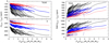 |
Fig. 6 The differences between synthetic planetary transit light curve as a function of stellar atmospheric extension for different transit inclinations. Left: average differences between synthetic planetary transit light curves computed using model stellar atmosphere CLIV or using best-fit quadratic limb-darkening laws as a function of atmospheric extension for the TESS band (top) and K band (bottom). Right: same as the left panels, but for the RMS difference of the light curves. The red crosses represent transits with μ0 = 1, blue stars those with μ0 = 0.3, and black open squares those with μ0 = 0.7. For each inclination, we show twenty chains of atmospheric extension. |
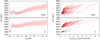 |
Fig. 7 Predicted overestimated value of planetary radius relative to the actual planet size as a function of (left) effective temperature and (right) atmospheric extension for the TESS and K bands for an edge-on orbit. Points denoted by black circles in the right plot are for model stellar atmospheres with Teff ≤ 3700 K. The difference shown here is solely caused by assuming a quadratic limb-darkening law. For the left plot, the spread is due to differences in mass and gravity for a given effective temperature, and for the right-hand plot there are twenty chains caused by the combination of models having four values of gravity and five values of mass. |
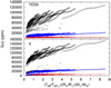 |
Fig. 8 Predicted overestimated value of planetary radius relative to the actual planet size as a function of atmospheric extension for different inclinations in the TESS and K bands. The red crosses represent transits with μ0 = 1, blue stars represent those with μ0 = 0.7, and black open squares represent those with μ0 = 0.3. For each inclination, there are twenty chains of atmospheric extension that resulting from models being computed for four values of gravity and five values of mass. |
7 Atmospheric extension, stellar radius, and transits
The issue of understanding the stellar radius is important not just for planetary transit fits using spherical model atmospheres, but also for fits using plane-parallel models and limb-darkening laws. The geometry of plane-parallel models contains no information about the stellar radius. As such, it is merely assumed that measurements of stellar radii from asteroseismology or stellar evolution models correspond to the stellar radii in planetary transit fits. Similarly, best-fit limb-darkening laws that are based on plane-parallel models or fit directly to observations make the same assumption, and it is unclear whether this is true. Spherically symmetric model stellar atmospheres explicitly contain information about the stellar radius, and therefore about the extension of the atmosphere. Because of the atmospheric extension, the edge of the star is at a physical radius that is not the Rosseland radius. As such, plane-parallel and spherical model stellar atmospheres should not be expected to give the same results when fit to planetary transit or interferometric observations because they make different assumptions about the structure of the photosphere. The challenges for measuring limb darkening and stellar radii (or angular diameters) have been discussed in detail by numerous authors (Wittkowski et al. 2004; Neilson & Lester 2008; Baron et al. 2014; Kervella et al. 2017).
Just as the differences between plane-parallel and spherically symmetric model stellar atmospheres lead to different measurements of stellar radii, they are also fit with varying precision by various limb-darkening laws. Neilson & Lester (2013a,b) showed that six different commonly used limb-darkening laws fit plane-parallel models with much better precision than spherically symmetric models with the same fundamental parameters. The source of this difference is the point of inflection in spherically symmetric CLIV that is a result of including physics of atmospheric extension. Therefore, current limb-darkening laws do not fit the effects of atmospheric extension. This result was found by other works such as Claret & Hauschildt (2003) and Espinoza & Jordán (2016). However, these works avoid the challenge of fitting atmospheric extension by clipping the spherically symmetric model CLIV to remove all information about the extension.
Ligi et al. (2016) found uncertainties in measuring angular diameters of exoplanet host stars to be about 1.9%. This is much greater than the atmospheric extension of these stars. For instance, the Sun has an extension on the order of 0.1% based on the ratio of the pressure scale height in the atmosphere and the solar radius. Therefore, these issues around the definition of stellar radius will not be readily apparent for direct measurements. On the other hand, Mann et al. (2018) measured the relative planet radii for three exoplanets to a precision of δp∣p ≈ 2–4%, while Murgas et al. (2017) reported precisions on the order of 1% and better. Furthermore, the next generation of interferometric observations promises to measure angular diameters to about 0.5% precision (Zhao et al. 2011). At these uncertainties, the biases introduced by assuming the unphysical limb-darkening laws are becoming significant, especially as we attempt to measure spectral properties of exoplanets.
8 Summary
In this work, we took the CLIVs from the Neilson & Lester (2013b) grid of spherically symmetric model stellar atmospheres and the corresponding best-fit limb-darkening coefficients for the quadratic limb-darkening law and computed the differences between synthetic planetary transit light curves using the prescription described by Neilson et al. (2017). We evaluated the error resulting from the use of the limb-darkening laws by computing both the average difference and the greatest difference between the CLIV and LDL transit light curves. These differences were computed as a function of fundamental stellar parameters: effective temperature, gravity, and stellar mass, along with the inclination of the orbit, which we parameterized as μ0 = cos(90º – i).
The results are striking. Before considering the role of inclination, we found that the average differences between CLIV and limb-darkened transit light curves increased as a function of atmospheric extension, which implies that the average differences are greatest for more evolved F-type stars. When inclination is included, the differences increase significantly and depend on the atmospheric extension, indicating the errors are roughly similar for most atmospheric extensions. These negative errors tell us that the relative planetary radii are being overestimated, especially for the F-stars, by as much as 5%, and by at least 1% for an edge-on orbit in the TESS band. Hirano et al. (2016); Fukui et al. (2016) and others report precisions on the order of 1% for measuring Rp∣R*. for planets orbiting F-type stars. Almenara et al. (2015) reported precisions better than 1% for planets orbiting an evolved metal-poor F-star. Given that our models show that Rp∣R* are overestimated, these measurements have a systematic error of at least 1% that is not accounted for in the fits.
We note that these errors are for the ideal situation where one knows the inclination and where the limb-darkening coefficients are the most accurately determined. Our analysis does not consider the cases where inclination, limb-darkening coefficients, and relative radii are fit simultaneously. In those cases, limbdarkening coefficient measurements can deviate significantly from those of model stellar atmospheres (Kipping & Bakos 2011a,b), implying a strong dependence of the limb darkening on other fitting parameters. As the limb-darkening coefficients deviate, so will the errors. This may not change the errors much, but it is something that must be explored in greater detail.
One key conclusion of our work is that we need to measure stellar CLIV both precisely and directly. It is becoming clear that our current assumptions of simple limb-darkening laws are just not good enough for understanding the planetary transit observations. Interferometry is proving to be one method for directly inferring stellar CLIV (Baron et al. 2014; Armstrong et al. 2016; Kervella et al. 2017). We recently showed that we can use interferometric measurements in combination with spectroscopy and spherically symmetric model stellar atmospheres to measure stellar fundamental parameters including stellar masses. That result is based on measurements of atmospheric extension in stars. We suggest that method will be more robust if combined with planetary transit observations as part of a global fit of stellar and planetary parameters. That work and this is part of an ongoing research project to test limb-darkening and stellar radii measurements from interferometric observations against state-of-the-art model stellar atmospheres. However, the results of our current work clearly show that we are reaching the limits of plane-parallel model CLIV and arbitrary limb-darkening laws that have no physics basis.
From this analysis, we predicted biases of the relative radius of an exoplanet δp∣p for a grid of stellar atmosphere models for the wavebands BVRIHK and the TESS bands that are publicly available. While it is preferable to fit the model CLIV to transit light curves and to shift from measuring limb-darkening coefficients to measuring stellar properties, these biases can help improve the precision of planetary transit fits of transit spectra.
Acknowledgements
J.B.L. is grateful for funding from NSERC discovery grants. F.B. acknowledges funding from NSF awards AST-1445935 and AST-1616483. H.R.N. and J.B.L. acknowledge that the University of Toronto operates on traditional land of the Wendat, the Seneca, and most recently, the Mississaugas of the Credit River. The authors are grateful to have the opportunity to work on this land.
References
- Almenara, J. M., Díaz, R. F., Mardling, R., et al. 2015, MNRAS, 453, 2644 [Google Scholar]
- Armstrong, J. T., Baines, E. K., Schmitt, H. R., et al. 2016, Proc. SPIE, 9907, 990702 [NASA ADS] [CrossRef] [Google Scholar]
- Aufdenberg, J. P., Ludwig, H.G., & Kervella, P. 2005, ApJ, 633, 424 [NASA ADS] [CrossRef] [Google Scholar]
- Baron, F., Monnier, J. D., Kiss, L. L., et al. 2014, ApJ, 785, 46 [Google Scholar]
- Baschek, B., Scholz, M., & Wehrse, R. 1991, A&A, 246, 374 [NASA ADS] [Google Scholar]
- Bastien, F. A., Stassun, K. G., Basri, G., & Pepper, J. 2013, Nature, 500, 427 [Google Scholar]
- Bastien, F. A., Stassun, K. G., & Pepper, J. 2014, ApJ, 788, L9 [NASA ADS] [CrossRef] [Google Scholar]
- Bayliss, D., Zhou, G., Penev, K., et al. 2013, AJ, 146, 113 [NASA ADS] [CrossRef] [Google Scholar]
- Bean, J. L., Désert, J.M., Kabath, P., et al. 2011, ApJ, 743, 92 [NASA ADS] [CrossRef] [Google Scholar]
- Berta, Z. K., Charbonneau, D., Désert, J.M., et al. 2012, ApJ, 747, 35 [NASA ADS] [CrossRef] [Google Scholar]
- Bessell, M. S., Brett, J. M., Scholz, M., & Wood, P. R. 1991, A&AS, 89, 335 [NASA ADS] [Google Scholar]
- Bodman, E. H. L., Quillen, A. C., Ansdell, M., et al. 2017, MNRAS, 470, 202 [Google Scholar]
- Boyajian, T. S., LaCourse, D. M., Rappaport, S. A., et al. 2016, MNRAS, 457, 3988 [NASA ADS] [CrossRef] [Google Scholar]
- Cáceres, C., Kabath, P., Hoyer, S., et al. 2014, A&A, 565, A7 [NASA ADS] [CrossRef] [EDP Sciences] [Google Scholar]
- Claret, A. 2000, A&A, 363, 1081 [NASA ADS] [Google Scholar]
- Claret, A. 2017, A&A, 600, A30 [NASA ADS] [CrossRef] [EDP Sciences] [Google Scholar]
- Claret, A., & Hauschildt, P. H. 2003, A&A, 412, 241 [NASA ADS] [CrossRef] [EDP Sciences] [Google Scholar]
- Croll, B., Albert, L., Jayawardhana, R., et al. 2011, ApJ, 736, 78 [NASA ADS] [CrossRef] [Google Scholar]
- Espinoza, N., & Jordán, A. 2016, MNRAS, 457, 3573 [NASA ADS] [CrossRef] [Google Scholar]
- Fukui, A., Narita, N., Kawashima, Y., et al. 2016, ApJ, 819, 27 [NASA ADS] [CrossRef] [Google Scholar]
- Gandolfi, D., Collier Cameron, A., Endl, M., et al. 2012, A&A, 543, L5 [NASA ADS] [CrossRef] [EDP Sciences] [Google Scholar]
- Gillon, M., Demory, B.O., Madhusudhan, N., et al. 2014, A&A, 563, A21 [NASA ADS] [CrossRef] [EDP Sciences] [Google Scholar]
- Hirano, T., Fukui, A., Mann, A. W., et al. 2016, ApJ, 820, 41 [Google Scholar]
- Howarth, I. D. 2011, MNRAS, 418, 1165 [NASA ADS] [CrossRef] [Google Scholar]
- Huang, C. X., Hartman, J. D., Bakos, G. Á., et al. 2015, AJ, 150, 85 [NASA ADS] [CrossRef] [Google Scholar]
- Kervella, P., Bigot, L., Gallenne, A., & Thévenin, F. 2017, A&A, 597, A137 [NASA ADS] [CrossRef] [EDP Sciences] [Google Scholar]
- Kipping, D., & Bakos, G. 2011a, ApJ, 730, 50 [NASA ADS] [CrossRef] [Google Scholar]
- Kipping, D., & Bakos, G. 2011b, ApJ, 733, 36 [NASA ADS] [CrossRef] [Google Scholar]
- Lester, J. B., & Neilson, H. R. 2008, A&A, 491, 633 [NASA ADS] [CrossRef] [EDP Sciences] [Google Scholar]
- Ligi, R., Creevey, O., Mourard, D., et al. 2016, A&A, 586, A94 [NASA ADS] [CrossRef] [EDP Sciences] [Google Scholar]
- Mandel, K., & Agol, E. 2002, ApJ, 580, L171 [Google Scholar]
- Mann, A. W., Vanderburg, A., Rizzuto, A. C., et al. 2018, AJ, 155, 4 [Google Scholar]
- Morello, G., Tsiaras, A., Howarth, I. D., & Homeier, D. 2017, AJ, 154, 111 [NASA ADS] [CrossRef] [Google Scholar]
- Murgas, F., Pallé, E., Parviainen, H., et al. 2017, A&A, 605, A114 [NASA ADS] [CrossRef] [EDP Sciences] [Google Scholar]
- Neilson, H. R., & Lester, J. B. 2008, A&A, 490, 807 [NASA ADS] [CrossRef] [EDP Sciences] [Google Scholar]
- Neilson, H. R., & Lester, J. B. 2011, A&A, 530, A65 [NASA ADS] [CrossRef] [EDP Sciences] [Google Scholar]
- Neilson, H. R., & Lester, J. B. 2013a, A&A, 554, A98 [CrossRef] [EDP Sciences] [Google Scholar]
- Neilson, H. R., & Lester, J. B. 2013b, A&A, 556, A86 [CrossRef] [EDP Sciences] [Google Scholar]
- Neilson, H. R., Baron, F., Norris, R., Kloppenborg, B., & Lester, J. B. 2016, ApJ, 830, 103 [NASA ADS] [CrossRef] [Google Scholar]
- Neilson, H. R., McNeil, J. T., Ignace, R., & Lester, J. B. 2017, ApJ, 845, 65 [NASA ADS] [CrossRef] [Google Scholar]
- Rauer, H., Catala, C., Aerts, C., et al. 2014, Exp. Astron., 38, 249 [Google Scholar]
- Ricker, G. R., Winn, J. N., Vanderspek, R., et al. 2015, J. Astron. Teles. Instrum., Syst., 1, 014003 [Google Scholar]
- Ricker, G. R., Vanderspek, R., Winn, J., et al. 2016, SPIE Conf. Ser., 9904, 99042B [NASA ADS] [Google Scholar]
- Seager, S., & Deming, D. 2010, ARA&A, 48, 631 [NASA ADS] [CrossRef] [Google Scholar]
- Sing, D. K. 2010, A&A, 510, A21 [NASA ADS] [CrossRef] [EDP Sciences] [Google Scholar]
- Smalley, B., Anderson, D. R., Collier-Cameron, A., et al. 2012, A&A, 547, A61 [NASA ADS] [CrossRef] [EDP Sciences] [Google Scholar]
- Wittkowski, M., Aufdenberg, J. P., & Kervella, P. 2004, A&A, 413, 711 [NASA ADS] [CrossRef] [EDP Sciences] [Google Scholar]
- Zhao, M., Monnier, J. D., Che, X., et al. 2011, PASP, 123, 964 [NASA ADS] [CrossRef] [Google Scholar]
All Figures
|
Fig. 1 A comparison of predicted planetary transit light curves as a function of stellar effective temperature. Left: average differences between synthetic planetary transit light curves computed using model stellar atmosphere CLIV and using best-fit quadratric limb-darkening laws as a function of effective temperature for the TESS band (top) and K band (bottom). Right: same as the left panels, but for the RMS difference of the light curves. For each effective temperature bin, there are models computed for four different gravities and five different masses. |
| In the text | |
|
Fig. 2 The differences between synthetic planetary transit light curve as a function of stellar gravity. Left: average differences between synthetic planetary transit light curves computed using model stellar atmosphere CLIV and best-fit quadratric limb-darkening laws as a function of stellar gravity for the TESS band (top) and K band (bottom). Right: same as the left panels, but for the RMS difference of the light curves. For each gravity bin, there are models computed for 46 effective temperatures and five different masses. |
| In the text | |
|
Fig. 3 The differences between synthetic planetary transit light curve as a function of stellar mass. Left: average differences between synthetic planetary transit light curves computed using model stellar atmosphere CLIV and using best-fit quadratric limb-darkening laws as a function of stellar mass for the TESS band (top) and K band (bottom). Right: same as the left panels, but for the RMS difference of the light curves. For each mass bin, there are models computed for four different gravities and 46 different effective temperatures. |
| In the text | |
|
Fig. 4 The differences between synthetic planetary transit light curve as a function of stellar atmospheric extension. Left: average differences between synthetic planetary transit light curves computed using model stellar atmosphere CLIV and best-fit quadratric limb-darkening laws as a function of atmospheric extension for the TESS band (top) and K band (bottom). Right: same as the left panels, but featuring the RMS difference of the light curves. Points denoted by black circles are for model stellar atmospheres with Teff ≤ 3700 K. Given the model parameters, there are twenty chains for the atmospheric extension due to the combination of four values of gravity and five values of mass. |
| In the text | |
|
Fig. 5 The differences between synthetic planetary transit light curve as a function of stellar effective temperature for different transit inclinations. Left: average differences between synthetic planetary transit light curves computed using model stellar atmosphere CLIV or best-fit quadratric limb-darkening laws as a function of effective temperature for the TESS band (top) and K band (bottom). Right: same as the left panels, but for the RMS of the light curves. The red crosses represent transits with μ0 = 1, blue stars those with μ0 = 0.7, and black open squares those with μ0 = 0.3. The spread of the average differences and RMS values for each μ0 arises from variations in stellar mass and gravity for a given stellar effective temperature. |
| In the text | |
|
Fig. 6 The differences between synthetic planetary transit light curve as a function of stellar atmospheric extension for different transit inclinations. Left: average differences between synthetic planetary transit light curves computed using model stellar atmosphere CLIV or using best-fit quadratic limb-darkening laws as a function of atmospheric extension for the TESS band (top) and K band (bottom). Right: same as the left panels, but for the RMS difference of the light curves. The red crosses represent transits with μ0 = 1, blue stars those with μ0 = 0.3, and black open squares those with μ0 = 0.7. For each inclination, we show twenty chains of atmospheric extension. |
| In the text | |
|
Fig. 7 Predicted overestimated value of planetary radius relative to the actual planet size as a function of (left) effective temperature and (right) atmospheric extension for the TESS and K bands for an edge-on orbit. Points denoted by black circles in the right plot are for model stellar atmospheres with Teff ≤ 3700 K. The difference shown here is solely caused by assuming a quadratic limb-darkening law. For the left plot, the spread is due to differences in mass and gravity for a given effective temperature, and for the right-hand plot there are twenty chains caused by the combination of models having four values of gravity and five values of mass. |
| In the text | |
|
Fig. 8 Predicted overestimated value of planetary radius relative to the actual planet size as a function of atmospheric extension for different inclinations in the TESS and K bands. The red crosses represent transits with μ0 = 1, blue stars represent those with μ0 = 0.7, and black open squares represent those with μ0 = 0.3. For each inclination, there are twenty chains of atmospheric extension that resulting from models being computed for four values of gravity and five values of mass. |
| In the text | |
Current usage metrics show cumulative count of Article Views (full-text article views including HTML views, PDF and ePub downloads, according to the available data) and Abstracts Views on Vision4Press platform.
Data correspond to usage on the plateform after 2015. The current usage metrics is available 48-96 hours after online publication and is updated daily on week days.
Initial download of the metrics may take a while.