| Issue |
A&A
Volume 661, May 2022
|
|
|---|---|---|
| Article Number | A88 | |
| Number of page(s) | 15 | |
| Section | Galactic structure, stellar clusters and populations | |
| DOI | https://doi.org/10.1051/0004-6361/202142876 | |
| Published online | 05 May 2022 | |
The nature of the X-ray sources constituting the 6.7 keV Galactic ridge emission
Hamburger Sternwarte, Universität Hamburg, Gojenbergsweg 112, 21029 Hamburg, Germany
e-mail: jschmitt@hs.uni-hamburg.de
Received:
10
December
2021
Accepted:
14
January
2022
We reanalyze the deep Chandra X-ray observations near the Galactic center and show that reliable identifications of X-ray sources can be obtained with the Gaia EDR3 data to investigate which types of stellar sources are responsible for the X-ray emission observed from the Galactic ridge (GRXE). In the central 3 arcmin region 318 X-ray sources are detected, about one-third of which can be identified with objects listed in Gaia EDR3; however, only 22 objects have parallaxes and colors and can be placed into a color-magnitude diagram and thus be identified as coronal X-ray emitters. A rather large fraction of the X-ray sources cannot be identified with Gaia EDR3 entries, and we discuss the optical brightnesses of these sources. We analyze the counting events obtained in the 6.7 keV iron line spectral region and show that they are mainly caused by background events; however, 237 events can be associated with the detected X-ray sources, and we carry out an intensity measurement of the whole iron line complex. Our analysis shows that the mean energy of this iron line complex is located at a wavelength of ≈1.87 Å, where a variety of emission lines of iron ions in ionization stages FeXXIII–FeXXV are located; another line at 7.0 keV is only marginally detected, while the fluorescent 6.4 keV neutral iron line is clearly not seen. We demonstrate that only a few of the detected X-ray sources are responsible for the bulk of the observed iron line emission. We discuss to what extent coronal emission can be held responsible and demonstrate that M dwarfs and active binary systems like RS CVn systems do not significantly contribute to the observed emission; instead, it appears that the Galactic ridge emission is produced by optically fainter sources. Among the known population of cataclysmic variables, polars and dwarf novae appear to be the most promising candidates as main contributors to the GRXE.
Key words: stars: activity / stars: coronae / X-rays: diffuse background
© ESO 2022
1. Introduction
The physical origin of the X-ray emission observed along the Galactic ridge (GRXE) is still unclear, even almost 40 years after its discovery by Worrall et al. (1982) in HEAO A2 data. The ridge emission can be observed over more than half of the disk of the Galaxy, reaching an intensity peak near the Galactic center (Revnivtsev et al. 2006). The observed ridge emission is quite hard, and at energies above 2 keV, where absorption effects from the interstellar medium are less relevant, the spectrum of the GRXE is consistent with that of a plasma in collisional equilibrium, with the presence of an iron line at 6.7 keV (cf. Revnivtsev et al. 2006) indicating rather plasma high temperatures.
The origin of the GXRE emission has been discussed as truly diffuse emission from a rather hot plasma (cf. Ebisawa et al. 2001) or as a superposition of the emission from many point-like sources (cf. Worrall & Marshall 1983; Revnivtsev et al. 2009). The major difficulty with the former ansatz is the problem of plasma confinement: the gravitational potential of the Milky Way is too small to prevent the plasma from escaping, and hence other confining mechanisms or a persistent source of new plasma are needed. With the latter ansatz, the confinement problem is solved; however, the questions are then which population of Galactic X-ray sources is responsible for the GRXE and does this population also exist in the solar neighborhood.
For various reasons an origin of a significant fraction and possibly all of the GRXE from unresolved point sources appears very likely. In particular, Revnivtsev et al. (2006) demonstrated that the observed GRXE correlates very well with the infrared brightness distribution of the Galaxy, which in turn correlates well with the underlying stellar densities. Furthermore, using a very deep Chandra pointing near the Galactic center, Revnivtsev et al. (2009) were able to resolve more than 80% of the observed diffuse X-ray emission when concentrating on the inner core region of the Chandra field where the instrumental point response function is sharpest. The resolved sources show, in aggregate, the previously observed 6.7 keV iron line complex; however, an optical identification of the X-ray sources was not possible at the time due to the faintness and crowding of the optical counterparts; Revnivtsev et al. (2009) merely write that “most of the sources ... are probably accreting white dwarfs and binary stars with strong coronal activity”. Other types of X-ray sources may also contribute to the GRXE; for example, Molaro et al. (2014) argue that a significant fraction of the GRXE is caused by scattering of the X-ray flux of bright X-ray binaries off interstellar dust grains.
A very detailed reanalysis of the deep Chandra pointing data near the Galactic center, first presented by Revnivtsev et al. (2009), was carried out by Hong (2012); in particular, Hong (2012) studies the influence of various detection algorithms and the chosen parameter settings on the resulting X-ray source lists. While Hong (2012) finds that the faintest ≈120 sources of the 473 sources reported by Revnivtsev et al. (2009) are probably not real, the main results obtained by Revnivtsev et al. (2009) are confirmed by and large, yet at the same time Hong (2012) argues (without having access to any optical identifications) that the resolved hard X-ray flux above 3 keV is dominated by rather bright, hard X-ray sources such as magnetic cataclysmic variables and not by coronal X-ray sources.
Morihana et al. (2013) analyzed the spectral properties of the X-ray sources detected in the deep Chandra pointing in detail. For the brighter sources these authors perform detailed spectral modeling, while the spectral properties of the bulk of the fainter sources are analyzed in an X-ray color-color diagram (see Sect. 3.2 for details). In this X-ray color-color diagram Morihana et al. (2013) identify three different regions, which they speculate are populated by different types of astrophysical sources; based on spectral fits (rather than optical identifications, for example) to composite X-ray spectra, Morihana et al. (2013) argue that these populations belong to active galactic nuclei and accreting white dwarfs, and to active stars with and without the 6.7 keV iron line emission.
In the meantime an extremely valuable data source in the form of the Gaia catalog has become available. The Gaia mission (for further discussion see Sect. 2.2 and references therein) provides precise positions and parallaxes for more than a billion objects down to a magnitude limit below g ≈ 20, and therefore it well behooves us to examine which of the X-ray sources in the core region of the Chandra field can be identified with Gaia entries and what consequences can be drawn on the nature of these counterparts.
As discussed in some detail by Schmitt et al. (2022), one expects coronal X-ray emitters to obey the so-called saturation limit of LX/Lbol ≈ 10−3; in other words, for coronal sources the observed X-ray flux is at most about one-thousandth of the bolometric flux; this saturation limit is first clearly described for X-ray sources by Fleming et al. (1993), and for a review we refer to Güdel (2004). No truly convincing physical explanation of this saturation limit is known; in addition, some scatter is observed around the nominal value of 10−3; however, at least outside flares, no strong violations of this limit are known in simultaneous observations. As a consequence of this saturation limit, a limiting optical magnitude exists for all X-ray sources that are purely coronal emitters, and hence it is worthwhile to utilize the information contained in the Gaia catalog to determine the nature of the X-ray sources detected in the Chandra deep field.
The plan of our paper is as follows. We first describe in Sect. 2 the database used for our efforts. In Sect. 3 we discuss the problem of (de-)reddening, the determination of optical and X-ray fluxes, a parameter-free characterization of the Chandra X-ray spectra, the conversion of X-ray count rates to X-ray fluxes, the spatial distribution of the Gaia and Chandra sources, the completeness of the Gaia data in the relevant sky area, the positional match between the two data sets, and the expected level of contamination. In Sect. 4 we present our results in terms of the apparent magnitude distribution of the Gaia counterparts, the de-reddened color-magnitude diagram. We discuss the optical and X-ray properties of the matched sources and analyze the observed 6.7 keV emission in detail and develop a statistical method for associating the observed iron line signal with the detected X-ray sources. In Sect. 5 we we present a discussion of the implications of our findings, and in Sect. 6 we present our conclusions.
2. Observations
2.1. Chandra data
For our study of the X-ray source population we use the 2.0 version of the Chandra source catalog (CSC), which the Chandra project considers to be the most complete catalog of X-ray sources detected by the Chandra X-ray Observatory; for a detailed description of this catalog and the procedures employed in its construction we refer to Evans et al. (2010). One major improvement made in CSC 2.0 (compared to previous releases) is the use of combined (i.e., overlapping) Chandra observations for detecting X-ray sources. With this new feature of the catalog, observations with similar aim points are stacked, and in this fashion considerably higher sensitivities for detecting fainter sources are achieved.
We specifically used the CSC 2.0 version released in 2019 and made available through the Centre de Données astronomiques de Strasbourg (CDS). With the position RA = 17h 51m 26s and δ = −29° 35′ 11″, corresponding to l = 0.097° and b = −0.142°, as a reference point, we retrieve a total of 318 sources within 3 arcmin of that position if we focus on sources with positional errors below 0.5 arcsec, which is necessary for reliable identifications in this crowded region. In the following we refer to this region as our Chandra core region.
From the Chandra X-ray data center we also downloaded the data for the observation sequence 900837, which is divided into a number of portions with the ObsIDs 5934, 6362, 6365, 9500–9505, 9854, 9855, 9892, and 9893, and is the data used by Revnivtsev et al. (2009) in their deep GRXE study. The nominal aim points of these observations are very similar, and we used again the position RA = 17h 51m 26s and δ = −29° 35′ 11″ as a reference point. We obtained the Chandra pipeline produced photon event files and merged the individual ObsIDs by computing the right ascension and declination for each registered counting event. We note in passing that all X-ray data were taken with the Advanced CCD Imaging Spectrometer-I (ACIS-I), a detailed description of which is given by Garmire et al. (2003). Briefly, the ACIS-I instrument covers the energy range 0.3−8.0 keV with a typical spectral resolution of about 200 eV; however, this depends somewhat on the source position on the X-ray detector.
2.2. Gaia data
The Gaia mission, launched in December 2013, is an ESA large mission devoted to the precise measurement of positions, magnitudes, distances, and space velocities of more than a billion stars; a detailed description of the Gaia hardware, its scientific goals, and in-orbit performance is given by the Gaia Collaboration (2016). To date, the Gaia project has released data in three steps: Gaia DR1 in 2016, Gaia DR2 in 2018, and an (early) release Gaia EDR3 in 2020; further data releases are planned in the coming years. Gaia EDR3 contains positions, proper motions, and parallaxes for about 1.468 × 10⁹ sources, and for the purposes of this paper, we work with the Gaia EDR3 data release.
We downloaded all of the Gaia EDR3 data centered on our chosen reference position to cover the whole Chandra field. In our Chandra core region we find a total of 9682 Gaia entries, corresponding to a source density of more than 1.2 × 10⁶ sources per square degree; we note that this census is not complete and refer to Sect. 4.3 for more detailed discussion of this issue. Of the total number of entries, 9606 sources have a g magnitude, but only 4485 have a Gaia measured BP − RP color, which is necessary for an assessment of the nature of the counterpart, and only 793 sources have measured parallaxes with a S/N in excess of 3. Thus, unfortunately, only a very small fraction of the Gaia population in the Chandra core region can be meaningfully placed in a color-magnitude diagram (CMD). We note in passing that Gaia also provides proper motions, but for the vast majority of sources the proper motion corrections from the Gaia epoch to that of the Chandra observations is well below the typical position errors of the X-ray sources.
3. Data analysis
3.1. Reddening and dereddening
Clearly, absorption and the ensuing reddening play an important role in any deep X-ray study at low galactic latitudes. Inspecting the spectral fitting results obtained by Morihana et al. (2013), we find derived column density values of log(NH) between 21.6 and 22.4 (see their Tables 2 and 3). Using the canonical relations AV = 3.1 × EB − V and NH = 5.3 × 1021 cm−2 × EB − V (Predehl & Schmitt 1995), relating visual absorption AV, color excess EB − V and hydrogen column density NH, this corresponds to AV values between 2.3 and 14.2.
Andrae et al. (2018) study absorption and color excess in Gaia data, and from model atmospheres these authors expect the approximate relation AG ∼ 2 × EBP − RP between the absorption AG in the GaiaG band and the Gaia color excess EBP − RP; however, a direct determination of AG from Gaia data alone is quite difficult since decreasing effective temperature and increasing absorption both lead to reddening, and it is hard to disentangle the two effects. A scatter plot between AV and AG (see Fig. 16 in Andrae et al. 2018) does not show any clear correlations, and Andrae et al. (2018) find AV ∼ AG with quite a bit of scatter (see their Table 6). For cool stars with effective temperatures in the range 5000 K–6000 K perhaps suggests AV ∼ 1.5 AG with again considerable uncertainty. Taking this value would lead to estimates of AG between 1.5 and 9.5 for the X-ray sources in the core region, with the bulk of the sources being located at the lower values; we return to this issue in Sect. 3.2.2.
3.2. Determination of X-ray and optical fluxes
A physical interpretation of the X-ray data can only be obtained from X-ray fluxes. For the stronger sources, X-ray fluxes can be derived from spectral modeling; for the weaker sources, spectral modeling often yields ambiguous results and different methods should be used. Morihana et al. (2013) present detailed spectral X-ray modeling for ten X-ray sources with more than 1000 registered counts (in their Tables 3 and 4) and find that two sources have thermal spectra, while the remaining eight spectra have a nonthermal origin; unfortunately, none of these sources are located in the Chandra core region.
X-ray fluxes are also provided in the CSC catalog offered through CDS; however, the CSC catalog does not provide the actual source count rates, but only inferred energy fluxes, which in turn depend on a spectral model chosen for the flux derivation. In the case of CSC, this model is a power law which is inappropriate for thermal sources, which the coronal emitters ought to be. Furthermore, in a number of cases no valid flux values are given in the CSC catalog, although visual inspection clearly shows the presence of an X-ray source at the respective position. Therefore, in an attempt to derive consistent results, we obtained our own count rate measurements from the merged photon data set; as a sanity check we compared our rates with those derived by Morihana et al. (2013). From their Table 2 we can recover 90% of the sources in the core region and the derived count rates agree to within the errors in 99% of the cases. These count rates are then used for flux inference, as described below.
3.2.1. Parameter-free chracterization of X-ray spectra
The energy range covered by ACIS-I is rather broad, and thus a spectral characterization of the incident photon flux is highly desirable. Morihana et al. (2013) use a statistical description of the X-ray spectra: for every X-ray source the cumulative distribution of the energies of the individual photon events is calculated and the quartiles E25, E50, and E75 are determined, denoting those energies within which 25%, 50%, and 75% of the registered events are contained. These quartiles are then normalized with the expression
and choosing Emin = 0.5 keV and Emax = 8 keV, Morihana et al. (2013) construct the dimensionless quantities
and

to characterize the cumulative event distribution. Here q1 is a measure of the median photon energy, while q2 describes the skewness of the spectrum; for a flat spectrum (in observed count space, not in incident flux space) q1 = 0 and q2 = 1 is obtained. Values of q1 > 1 indicate mean photon energies in excess of 4.25 keV, and values of q2 > 1 indicate soft spectra. We use this scheme in Sect. 4 to characterize the properties of the X-ray sources depending on their classification.
3.2.2. X-ray energy conversion factors
At some point we need to convert the measured X-ray count rates into physical energy fluxes. In the absence of a physical model for the incident X-ray flux, this is a nontrivial problem, at least for sources with poor counting statistics. For purposes of illustration, we consider a source with flat incident energy flux density observed at, say, 1 keV and 7 keV. The incident photon flux density then differs by a factor of 7, and since the effective areas of most X-ray facilities are much smaller at 7 keV than at 1 keV, say by a factor of 5, the observed count rate at 7 keV would be 35 times lower than that at 1 keV, yet the incident energy flux is the same by construction. As a consequence, the noise of the flux measurement at 7 keV would be much larger and would in fact dominate the overall error budget. Conversely, if the flatness of the incident X-ray spectrum were known, it would be possible to measure the flux at 1 keV, where the noise is much lower, and to use the spectral model to extrapolate to the total flux.
For these reasons, instead of using the median photon energy, which is normally different for every source considered, as done by Morihana et al. (2013), we prefer to use the classical approach of using energy conversion factors (ECFs) to convert from count rate to energy flux. Since we specifically want to investigate to what extent active stars are producing GXRE, we consider emission from plasma in collisional equilibrium and used the WebPIMMS facility at the Chandra website to compute the resulting count rates for a sequence of input spectra; our results are listed in Table 1.
Energy conversion factors (absorbed and unabsorbed), X-ray and G band absorptions, and attentuation ratios in the optical and X-ray band for various values of interstellar absorption column densities.
We specifically assumed log T = 7.3 and solar abundances and considered interstellar absorption densities in the range from 1.5 × 1021 cm−2 to 12 × 1021 cm−2, which is the range of absorption values found by Morihana et al. (2013) in their spectral analysis of strong sources. We considered the conversion from the observed ACIS-I count rate in the 0.5−7 keV band into the 0.2−2.3 keV band both for the absorbed and unabsorbed fluxes. The use of the 0.2−2.3 keV band appears odd, yet we wish to compare our results to values obtained from eROSITA, which are quoted in this energy band. Interestingly, the ECFs for the absorbed fluxes change very little (< 20%) and decrease with increasing column, an effect due to the chosen band pass, which loses more and more flux with increasing absorption. Therefore, the errors committed by using a constant ECF are moderate, but only if the model assumptions are correct. However, the unabsorbed ECFs increase as expected since the mean energy of each registered photon increases with increasing NH, thus more and more X-ray flux is lost. To ease the comparison with optical absorption values, we quote the relative absorption in terms of an X-ray absorption AX, defined through
Finally, we convert the assumed values of NH into AG using the formulae provided in Sect. 3.1. All resulting values are listed in Table 1, where we also provide the ratio of the attenuations in the optical to those in the X-ray band. As is apparent from Table 1, the X-ray range is surprisingly less attenuated than the G band, yet we must keep in mind that this is a consequence of the chosen X-ray spectrum: the emission spectrum of a collisional plasma with a temperature of log T = 7.3 extends to higher energies where the absorption is low. Had we chosen a lower, solar-like X-ray temperature, the situation would be different, but such plasmas do not produce significant iron line emission at 6.7 keV.
In their study of the so-called eFEDS-field observed by eROSITA, Schneider et al. (2022) obtained a complete identification of its stellar content and derived the fX/fg distribution for more than 2000 stellar X-ray sources with a limiting flux of about 1 × 10⁻¹⁴ erg s−1 cm−2. As shown by Schneider et al. (2022), the most likely values of log(fX/fg) are attained around values of ≈−3, a few sources extend up to −2, and the number of coronal sources with fX/fg > 10−2 is extremely small. According to Schneider et al. (2022) these sources are typically quite red, so that the peak in their flux distribution is redward of the GaiaG band pass. The eFEDS field is located at moderate galactic latitudes (b ≈ 30°), and the absorption values for Galactic sources also ought to be moderate. Therefore, the log(fX/fg) values derived by Schneider et al. (2022) represent essentially the intrinsic values without absorption, while the values we derived for the Chandra core region can easily be affected by differential absorption between the X-ray and optical band. The last column in Table 1 therefore provides the correction factors by which the observed values need to be divided to be comparable to the results of Schneider et al. (2022), and it becomes clear that for moderate NH values below 6 × 1021 cm2 our conclusions from Sect. 3.2.3 are not significantly affected.
3.2.3. Optical energy conversion factor and limiting magnitudes for coronal sources
The Gaia catalog lists an apparent magnitude for the Gaia band denoted by g. Since we want to compare the recorded fluxes in the optical and X-ray range, we also need to convert the Gaia derived magnitude to a physical flux, which we achieve with the formula1

Motivated by the results of Schneider et al. (2022), we then write

and combine Eqs. (5) and (6) to obtain, assuming a limiting flux of 10−16 erg s−1 cm−2 for the Chandra core region, an expression for the faintest possible stellar magnitude glim through glim ≈ 27.5 − 2 × α. For sources with α = 4 we find, glim ≈ 17.5, for α = 3, glim ≈ 20, and for α = 2, glim ≈ 22.5. Comparing these numbers with the results shown in Fig. 3, we conclude that the bulk of the normal (i.e., nondegenerate) stellar X-ray population should be contained in Gaia EDR3 with parallax information, and only some of the red active M dwarfs will have apparent magnitudes below the Gaia cutoff.
4. Results
4.1. Positional match between the Chandra and Gaia sources
We now match the catalogued 318 Chandra sources in the Chandra core region with the Gaia EDR3 sources. Carrying out a positional match with all of the Gaia EDR3 entries in this area, we can compute the nearest neighbor distribution (NND) between Chandra X-ray sources and Gaia entries, plotted in Fig. 1. The distribution is clearly bimodal; the orange hump must represent the true matches, while the much broader green curve represents physically unrelated random matches. For a random distribution of 2D data points with surface density η, the probability pNN(r) to find the nearest neighbor with respect to to a randomly chosen reference position at distance r can be analytically calculated through
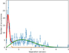 |
Fig. 1. Nearest neighbor distribution between the X-ray sources in the Chandra core region and the Gaia entries. The yellow curve denotes a fit of a Rayleigh distribution to the true matches, the nearest neighbor distribution to the random matches is shown in green, and the summed curve in red; see text for details. |
The distance distribution between Gaia entries and X-ray sources is modeled with a Rayleigh distribution through
with the parameter σ describing the match distance dispersion; the expressions Eqs. (7) and (8) become mathematically equivalent by setting  .
.
As is clear from Fig. 1, the observed nearest neighbor distribution (blue data points in Fig. 1) can be well modeled as the sum of a Rayleigh distribution (yellow curve in Fig. 1) and a NND (green curve in Fig. 1); the determined best fit dispersion of the Rayleigh distribution was found as σ = 0.14 arcsec, the best fit surface density is η = 1.33 × 10⁶ deg−2. The latter value corresponds to a mean distance of 1.55 arcsec between two entries (i.e., an order of magnitude larger than the typical error). To make reliable identifications based on positional coincidence it is clearly of utmost importance to have positional accuracies well below 1 arcsec, and furthermore some level of contamination in the sense that unrelated Gaia entries are close to Chandra X-ray sources (albeit accidentally) and are hence erroneously identified, is unavoidable even at that level. Specifically, we find 98 ± 5 sources contained in the narrow peak in Fig. 1 (i.e., only about 30% of the X-ray sources) have Gaia listed counterparts. The Gaia magnitude limit is well defined at a magnitude g ≈ 20.5 (see Fig. 3, discussed below); however, due to the extremely high potential counterpart densities in the Chandra deep field, significant incompleteness effects (discussed in detail in Sect. 4.3) set in already at brighter magnitudes.
In Table A.1 we provide a list of all Chandra sources that can be matched to Gaia with a geometric association probability of at least 10%; in Table A.1 we purposely include identifications with rather low probability to demonstrate that the derived sample is quite insensitive to the precise cutoff value chosen. Focusing on the 98 most likely identifications, only 51 of them have Gaia color information, which allows an assessment of the spectral type, and only 21 of them have color and parallax information, which allows placement in a CMD. A total of 26 out of 98 counterparts are brighter than 18 mag, and, as we explain in Sect. 4.3, this number should be accurate; 72 out of 98 counterparts are fainter than 18 mag, and this group of objects may be affected by (in-)completeness effects. Table A.1 contains three objects flagged as “Star” with association probabilities below our chosen cutoff (0.72), while 31 objects are accepted stars, yet not all objects recognized as stars have valid BP − RP colors and can therefore not be placed into a CMD; one object (Gaia EDR3 4056468075694237824) surprisingly has no BP − RP color despite its large brightness, we are therefore left with only 22 objects with known parallax and color, which are required for a placement in a CMD.
4.2. Contamination
A crucial question in all identification efforts is the question of contamination; in other words, how many of the identified sources are caused by random matches without any physical association. From the derived NND (see Fig. 1) we can immediately compute the (purely geometric) probability for a true association versus match distance and can then derive for each of the 318 Chandra sources the (geometrical) probability passoc to be associated with the nearest Gaia neighbor. The resulting distribution is highly bimodal with most of the values near zero (no match) or unity (match). The summed probability is 97.5; if we then take those 98 sources with the smallest matching distances as correctly identified, we find a limiting passoc-value of 0.75. With this choice of cutoff we expect 6.8 random identifications, meaning that the reliability of our identifications is expected to be at around the 7% level.
4.3. Completeness
The Gaia EDR3 catalog is known to be incomplete both at the bright and faint end; for a detailed discussion of the general catalog properties and especially its completeness properties we refer to Fabricius et al. (2021). As discussed by Fabricius et al. (2021), in a crowded field like the Chandra core region, the EDR3 catalog does not reach its nominal magnitude limit of ∼20.5. Due to a finite mass memory and telemetry limit of the Gaia hardware, the number of simultaneously observable stars is limited and, as a consequence, in a crowded field fainter stars will start dropping out and not be transmitted to the ground and hence are missing in the catalog. We can demonstrate this effect in the Chandra core region by investigating the object number versus g magnitude diagram, shown in Fig. 2, where we plot the observed log N–log S-curve (blue data points). At g ≈ 18.5, the number count curve becomes flat due to the finite mass memory and telemetry, while the cutoff near g ≈ 20.5 is instrumental. Because of this effect we are missing sources in the magnitude range 18.5 < g < 20.5 (i.e., the region between the red and blue curves in Fig. 2). If we approximate the actual log N–log S-curve with an exponential law (a realization of which is shown with the red data points in Fig. 2), we can estimate the number of the missing sources. In the specific case shown in Fig. 2, more than 26 000 sources would actually be missed. This is large; however, by construction the vast majority of the missed sources are fainter than g = 20, and only around 6000 of the missed sources are brighter than g = 20. We thus conclude that incompleteness is negligible for sources brighter than 18.5 and between 50 and 100% in the range 18.5 < g < 20.5.
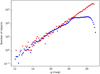 |
Fig. 2. Number of objects vs. g-magnitude for all Gaia entries in the Chandra core region (blue data points); the red data points show a hypothetical Chandra core region log N–log S curve without any incompleteness effects; see text for more details. |
4.4. Apparent color-magnitude distribution of the Gaia sources
To obtain an overview of the properties of the Gaia sources, we show an observed (i.e., reddened) color-magnitude diagram of 4184 Gaia entries located in the Chandra core region in Fig. 3, for which measurements of magnitude and color are available, meaning that we plot apparent magnitude versus observed color. We note that there are a few entries outside the shown plotting range, but the vast majority of sources are located inside the chosen plotting window. In Fig. 3 the blue data points denote those objects for which a parallax measurement with S/N > 3 is available, while for the red objects no parallax and distance information is available in Gaia EDR3. Figure 3 shows that parallaxes are available for objects brighter than about 18 mag and bluer than BP − RP ∼ 3, and most of the fainter or redder objects have no Gaia parallax measurements. Overall, 739 objects corresponding to 12% of the population have significant parallax measurements.
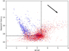 |
Fig. 3. Observed color-magnitude diagram for Gaia entries in the Chandra core region. The blue data points have parallax measurements with S/N > 3, the red data points do not. The black arrow indicates the reddening vector; the region in the upper left is where Gaia EDR3 is complete and where proper stars ought to be located; see text for more details. |
The region in the upper left corner within the dashed lines is the region where the Gaia EDR3 catalog ought to be complete, and where normal stars ought to be located; we note that a BP − RP value of 3.5 corresponds to a spectral type mid-M. For orientation, a reddening vector has been added to indicate the direction along which absorption effects operate. We note two very red objects with BP − RP > 5; according to Pecaut & Mamajek (2013) an (unreddened) star of spectral type M8.5V has a BP − RP color of around 5. Such objects are, however, very faint and are found only when located near the Sun, thus we suspect that the very red objects in Fig. 3 are highly reddened hotter stars or active galactic nuclei.
4.5. Dereddened color-magnitude diagram of the Gaia sources
For those objects for which Gaia measurements of parallax and color are available we can construct a proper color-magnitude diagram (CMD). However, to construct a meaningful CMD, we must take into account the absorption AG and the color excess E(BP − RP) since the observed magnitudes and colors do not represent the true magnitudes and colors. Unfortunately, individual measurements of AG and E(BP − RP), for the Gaia entries are currently not available, so all we can do is to assign the same values of AG and E(BP − RP) to the whole available sample of Gaia stars with known distances. Using the reddening prescription discussed in Sect. 3.1 we can then compute CMDs for arbitrary choices of absorption and color excess. In Fig. 4 we show the resulting CMD for the choice AG = 2 and AG = 2 × E(BP − RP) for all objects with available parallaxes, together with the isochrones calculated using the PARSEC suit of isochrones (in version 1.2S, see Bressan et al. 2012 and the website2) for ages of 0.4, 1, and 10 Gyr respectively. We are well aware that the absorption will vary from star to star, possibly by a considerable amount in individual cases, yet it appears that the above choice of AG = 2 results in a reasonable CMD. When choosing larger values of AG, most of the stars would lie below the main sequence, while choosing smaller values would put them above above the main sequence, and in particular, the horizontal branch stars (i.e., the helium burning red clump giants) with an absolute G magnitude Gabs ≈ 0 and BP − RP ≈ 1.2 would appear misplaced. Finally, these values also correspond well to the absorption columns derived by Morihana et al. (2013). We therefore argue that the choice of AG = 2 and AG = 2 × E(BP − RP) is reasonable for the sample as a whole.
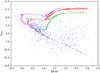 |
Fig. 4. Dereddened color-magnitude diagram for those sources with parallax measurements assuming AG = 2 and AG = 2 × E(BP − RP). Also shown are the isochrones for ages of 0.4 (magenta), 1 (red), and 10 (green) Gyr; see text for more details. |
4.6. Optical properties of the counterparts
As discussed in Sect. 4.1, we expect 98 X-ray sources with Gaia EDR3 listed counterparts. For further discussion we now introduce three groups of objects. Group 1 comprises those objects that have a Gaia EDR3 counterpart and a significant parallax measurement, group 2 those objects that have a Gaia EDR3 counterpart without a significant parallax measurement, and group 3 those objects that have no Gaia EDR3 listed counterpart. If Gaia EDR3 were complete, the group 3 objects would all have g magnitudes below the Gaia cutoff of about g ≈ 20.5; however, as discussed in Sect. 4.2, in the Chandra core region Gaia EDR3 is already incomplete at brighter magnitudes.
To assess the effects of incompleteness on the apparent magnitude distribution of the Gaia identified counterparts, we first consider the apparent magnitude distribution of the group 1 objects (blue curve) and group 2 objects (red curve) shown in Fig. 5. As is clear from Fig. 5, the large majority of the group 1 objects are brighter than 18 mag (only 2 out of 22 are fainter); on the other hand, most of the group 2 objects are fainter than 18 mag, and only 7 (out of 76) are brighter than 18 mag. This implies that group 1 objects remain essentially unaffected by incompleteness effects, while the opposite is true for group 2 objects. From Fig. 2 we can estimate the fraction of sources missed by Gaia as a function of magnitude, and thus correct the number of observed matches, assuming of course that the fraction of matches remains the same in the Gaia detected and missed sources; the derived corrected histograms are shown as dotted curves in Fig. 5. While the brighter sources with parallax remain essentially unaffected, the number of sources with Gaia matches without parallax can increase (by more than a factor of 2); however, the majority of these missed sources is expected to have magnitudes around g ≈ 20. The remaining ≈100 sources ought to remain below the actual Gaia cutoff and be fainter than 20.5 mag.
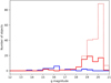 |
Fig. 5. Apparent magnitude distribution for Gaia matched sources with parallax (blue histogram) and Gaia matched sources without parallax (red histogram). The dotted histograms have been corrected for the effects of incompleteness; see text for more details. |
4.7. Spectral properties of the X-ray sources
In this section we focus on the spectral properties of the X-ray sources in the Chandra core region, using the formalism presented in Sect. 3.2.1. In Fig. 6 we present the q1 − q2-plane for the 318 X-ray sources in the core region; the blue data points denote Gaia sources with parallax (i.e., normal stars), the red data points denote Gaia sources without parallax but with magnitude and color information, and the green data points denote sources with counterparts below the faint Gaia limit.
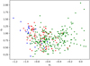 |
Fig. 6. q1 − q2 for X-ray sources in the core region. The blue data points denote Gaia sources with parallax, red data points denote Gaia sources without parallax, green data points denote sources with counterparts below the faint Gaia limit. |
It is clear that the differently colored data points populate different regions in the q1 − q2-plane shown in Fig. 6. The confirmed stars (blue data points) are located below q1 ≈ −0.7 and above q2 ≈ 0.9; the red data points partially overlap with the stars, but extend to larger q1-values (i.e., they have larger median energies); and the unidentified sources without Gaia counterparts also partially overlap with the blue and red data points, but extend to even higher medium energies. This finding is in line with expectations since stellar sources, first, are known to have softer spectra, and second, are located nearer to the Sun and should be statistically less affected by absorption effects.
4.8. Ratio of X-ray to optical fluxes
Next we consider the ratio of X-ray to optical fluxes for the sources in the Chandra core region. To convert the observed Chandra count rates into fluxes, we assume the sources to be coronal and use an ECF of 4.5 × 10⁻¹² erg cm−2 cnt−1, which refers to the absorbed flux in the 0.2−2.3 keV energy band; to convert from g magnitude to energy flux in the GaiaG band, we use Eq. (5). The resulting fX/fg values are shown in Fig. 7, both for objects with parallax (blue data points) and without parallax information (red data points). We note that no attempt has been made to correct the Chandra data points for absorption effects. To do this one would have to multiply the observed fX/fg ratios by the attenuation ratio provided in the last column of Table 1. For lower values of absorptions these corrections are close to unity, while for large values correction factors of more than an order of magnitude could result; we note that these corrections would push the fX/fg ratios plotted in Fig. 7 downward.
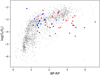 |
Fig. 7. Observed fX/fg ratios for X-ray sources with Gaia counterparts and parallax (blue data points) and with Gaia counterparts but no parallax (red data points). For comparison we also plot the fX/fg ratios derived by Schneider et al. (2022) for the coronal sources in the eROSITA EFEDS-field (small black data points); see text for more details. |
The fX/fg ratios observed in the Chandra deep field agree reasonably well with those derived by Schneider et al. (2022) in the eROSITA EFEDS-field; many of the identified Chandra X-ray sources have colors in excess of BP − RP = 3, and we expect these sources to be substantially affected by absorption. For the majority of the X-ray sources detected in the Chandra deep field we have no optical counterpart in Gaia EDR3 and hence no measured fX/fg ratio. Because of the completeness issues of Gaia in the Chandra deep field discussed in Sect. 4.3 the maximum brightness of any optical counterpart could be up to mag 18, but we expect the vast majority of counterparts to be fainter than mag 20.5, and therefore the expected fX/fg ratios would be far higher than is normally observed for coronal sources, clearly suggesting that these sources cannot be of coronal origin.
4.9. Distances and color-magnitude diagram of the Gaia matched sources
Only 22 of the 98 Gaia matched sources have significant parallax measurements, which allows us to compute distances and X-ray luminosities for these objects. The median distance of these 22 sources is 1.3 kpc, while the nearest source is located at a distance of 431 pc. It is of interest to investigate the CMD of these sources, which is displayed in Fig. 8 together with the isochrones as in Fig. 4; we note that here we assumed AG = 1.5 since these stars are not that distant from the Sun. Figure 8 shows that the majority of counterparts seem to be on or near the main sequence of spectral G and K. Some stars may be somewhat evolved; there is, however, only one object that appears to be on the horizontal branch. There are five very red objects with BP − RP colors in excess of 1.5; whether the red color is due to unaccounted-for reddening or intrinsic is unclear at the moment.
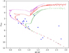 |
Fig. 8. Color-magnitude diagram of counterparts with parallax information. Also shown are the isochrones for ages of 0.4 (magenta), 1 (red), and 10 (green) Gyr; see text for more details. |
4.10. Iron line emission
Here we consider the appearance of iron line emission near 6.7 keV in the X-ray spectra of our sample stars. As is well known, there is no iron line at 6.7 keV; rather, there exists a whole series of iron lines arising from iron in ionization stages Fe XXI to Fe XXV in the spectral range between 6542 eV to 6698 eV (see, e.g., the line lists by Mewe et al. 1985). Doschek et al. (1981) present some examples of high-resolution spectra from solar flares, which show dozens of emission lines in the spectral range between 6.5 keV and 6.7 keV. As a consequence, in the lower resolution Chandra CCD spectra these lines remain unresolved, and the line centroid and width depend on the (unknown) temperature distribution in the line emitting regions. We therefore define the iron line band as the spectral region between 6.5 keV and 6.7 keV, a region which ought to contain the bulk of the expected emission and which is also matched to the energy resolution of the ACIS-I CCDs.
4.10.1. Spatial distribution
Focusing on the Chandra core region, we extract 3228 valid counting events with nominal energies in the range 6500 eV to 6700 eV, in the iron line band. As discussed by Revnivtsev et al. (2009), the majority of these counting events are caused by energetic particles, thus they are unrelated to astrophysical sources. Again following Revnivtsev et al. (2009), we use the ACIS stowed background (i.e., an observation with valid events but obtained with the ACIS-I camera not exposed to the sky) to estimate this particle background3. Using the energy band in the range 7.8−9.2 keV as a reference background band (and thus avoiding spectral regions with stronger fluorescent emission), we find a scaling of 0.107 for the counts recorded in our iron line band and this background reference band.
In our Chandra core region, which was exposed to the sky, the background reference band should be practically devoid of true X-ray photon events since the ACIS-I effective areas are very small indeed above an energy of 7 keV. Therefore, applying the same scaling, we expect 2875.9 events in the iron band to be caused by particle events, leaving the remaining 352.1 events to true X-ray photons. It is difficult to attach a serious error to this number; the statistical error alone would be about 2%, the true error might be 5−10%. It is clear, however, that the vast majority of events ought not to be associated with X-ray sources as already concluded by Revnivtsev et al. (2009), and we must develop a robust method to estimate the number of photons associated with the detected X-ray sources.
4.10.2. Nearest neighbor distribution
To isolate those counting events that can be associated with the detected X-ray sources (in the 0.5–7 keV energy band), we compute the NND between the detected 318 X-ray sources and the 3211 iron line range counting events. For each of the 3211 counting events we can determine the nearest X-ray source and compute the corresponding angular distance. The resulting distribution is shown in Fig. 9, together with two analytical fits following the nearest neighbor formula in Eq. (7). Clearly, the narrow distribution (shown in green in Fig. 9) is to be associated with true source photons, the rest is due to background, and integrating the green curve in Fig. 9 we estimate Nsource = 237(±20) source events; we expect 237 counting events to be associated with the 318 X-ray sources, thus a significant portion of these sources will not even contribute to the iron line range.
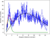 |
Fig. 9. Nearest neighbor distribution between detected X-ray sources and iron line range counting events (blue data points), together with analytical fits following Eq. (7) for source events (green curve), background events (black curve), and summed events (red curve); for more details see text. |
To specifically identify those events that are likely associated with the known X-ray sources, we can compute, from the model curves shown in Fig. 9, the probabilities of finding a true versus a spurious source photon as a function of the separation to the nearest source for all events registered in the iron line region. From these numbers we can compute the association completeness, which is the fraction of correctly attributed source events with respect to the true number, and the reliability, which is the fraction of correctly attributed events with respect to all events as a function of separation. The result of these computations is shown in Fig. 10, where we show the derived completeness and reliability fractions. Clearly we run into the conundrum that by choosing only highly reliable events, we miss many true events, while by increasing the completeness we also increase the contamination by including spurious events.
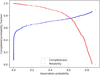 |
Fig. 10. Completeness (red data points) and reliability (blue data points) versus association probability; for more details see text. |
4.10.3. Iron line contamination and source identifications
Naturally, we expect contamination, as is obvious by considering the following numbers: given 3243 counting events in the Chandra core region and using a detection cell radius of 1.3 arcsec, we expect 0.17 counts per detection cell just by chance. Since this experiment is repeated 318 times, we expect ≈53 background counts that are located inside the detection cells and that we would identify with iron line events, although they are actually random. To address the contamination problem we compute, for every single counting event, the probability of being associated with one of the 318 detected X-ray sources just on the basis of geometry. From these probabilities we can then compute the probability with which any given source is associated with an event in the iron line region and display the resulting probability distribution histogram in Fig. 11. We find that 139 (out of 318) sources have very small association probabilities (and are not shown in Fig. 11), while 80 sources have association probabilities in excess of 0.8. The remaining 99 sources are in the gray zone, with some of them being likely to make some small contributions to the overall iron line emission.
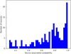 |
Fig. 11. Histogram representation of the association probability of the 318 detected X-ray sources with counting events in the iron line region; see text for more details. |
With the computed association probabilities we can proceed to recalculate the q1 − q2 diagrams, but separated by source association probability and the groups defined for Fig. 6. The essential contribution to the iron line complex comes from the sources with association probabilities passoc > 0.8, which contains only two stars and nine objects listed in Gaia EDR3, and is clearly dominated by the (green) sources that cannot be associated with Gaia entries. Moving to sources with lower association probabilities, the number of stars increases and the sources tend to become softer, a clear indication that they contribute little or nothing to the emission in the iron line region. Inspecting the detailed count statistics, we find that only 25 sources, less than 10% of the total, are responsible for more than 50% of the overall observed signal (see Fig. 12).
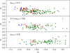 |
Fig. 12. q1 − q2 for X-ray sources in the core region with color-coding as in Fig. 6 and separated into sources with association probability < 30% (upper panel), in the range 30%−80% (middle panel), and > 80% (lower panel); see text for more details. |
4.10.4. Iron line intensity
Having identified those X-ray sources that actually significantly contribute to the iron line emission, we can construct a stacked spectrum of all high-probability sources contributing to the relevant spectral region around 6.7 keV (i.e., those with p > 0.8). This stacked (raw) X-ray spectrum is shown in Fig. 13 (blue data points), together with two model fits. The first model (Model 1, in red) assumes a linear curve with a single Gaussian line superimposed; this means that the model has five parameters, two for the continuum and three for the line. The second model (Model 2, in magenta) assumes an additional second line at a fixed line energy of 6.965 keV, with the width of the two lines being equal. The latter model then has an additional sixth free parameter, and the obtained fit parameters (for the lines) are summarized in Table 2, with the central energy and amplitude (as well as the background) being free fit parameters.
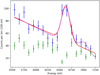 |
Fig. 13. Stacked X-ray spectrum of all X-rays sources contributing to the iron line complex with a probability of at least 80%. |
As is seen in Fig. 13 and Table 2, the chosen descriptions clearly provide adequate fits to the Chandra data. The improvement in fit quality by introducing a second line is marginal, and from a formal point of view this introduction is not completely justified; while the reduced value of the χ2 test statistics,  , is a little lower, the Akaike Information Criterion (AIC) values of the two solutions are very similar. The central energy of the higher energy line was intentionally set to the energy of the Lyα line of Fe XXVI, while we interpret the lower energy, stronger line as a mixture of Fe lines in ionization stages XXIII–XXV; the central wavelength agrees well with the centroid of a variety of iron lines appearing in solar flares (cf. the flare spectra presented by Doschek et al. 1981). An astrophysical discussion of these results is given in Sect. 5.
With our simple model we estimate a total line count of ≈130 counts in this lower energy iron line complex (i.e., 40% of the total signal in the iron line region is continuum); the higher energy line, if considered real, would contribute another 30% of line signal. Also shown in Fig. 13 (green data points) is a stacked X-ray spectrum of the remaining sources with low association probability (i.e., p < 0.8). Clearly, these sources provide no measurable contribution to the iron line region, and at energies above 7 keV the observed signal is consistent with particle background according to expectations.
Converting the measured counts contained in the iron line complex (rather than the continuum) corresponds to an intensity of 4.1 × 10⁻⁹ erg s−1 cm−2 ster−1 at the position of the Chandra deep field. Assuming that the emission in the iron line complex is produced by a plasma in thermal equilibrium, it is important to realize that only a very hot plasma can produce significant flux in this complex. To illustrate this temperature sensitivity it is useful to consider (for the sake of simplicity for an isothermal plasma) the X-ray flux ratio in the iron line complex (i.e., between 6.5 and 6.7 keV and above the continuum) and the ROSAT band in the range 0.2−2.4 keV, in which measurements of tens of thousands of stars are available. These calculations were carried out with the most recent CHIANTI package (Del Zanna et al. 2021). As demonstrated in Fig. 14, where we plot this flux ratio as a function of temperature, the flux in the iron line complex can reach a small percentage of the measured flux in the lower energy band, but only for temperatures distinctly above 107 K. An inspection of the Fe ionization equilibrium immediately shows that only at those temperatures are the necessary Fe ionization stages produced. For temperatures below 107 K, any flux in the iron line complex is essentially unmeasurable.
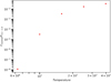 |
Fig. 14. Expected ratio of X-ray flux in the iron line complex to flux in the energy band 0.2 keV−2.4 keV for a plasma in collisional equilibrium. |
5. Discussion
5.1. Iron line intensity
We specifically studied the iron line region in the range 6.5−6.7 keV and confirm that up to 90% of the signal recorded in the Chandra data in that spectral region are caused by particle events. As a consequence, there is a contamination problem, in the sense that the observed counting events with energies between 6.5 and 6.7 keV need not necessarily be associated with any X-ray source but rather with particle background. We developed a statistical method to associate the observed counts in the actual iron line region with the detected X-ray sources; our analysis further shows that ≈140 counts are contained in the iron line complex (rather than the continuum). With this number we can compute an iron line intensity of 4.1 × 10⁻⁹ erg s−1 cm−2 ster−1 at the position near the Chandra deep field. Ignoring absorption effects (which ought to be very small at 6.7 keV) and assuming a population of sources with uniform space density nO with a mean luminosity in the iron line complex of  , distributed over a distance R, we compute an iron line intensity IFe of
thus our intensity measurement does constrain the product between source density and luminosity in the iron line, which we determine, using R = 8 kpc, as

Our choice of R = 8 kpc is a compromise. If the relevant GRXE source population is confined to the bulge of the Milky Way, a choice of R = 4 kpc might be more appropriate; however, if the source population extends to the other side of the Galaxy, we should choose R = 16 kpc. Thus, a systematic error of a factor of around two is present in our estimate of R and hence nO.
5.2. Possible contribution of M dwarfs
We next discuss possible coronal source classes that might be held responsible for the observed GRXE. The most abundant class of normal nondegenerate stars are M dwarfs, which are characterized by (unreddened) colors of BP − RP > 2. Unfortunately, only 51 out the 98 X-ray sources identified with Gaia EDR3 entries have color information, and only 28 of those have BP − RP colors in excess of 2. Assuming then a typical reddening of AG ≈ 2 (see discussion in Sect. 3.1), M dwarfs would be expected to have BP − RP colors in excess of 3, which applies to only 11 of these objects. As far as the objects with parallax information are concerned (see Fig. 8), at most two (out of 22) objects can be argued to be M dwarfs.
Assuming that the Gaia census is complete down to a limiting magnitude of 18.5 and a mean absorption of AG ∼ 2, we compute a limiting distance of about 450 pc, at which an M0 dwarf with an absolute G magnitude of 8.2 would appear at the magnitude limit; if detected at the X-ray flux limit of 5 × 10⁻¹⁶ erg cm−2 s−1, an X-ray luminosity of about 1 × 1028 erg s−1 would result. Among the detected X-ray sources with parallax, there are at most two that could qualify as M dwarfs and are located within the limiting distance. Converting this to a space density of M dwarfs with X-ray luminosities of at least 2 × 1028 erg s−1, one computes an estimate of at most ≈0.02 pc−3. From Eq. (10) such a space density would require a mean  luminosity of 3 × 1027 erg s−1, which in turn would correspond to a typical X-ray luminosity (in the ROSAT band) of a few times 1029 erg s−1, far larger than observed.
Finally, we consider the spectral properties of M dwarfs. Unfortunately, systematic studies of the strength of the iron line in various stellar samples have not been carried out; only the ongoing eROSITA survey will eventually yield the necessary numbers in unbiased all-sky samples. For the time being we have to use extrapolations like those shown in Fig. 14. According to Schmitt et al. (1995) the mean X-ray luminosity of M dwarfs in the solar neighborhood is the range 3 − 8 × 1027 erg s−1, depending on which samples are being considered. If all M dwarfs had coronal temperatures in excess of 107 K, we would still require space densities far higher than observed; however, iron line emission is observed in M dwarfs typically only in large flares near flare peak. A nice and detailed example of such an event on the nearby M dwarf CN Leo is presented by Liefke et al. (2010). Based on these lines of evidence, we conclude that (coronally emitting) M dwarfs and related systems are an extremely unlikely source of the observed GRXE emission since their space densities and X-ray temperatures are too low.
5.3. Possible contribution of active binary systems
Let us now turn to RS CVn and similar binary systems, which are the most luminous known coronal X-ray sources. Unfortunately, truly volume-limited and complete samples of these objects are not available. A comprehensive ROSAT X-ray survey comprising 136 optically pre-selected such systems has been presented by Dempsey et al. (1993), who find RASS detections in 112 systems, yielding a detection rate of more than 80%. The typical X-ray luminosities of these systems are found to be in the range 1029 erg s−1–1032 erg s−1, and similar numbers apply to Algol systems, which also contain rapidly rotating evolved late-type stars. Considering the RS CVn sample studied by Dempsey et al. (1993) and concentrating on systems located within 100 pc and with X-ray luminosities in excess of 1030 erg s−1, we find 38 systems (out of 50); instead, when requiring X-ray luminosities in excess of 1031 erg s−1, we end up with 8 (out of 50) systems. Assuming now the sample of Dempsey et al. (1993) to be more or less complete within 100 pc, these numbers translate into space densities of ≈9 × 10⁻⁶ pc−3 for systems with LX > 1030 erg s−1, and ≈2 × 10⁻⁶ pc−3 for systems with LX > 1031 erg s−1 (in the ROSAT band 0.2−2.4 keV). Returning now to the Chandra deep field, we can detect, with a flux limit of 5 × 10⁻¹⁶ erg s−1 cm−2, objects with LX > 1030 erg s−1 out to about 4 kpc, and objects with LX > 1031 erg s−1 out to about 13 kpc. Inspecting the calculated X-ray luminosities for those objects for which parallax and colors are available, we actually find that all objects have X-ray luminosities below 1030 erg s−1; based on this finding we estimate an upper limit to the space density of active binary systems with LX > 1030 erg s−1 as < 2 × 10⁻⁵ pc−3, which is actually consistent with the estimates derived form the local survey of Dempsey et al. (1993).
As far as 6.7 keV iron line emission is concerned, we are not aware of systematic and complete surveys for the 6.7 keV iron line in these systems; however, as is true for M dwarfs, the line is known to appear in flares, a nice example of which is presented (for the case of Algol) by Favata & Schmitt (1999) and for the case of the active binary system II Peg by Osten et al. (2007). Assuming now that the space density of these system is 10−5 pc−3, we require from Eq. (10) a 6.7 keV (mean) luminosity of about 5 × 1030 erg s−1, which would translate into broadband X-ray luminosities of about 5 × 1032 erg s−1, assuming a (rather) optimistic iron line fraction of 1% (Fig. 14). However, such mean X-ray luminosities are simply not observed. An in-depth analysis of the eROSITA data will eventually yield far more accurate numbers both for the space density and iron line properties of these systems; however, given our current knowledge active binary systems are not likely to contribute significantly to the GRXE.
5.4. Possible contribution of cataclysmic variables
We now turn to cataclysmic variables (CV) as possible sources of the GRXE. It is very difficult to construct complete samples of CVs; for example, Pretorius & Knigge (2012) present a complete X-ray selected sample of nonmagnetic CVs in the region of the north ecliptic pole and the ROSAT bright survey, and derive a space density of 4 × 10⁻⁶ pc−3 for such systems, but these authors note at the same time that their two surveys are likely have failed to detect a large, faint population of short-period CVs, and that hence the true space density may well be a factor of 2 or 3 larger. Thus, it appears to be fair to conclude that the space density of such systems is highly uncertain at best.
Xu et al. (2016) present a detailed study of Fe line diagnostics in a sample including symbiotic stars (SS, 6 studied objects), polars (P, 3), intermediate polars (IP, 16), dwarf novae in quiescence (DN, 16), and active binaries (AB, 4), based on Suzaku observations of these sources. In particular, Xu et al. (2016) measure the equivalent widths of the 6.4 keV fluorescent line arising from neutral or weakly ionized material, and the 6.7 keV and 7.0 iron lines arising from highly ionized material. As already pointed out, strictly speaking there are no 6.7 keV and 7.0 keV iron lines, as is evidenced, for example, by inspecting the line lists by Mewe et al. (1985); the 7.0 keV line is produced by hydrogen- and helium-like iron, while the 6.7 keV line is predominantly produced by somewhat lower ionization stages, leading to the temperature diagnostics employed by Xu et al. (2016).
Clearly, the samples used by Xu et al. (2016) can hardly be considered complete; even so, the spectral studies performed by (cf. Table 3 in Xu et al. 2016) reveal some interesting results. For the SS and IP sources the 6.4 keV and 6.7 keV lines have about equal equivalent widths, while for the P and DN sources the 6.4 keV line is much weaker or absent (cf. Table 2 in Xu et al. 2016) and it is entirely absent in the four AB sources studied by Xu et al. (2016). The latter finding is in line with what we know from stellar coronae, where one finds the 6.4 keV fluorescent line only in rather exceptional cases (cf. the discussion presented by Czesla & Schmitt 2010). In the Fe spectrum of the stacked sources in the Chandra deep field (Fig. 13), only the 6.7 keV line is clearly visible; there are hints of a feature at 7.0 keV (Sect. 4.10.4), yet the 6.4 keV fluorescent feature remains clearly undetected. As a consequence we conclude that (to the extent that the samples presented by Xu et al. 2016 are indeed representative) SS and IP sources cannot contribute significantly to the GRXE (at least in the Chandra deep field). Our work excludes coronal sources, thus we are left with DN and P sources as possible contributors to the GRXE. We also note that the ratio of the 7.0 keV to the 6.7 keV line measured in the stacked spectrum is consistent with the numbers reported by Xu et al. (2016) for the DN and P sources.
Assuming a space density of 4 × 10⁻⁶ pc−3 as derived by Pretorius & Knigge (2012) as appropriate space density, we require a mean iron line luminosity  erg s−1, which is about the same as the broadband luminosity (in the 2−10 keV band) reported by Xu et al. (2016) and the X-ray luminosities reported by Pretorius & Knigge (2012) in the ROSAT band. Considering the ratio of the iron line flux in the 6.7 keV feature (from Table 3 in Xu et al. 2016) and the broadband flux (in the 2−10 keV band from Table 2 in Xu et al. 2016), we find values typically between 0.1 and 0.01, and lower values would result if one were to use the ROSAT band as reference. As a consequence, if these CVs are indeed the sources of the GRXE, their space densities would have to be higher than 4 × 10⁻⁶ pc−3, the space density derived by Pretorius & Knigge (2012).
6. Conclusions
The conclusions of our study of the Chandra deep field observations can be concisely summarized as follows:
-
A meaningful identification of the detected X-ray sources with entries in the Gaia EDR3 catalog can be carried out thanks to the excellent Chandra source positions, with a contamination below 10%.
-
Only a relatively small fraction (about 30%) of the X-ray sources can be identified with Gaia EDR3 entries, and only about 7% can be meaningfully placed into a color-magnitude diagram. Due do the high source density in the Chandra deep field, Gaia EDR3 is complete only to about 18.5 mag; individual absorption measurements of the counterparts are highly desirable.
-
The CMD (Fig. 4) of the Gaia identified X-ray counterparts with both parallax and color information shows that the majority of these objects are of spectral types F and G; many of these systems may actually be located above the main sequence, consistent with interpreting these systems as RS CVn and related systems.
-
Only a small fraction of the detected X-ray sources contribute to the observed 6.7 keV iron line emission. The pure iron line intensity (i.e., continuum subtracted) in the Chandra deep field is 4 × 10⁻¹² erg s−1 cm−2 deg−2.
-
In addition to the clearly detected 6.7 keV iron line, there are hints of another Fe line at 7.0 keV; while strictly statistically not significant, this line could be interpreted as FeXXVI Lyα. The fluorescent 6.4 keV line is not detected in the Chandra deep field.
-
We demonstrate that coronal sources (specifically M dwarfs), the most abundant class of stars, and RS CVn systems, the most X-ray luminous class of stars, provide only small contributions to the observed X-ray source census and insignificant contributions to the observed iron line intensity.
We therefore expect that more X-ray luminous objects with lower space density provide the bulk of the observed GXRE emission, possibly the somewhat peculiar class of magnetic cataclysmic variables identified by Hong et al. (2012) in the Chandra deep field. If the results of the Fe line characteristics derived by Xu et al. (2016) can be extended to the CV population at large, dwarf novae and polars would then be the main contributors to the GRXE. Thus, in summary, an accurate attribution of the X-ray emission observed in the Chandra deep field to individual source classes remains challenging. To alleviate the whole situation, a reliable determination of the space densities of the various CV populations is urgently called for.
Derived from the material available on the website http://svo2.cab.inta-csic.es/theory/fps/index.php?mode=browsegname=GAIAgna
For more information on the ACIS-I stowed background we refer to the website https://cxc.cfa.harvard.edu/contrib/maxim/stowed/
Acknowledgments
This research has made use of data obtained from the Chandra Data Archive and the Chandra Source Catalog, as well as software provided by the Chandra X-ray Center (CXC). This research has further made use of data from the European Space Agency (ESA) mission Gaia (https://www.cosmos.esa.int/gaia), processed by the Gaia Data Processing and Analysis Consortium (DPAC, https://www.cosmos.esa.int/web/gaia/dpac/consortium). Funding for the DPAC has been provided by national institutions, in particular the institutions participating in the Gaia Multilateral Agreement. This research has also made use of the SIMBAD database, operated at CDS, Strasbourg, France. X-ray astronomy at Hamburg Observatory is supported by the DFG funded research group eRO-STEP (FOR 2990). Finally we thank an anonymous referee for help in improving this paper and removing errors.
References
- Andrae, R., Fouesneau, M., Creevey, O., et al. 2018, A&A, 616, A8 [NASA ADS] [CrossRef] [EDP Sciences] [Google Scholar]
- Bressan, A., Marigo, P., Girardi, L., et al. 2012, MNRAS, 427, 127 [NASA ADS] [CrossRef] [Google Scholar]
- Czesla, S., & Schmitt, J. H. M. M. 2010, A&A, 520, A38 [NASA ADS] [CrossRef] [EDP Sciences] [Google Scholar]
- Del Zanna, G., Dere, K. P., Young, P. R., & Landi, E. 2021, ApJ, 909, 38 [NASA ADS] [CrossRef] [Google Scholar]
- Dempsey, R. C., Linsky, J. L., Fleming, T. A., & Schmitt, J. H. M. M. 1993, ApJS, 86, 599 [NASA ADS] [CrossRef] [Google Scholar]
- Doschek, G. A., Feldman, U., & Cowan, R. D. 1981, ApJ, 245, 315 [NASA ADS] [CrossRef] [Google Scholar]
- Ebisawa, K., Maeda, Y., Kaneda, H., & Yamauchi, S. 2001, Science, 293, 1633 [NASA ADS] [CrossRef] [Google Scholar]
- Evans, I. N., Primini, F. A., Glotfelty, K. J., et al. 2010, ApJS, 189, 37 [NASA ADS] [CrossRef] [Google Scholar]
- Fabricius, C., Luri, X., Arenou, F., et al. 2021, A&A, 649, A5 [NASA ADS] [CrossRef] [EDP Sciences] [Google Scholar]
- Favata, F., & Schmitt, J. H. M. M. 1999, A&A, 350, 900 [NASA ADS] [Google Scholar]
- Fleming, T. A., Giampapa, M. S., Schmitt, J. H. M. M., & Bookbinder, J. A. 1993, ApJ, 410, 387 [NASA ADS] [CrossRef] [Google Scholar]
- Gaia Collaboration (Prusti, T., et al.) 2016, A&A, 595, A1 [NASA ADS] [CrossRef] [EDP Sciences] [Google Scholar]
- Garmire, G. P., Bautz, M. W., Ford, P. G., Nousek, J. A., & Ricker, G. R., Jr. 2003, in X-ray and Gamma-ray Telescopes and Instruments for Astronomy, eds. J. E. Truemper, & H. D. Tananbaum, SPIE Conf. Ser., 4851, 28 [NASA ADS] [CrossRef] [Google Scholar]
- Güdel, M. 2004, A&ARv, 12, 71 [CrossRef] [Google Scholar]
- Hong, J. 2012, MNRAS, 427, 1633 [NASA ADS] [CrossRef] [Google Scholar]
- Hong, J., van den Berg, M., Grindlay, J. E., Servillat, M., & Zhao, P. 2012, ApJ, 746, 165 [NASA ADS] [CrossRef] [Google Scholar]
- Liefke, C., Fuhrmeister, B., & Schmitt, J. H. M. M. 2010, A&A, 514, A94 [NASA ADS] [CrossRef] [EDP Sciences] [Google Scholar]
- Mewe, R., Gronenschild, E. H. B. M., & van den Oord, G. H. J. 1985, A&AS, 62, 197 [NASA ADS] [Google Scholar]
- Molaro, M., Khatri, R., & Sunyaev, R. A. 2014, A&A, 564, A107 [NASA ADS] [CrossRef] [EDP Sciences] [Google Scholar]
- Morihana, K., Tsujimoto, M., Yoshida, T., & Ebisawa, K. 2013, ApJ, 766, 14 [NASA ADS] [CrossRef] [Google Scholar]
- Osten, R. A., Drake, S., Tueller, J., et al. 2007, ApJ, 654, 1052 [NASA ADS] [CrossRef] [Google Scholar]
- Pecaut, M. J., & Mamajek, E. E. 2013, ApJS, 208, 9 [Google Scholar]
- Predehl, P., & Schmitt, J. H. M. M. 1995, A&A, 500, 459 [Google Scholar]
- Pretorius, M. L., & Knigge, C. 2012, MNRAS, 419, 1442 [NASA ADS] [CrossRef] [Google Scholar]
- Revnivtsev, M., Molkov, S., & Sazonov, S. 2006, MNRAS, 373, L11 [NASA ADS] [CrossRef] [Google Scholar]
- Revnivtsev, M., Sazonov, S., Churazov, E., et al. 2009, Nature, 458, 1142 [Google Scholar]
- Schmitt, J. H. M. M., Fleming, T. A., & Giampapa, M. S. 1995, ApJ, 450, 392 [Google Scholar]
- Schmitt, J. H. M. M., Czesla, S., Freund, S., Robrade, J., & Schneider, P. C. 2022, A&A, in press, https://doi.org/10.1051/0004-6361/202141132 [Google Scholar]
- Schneider, P. C., Freund, S., Czesla, S., et al. 2022, A&A, in press, https://doi.org/10.1051/0004-6361/202141133 [Google Scholar]
- Worrall, D. M., & Marshall, F. E. 1983, ApJ, 267, 691 [NASA ADS] [CrossRef] [Google Scholar]
- Worrall, D. M., Marshall, F. E., Boldt, E. A., & Swank, J. H. 1982, ApJ, 255, 111 [Google Scholar]
- Xu, X.-J., Wang, Q. D., & Li, X.-D. 2016, ApJ, 818, 136 [NASA ADS] [CrossRef] [Google Scholar]
Appendix A: Chandra and Gaia source identifications
Here we present the table with our successful Gaia identifications.
List of Gaia matched X-ray sources in Chandra core region. Columns (1) and (2) provide the respective Chandra and Gaia EDR3 identifications; column (3) provides the geometric association probability; columns (4) to (7) contain the g magnitude, BP-RP color, parallax, and parallax over error as provided in Gaia EDR3. The flag “Star” denotes a coronal source.
All Tables
Energy conversion factors (absorbed and unabsorbed), X-ray and G band absorptions, and attentuation ratios in the optical and X-ray band for various values of interstellar absorption column densities.
List of Gaia matched X-ray sources in Chandra core region. Columns (1) and (2) provide the respective Chandra and Gaia EDR3 identifications; column (3) provides the geometric association probability; columns (4) to (7) contain the g magnitude, BP-RP color, parallax, and parallax over error as provided in Gaia EDR3. The flag “Star” denotes a coronal source.
All Figures
|
Fig. 1. Nearest neighbor distribution between the X-ray sources in the Chandra core region and the Gaia entries. The yellow curve denotes a fit of a Rayleigh distribution to the true matches, the nearest neighbor distribution to the random matches is shown in green, and the summed curve in red; see text for details. |
| In the text | |
|
Fig. 2. Number of objects vs. g-magnitude for all Gaia entries in the Chandra core region (blue data points); the red data points show a hypothetical Chandra core region log N–log S curve without any incompleteness effects; see text for more details. |
| In the text | |
|
Fig. 3. Observed color-magnitude diagram for Gaia entries in the Chandra core region. The blue data points have parallax measurements with S/N > 3, the red data points do not. The black arrow indicates the reddening vector; the region in the upper left is where Gaia EDR3 is complete and where proper stars ought to be located; see text for more details. |
| In the text | |
|
Fig. 4. Dereddened color-magnitude diagram for those sources with parallax measurements assuming AG = 2 and AG = 2 × E(BP − RP). Also shown are the isochrones for ages of 0.4 (magenta), 1 (red), and 10 (green) Gyr; see text for more details. |
| In the text | |
|
Fig. 5. Apparent magnitude distribution for Gaia matched sources with parallax (blue histogram) and Gaia matched sources without parallax (red histogram). The dotted histograms have been corrected for the effects of incompleteness; see text for more details. |
| In the text | |
|
Fig. 6. q1 − q2 for X-ray sources in the core region. The blue data points denote Gaia sources with parallax, red data points denote Gaia sources without parallax, green data points denote sources with counterparts below the faint Gaia limit. |
| In the text | |
|
Fig. 7. Observed fX/fg ratios for X-ray sources with Gaia counterparts and parallax (blue data points) and with Gaia counterparts but no parallax (red data points). For comparison we also plot the fX/fg ratios derived by Schneider et al. (2022) for the coronal sources in the eROSITA EFEDS-field (small black data points); see text for more details. |
| In the text | |
|
Fig. 8. Color-magnitude diagram of counterparts with parallax information. Also shown are the isochrones for ages of 0.4 (magenta), 1 (red), and 10 (green) Gyr; see text for more details. |
| In the text | |
|
Fig. 9. Nearest neighbor distribution between detected X-ray sources and iron line range counting events (blue data points), together with analytical fits following Eq. (7) for source events (green curve), background events (black curve), and summed events (red curve); for more details see text. |
| In the text | |
|
Fig. 10. Completeness (red data points) and reliability (blue data points) versus association probability; for more details see text. |
| In the text | |
|
Fig. 11. Histogram representation of the association probability of the 318 detected X-ray sources with counting events in the iron line region; see text for more details. |
| In the text | |
|
Fig. 12. q1 − q2 for X-ray sources in the core region with color-coding as in Fig. 6 and separated into sources with association probability < 30% (upper panel), in the range 30%−80% (middle panel), and > 80% (lower panel); see text for more details. |
| In the text | |
|
Fig. 13. Stacked X-ray spectrum of all X-rays sources contributing to the iron line complex with a probability of at least 80%. |
| In the text | |
|
Fig. 14. Expected ratio of X-ray flux in the iron line complex to flux in the energy band 0.2 keV−2.4 keV for a plasma in collisional equilibrium. |
| In the text | |
Current usage metrics show cumulative count of Article Views (full-text article views including HTML views, PDF and ePub downloads, according to the available data) and Abstracts Views on Vision4Press platform.
Data correspond to usage on the plateform after 2015. The current usage metrics is available 48-96 hours after online publication and is updated daily on week days.
Initial download of the metrics may take a while.