| Issue |
A&A
Volume 661, May 2022
|
|
|---|---|---|
| Article Number | A56 | |
| Number of page(s) | 8 | |
| Section | The Sun and the Heliosphere | |
| DOI | https://doi.org/10.1051/0004-6361/202142497 | |
| Published online | 02 May 2022 | |
Simulations of solar radio zebras
Astronomical Institute of the Czech Academy of Sciences, Fričova 298, 251 65 Ondřejov, Czech Republic
e-mail: This email address is being protected from spambots. You need JavaScript enabled to view it.
Received:
21
October
2021
Accepted:
26
February
2022
Abstract
Context. Solar radio zebras are used in diagnostics of solar flare plasmas and it is of great importance to construct accurate models to correctly characterize them.
Aims. We simulated two zebras to verify their double-plasma resonance (DPR) model.
Methods. In our zebra simulations, we used the DPR model in an expanding and compressing part of the loop as well as with the wave propagating along the loop.
Results. Using the DPR model in such a loop, we successfully simulated zebras from the 1 August 2010 and 21 June 2011 flares. We found that increasing the density or decreasing the magnetic field in the part of the loop, where zebra-stripe sources are located, the zebra stripes are shifted to higher frequencies and vice versa. In the case of the 21 June 2011 flare, we confirm that small deviations of zebra-stripe frequencies from their mean values can be explained by waves propagating along the loop. We also confirm high values for the gyro-harmonic number of zebra stripes. We explain an inconsistency in the wave velocities derived from the plasma parameters and from the frequency drift in combination with the density model of the solar atmosphere. Finally, we discuss the high values of the gyro-harmonic number found in the studied zebras.
Key words: Sun: flares / Sun: radio radiation / Sun: oscillations
© ESO 2022
1. Introduction
Zebras or zebra patterns belong to the most remarkable fine structures of solar radio bursts. They are used in diagnostics of solar flare plasmas. In dynamic radio spectra, they appear in the form of regular emission stripes, which have been described in numerous papers and monographs (Kuijpers 1975; Slottje 1981; Chernov 2006, 2011; Tan et al. 2012, 2014). The most frequently used model to explain them is one based on the double plasma resonance (DPR) condition (Kuijpers 1975, 1980; Zheleznyakov & Zlotnik 1975; Mollwo 1983, 1988; Winglee & Dulk 1986; Zlotnik 2013)
 (1)
(1)
where fu, fp[MHz] = 9 × 10![Mathematical equation: $ ^{-3}\sqrt{n [\rm{cm}^{-3}]} $](/articles/aa/full_html/2022/05/aa42497-21/aa42497-21-eq2.gif) , and fc[MHz] = 2.8 B[G] are the upper-hybrid, electron-plasma, and electron-cyclotron frequencies, respectively, and n is the plasma density, B is the magnetic field, and s is the gyro-harmonic number that is constant for any continuous zebra stripe. In this model, it is also assumed that the upper-hybrid waves are converted to the observed electromagnetic waves via their merging with low-frequency waves or scattering on plasma particles. Thus, the frequency of the electromagnetic waves is nearly the same as for the upper-hybrid waves. This model is supported by positional observations carried out by the Owens Valley Solar Array (OVSA; Chen et al. 2011).
, and fc[MHz] = 2.8 B[G] are the upper-hybrid, electron-plasma, and electron-cyclotron frequencies, respectively, and n is the plasma density, B is the magnetic field, and s is the gyro-harmonic number that is constant for any continuous zebra stripe. In this model, it is also assumed that the upper-hybrid waves are converted to the observed electromagnetic waves via their merging with low-frequency waves or scattering on plasma particles. Thus, the frequency of the electromagnetic waves is nearly the same as for the upper-hybrid waves. This model is supported by positional observations carried out by the Owens Valley Solar Array (OVSA; Chen et al. 2011).
Diagnostics based on the DPR model of zebras enable the determination not only of the plasma density in the zebra-stripe sources (![Mathematical equation: $ {n}[{\rm cm}^{-3}]\,=\, f_s^2(1-1/s^2)/8.1 \times 10^{-5} $](/articles/aa/full_html/2022/05/aa42497-21/aa42497-21-eq3.gif) , where fs [MHz] is the zebra-stripe frequency taken to equal fu), but also the magnetic field strength, (B[G] = fs/(2.8s)). However, for this purpose, it is of upmost importance to determine the gyro-harmonic numbers corresponding to specific zebra stripes. Several methods for their determination have been developed. For example, there is a method based on comparisons of the zebra-stripe frequencies in the atmosphere with the exponential dependencies of plasma density and magnetic field (Karlický & Yasnov 2015). A graphical version of this method was used in estimating the density and magnetic field turbulence in the zebra source (Karlický & Yasnov 2020). While both these methods assumed the parameter R = Lb/Ln as constant, where Lb and Ln are the magnetic field and density scales along the vertically oriented loop, the more advanced method assumes the parameter R as a linear function of the gyro-harmonic number (Yasnov & Karlický 2020).
, where fs [MHz] is the zebra-stripe frequency taken to equal fu), but also the magnetic field strength, (B[G] = fs/(2.8s)). However, for this purpose, it is of upmost importance to determine the gyro-harmonic numbers corresponding to specific zebra stripes. Several methods for their determination have been developed. For example, there is a method based on comparisons of the zebra-stripe frequencies in the atmosphere with the exponential dependencies of plasma density and magnetic field (Karlický & Yasnov 2015). A graphical version of this method was used in estimating the density and magnetic field turbulence in the zebra source (Karlický & Yasnov 2020). While both these methods assumed the parameter R = Lb/Ln as constant, where Lb and Ln are the magnetic field and density scales along the vertically oriented loop, the more advanced method assumes the parameter R as a linear function of the gyro-harmonic number (Yasnov & Karlický 2020).
In recent zebra studies, changes in zebra-stripe frequencies around their mean values have been interpreted by a presence of turbulence or waves in the zebra source (Karlický & Yasnov 2020, 2021). This interpretation agrees with the result presented in the paper by Kaneda et al. (2018), where the authors found the propagating magnetosonic wave in the 21 June 2011 zebra event. Yasnov (2021) confirmed this wave and he determined the gyro-harmonic number for the zebra stripe with the lowest frequency greater than 129. (For more details, see Table 1 in Yasnov 2021.)
In the present paper, via simulations of observed zebras, we want to verify the DPR model of zebras. These simulations are according to our knowledge quite new. They differ from our previous studies. While in previous papers we determined plasma and wave parameters at selected time instants, here we are simulating the properties of observed zebras during their evolution. For the present study, we selected one zebra from the decimetric range and second one from the metric range. We also checked high values of the gyro-harmonic numbers, s, that were found in the analysis of several zebra events (Karlický & Yasnov 2021; Yasnov 2021). In particular, numerical simulations of the DPR instability show that the maximal growth rate of the upper-hybrid waves decreases when increasing the gyro-harmonic number, s (Benáček et al. 2017), and thus smaller values of s should be preferred. However, these simulations were made only for small values of s (<20) and in a limited space of plasma parameters. This problem will be discussed in the final section of this paper.
2. Simulation model
In the present model, we assume that zebras are generated by the double plasma resonance mechanism, namely, zebra-stripe sources are located at the regions where the DPR condition (relation (1)) is fulfilled and zebra-stripe frequencies correspond to the upper-hybrid frequencies at these regions. As mentioned in the introduction and shown in Fig. 1, zebra-stripe frequencies change in all zebra stripes similarly and simultaneously. These changes look to be synchronized. Moreover, if we look differences between the neighboring zebra-stripe frequencies in details, then their small variations in time can be seen. Just these small variations were studied in selected times during zebra evolution by Karlický & Yasnov (2021) and the waves propagating through zebra-stripe sources were found.
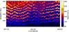 |
Fig. 1. Dynamic radio spectrum with the zebra observed on 1 August 2010 by the Ondřejov radiospectrograph (Jiřička & Karlický 2008). The arrow shows the zebra stripe chosen for the zebra-stripe fitting. |
Considering all the above-mentioned observational aspects of zebras, we propose the simulation model that consists of two processes: a) The process of compression and expansion of the part of the loop where zebra-stripe sources are located (Process A), which explains simultaneous and synchronized changes of all zebra-stripe frequencies; and b) the wave propagating through zebra-stripe sources (Process B), which explains quasi-periodic frequency changes of the frequency distance between neighboring zebra stripes. The schema of the simulation model in shown in Fig. 2.
 |
Fig. 2. Schema of the model. |
The synchronized variations of frequencies of all zebra stripes are usually much greater than the quasi-periodic variations of the frequency distance between neighboring zebra stripes. Thus, the changes of the plasma density and magnetic field in Process A are usually much greater than those in Process B.
In the model, we assume a vertically oriented part of the loop where zebra-stripe sources are located. The plasma density n in this part of the loop is described by the Aschwanden density model (Aschwanden 2002):
 (2)
(2)
where n1 = nQexp(−p), nQ = 4.6 × 108 cm−3, p = 2.38, and h is the height, h1 = 1.6 × 1010 cm. The magnetic field is expressed by the exponential function:
 (3)
(3)
In the present model, this relation is valid only at the heights of the zebra-stripe sources. In both the density and magnetic field models, h is the height above the photosphere. Thus, the magnetic field B0 (for h = 0) is useful only in calculations of the magnetic field at heights of zebra-stripe sources (however, we note that real values of the magnetic field at the photosphere can be quite different). In addition, Lb is the scale-height. The Aschwanden’s model is selected because it also covers plasma frequencies above 1000 MHz and it is based on radio observations.
In the model loop (Fig. 2), we indicated levels where the double-plasma resonance condition (relation (1)) is fulfilled and zebra-stripe sources are located. As mentioned above, for synchronization of the variations of zebra-stripe frequencies of all zebra stripes, we assume that a part of the loop with zebra-stripe sources expands or compresses as a whole simultaneously (Process A). For simplification, we suppose that changes of the cross-section in this part of the loop can be expressed by a small factor that is the same along this part of the loop. No plasma flow along the loop is assumed; thus, the plasma density and magnetic field in this part of the loop change simultaneously and with the same factor. We discuss this further in the rest of the paper.
Besides this main process (Process A), in accordance with previous interpretations of small quasi-periodic frequency variations of distances between zebra-stripe frequencies (Karlický & Yasnov 2021), we assume an additional process (Process B) with the small-amplitude wave propagating along the loop.
The simulation procedure is as follows: Firstly, we take the zebra frequency range as the plasma frequency range and estimate the height range of zebra-stripe sources in the Aschwanden’s density model of the solar atmosphere (relation (2)). Then, for the range of the plasma density, n (corresponding to the estimated heights in Aschanden’s model), the selected range of the gyro-harmonic number, s, of the zebra stripes and for selected parameters, B0 and Lb, in the magnetic field model (relation (3)), we compute the upper-hybrid and s-harmonic of the electron-cyclotron frequency in the whole height range of the zebra-stripe sources (according to relation (1)). The upper-hybrid frequency that equals to s-harmonic of the electron cyclotron frequency is, according to relation (1), the model’s zebra-stripe frequency. We vary the parameters B0 and Lb of the magnetic field profile in order to fit the observed zebra-stripe frequencies by the model zebra-stripe frequencies at the starting zebra time. By this procedure, we obtain a fit of the zebra-stripe frequencies at the zebra starting time (first fitting step). In this first fitting step, we fit not only the frequency of selected zebra stripe, but also the whole frequency range of all zebra stripes, which gives frequency distances between neighboring zebra stripes. We use this fitting procedure because the Aschwanden’s model of the solar atmosphere is not, in considered heights, expressed by the exponential function (relation (2)). Nevertheless, in limited height intervals, corresponding to zebra-stripe sources, Aschwanden’s density profile can be approximated by the exponential function. Thus, in our model, parameter R is close to a constant.
Then, we fit synchronized variations of all zebra-stripe frequencies applying Process A (dominant one) at each time instant over the course of the zebra’s evolution by a small increase or decrease of the plasma density and magnetic field that were found in the first fitting step. This procedure we refer to as the second fitting step. Additionally, we can further modulate the magnetic field and plasma density, obtained by first and second fitting steps, by their small variations corresponding to the wave propagating through zebra-stripe sources (Process B).
In agreement with Karlický & Yasnov (2018), we simulated an inverse sequence of zebra stripes, namely, decreasing the frequency of zebra stripes the gyro-harmonic number increases. The simulations are made for two zebras: one observed in the decimetric range on 1 August 2010 and second one in the metric range on 21 June 2011.
3. Simulation of the zebra pattern observed in the decimetric range on 1 August 2010
Then, using the above-described model, we simulated the zebra pattern presented in Fig. 1. This zebra event was analyzed in the paper by Yasnov et al. (2016). Under the assumption of the constant ratio, R, and at two selected times during the zebra’s evolution, the gyro-resonance numbers in the range s = 26–30 were determined. However, owing to the small number of zebra stripes, the method with the linear dependence of R that was used in Karlický & Yasnov (2021), Yasnov (2021) could not be applied and, thus, the parameters of possible propagating wave could not be determined. Therefore, in this case the zebra is simulated only by the first and second fitting steps, namely, only Process A is considered.
In simulation of this zebra, firstly, we fit zebra-stripe frequencies at the starting time of the zebra (first fitting step), as described in Simulation model. The plasma density is described by the Aschwanden’s density model (relation (2), Fig. 3A) and the gyro-harmonic numbers are s = 26–30, as found in Yasnov et al. (2016). We make this fit by varying the parameters of the magnetic field in relation (3). The fitted magnetic field profile vs. height is shown by full line in Fig. 3B and described by the parameters B0 = 516.5 G and Lb = 3480 km. The corresponding upper-hybrid and s-harmonic of the electron-cyclotron frequencies in dependence on height are shown in Fig. 4A. We note that the frequencies, where the upper-hybrid and s-harmonic electron-cyclotron cross, are the zebra-stripe frequencies.
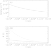 |
Fig. 3. Plasma density and magnetic field profiles obtained by the first fitting step: (A) Plasma density vs. height in Aschwanden’s model of the solar atmosphere. (B) Magnetic field vs. height in three models of the 1 August 2010 zebra with the gyro-harmonic numbers s = 26–30 (full line), s = 10–14 (dotted line), and s = 120–124 (dashed line). |
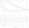 |
Fig. 4. Zebra model with the gyro-harmonic numbers s = 26–30. (A) Profiles of the upper-hybrid (dashed line) and s-harmonic of electron-cyclotron (full lines) frequencies obtained by the first fitting step. (B) Modeled radio spectrum with zebra stripes in the time interval 08:21:58–08:22:00 UT according to the zebra shown in Fig. 1 obtained by the first and second fitting steps. Large asterisks show frequencies of the observed zebra stripe used for the fitting, see the arrow in Fig. 1. Small diamonds show frequencies of other observed zebra stripes. |
Next, we carried out a further fitting (second fitting step) of the time variations of zebra-stripe frequencies considering global expansions or compressions of the part of the loop (Process A). For this purpose, we took the frequencies of the observed zebra stripe starting on 1330 MHz at 08:21:58 UT (see the arrow in Fig. 1) with the time resolution of 0.1 s. These frequencies are denoted in Fig. 4B with large asterisks. In each time instant, corresponding to the large asterisks, we fit the observed frequency (shown by large asterisks) by the small variation of the plasma density and magnetic field in the whole loop expressed by the factor V in the relations n(1 + V) and B(1 + V), where n and B are the plasma density and magnetic field obtained in the first fitting step. By this procedure, we obtained the model zebra stripe that fits the observed zebra-stripe frequencies denoted by large asterisks. Simultaneously, for the same factor, V, other zebra stripes were computed and shown in this figure by full lines as well. For comparison, the small diamonds in this figure show observed frequencies of other zebra stripes. Besides the very good fit of the zebra stripe denoted by large asterisks, other simulated zebra stripes partly deviate from the observed ones (small diamonds). We believe that this is due to the model assumptions regarding global expansion or compression of the loop, but not local effects; furthermore, the adopted density and magnetic field variations with height might have affected the result as well.
Now, for the purposes of general applications, we want to know how variations of the plasma density and magnetic field modify frequency variations of the zebra stripes in the same zebra, but considering different ranges of the gyro-harmonic number. For this purpose, we selected two ranges: one for s = 10–14, where s are lower than those in the case with s = 26–30, and the second one for s = 120–124, where s are higher than those in the case with s = 26–30. The applied procedure was the same as in the case with s = 26–30. The magnetic field profiles in these cases, obtained by the first fitting step, are shown in Fig. 3B and expressed by the relation (3) with the parameters: B0 = 42 000 G, Lb = 1720 km (dotted line) for s = 10–14 and B0 = 20.84 G, Lb = 7000 km (dashed line) for s = 120–124. The corresponding upper-hybrid and s-harmonic frequency profiles are shown in Figs. 5A and 6A, respectively. Similarly as in the case with s = 26–30, we made the second fitting step and the resulting zebra-stripe frequency profiles after this fitting step are shown in Figs. 5B and 6B.
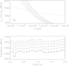 |
Fig. 5. Zebra model with the gyro-harmonic numbers s = 10–14. (A) Profiles of the upper-hybrid (dashed line) and s-harmonic of electron-cyclotron (full lines) frequencies obtained by the first fitting step. (B) Modeled radio spectrum with zebra stripes in the time interval 08:21:58–08:22:00 UT according to the zebra shown in Fig. 1 obtained by the first and second fitting steps. |
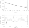 |
Fig. 6. Zebra model with the gyro-harmonic numbers s = 120–124. (A) Profiles of the upper-hybrid (dashed line) and s-harmonic of electron-cyclotron (full lines) frequencies obtained by the first fitting step. (B) Modeled radio spectrum with zebra stripes in the time interval 08:21:58–08:22:00 UT according to the zebra shown in Fig. 1 obtained by the first and second fitting steps. |
We go on to consider Fig. 4A and assume for a moment an increase of the plasma density in this figure. The s-harmonics of the gyro-cyclotron profiles are fixed and the upper-hybrid frequency profile shifts to higher frequencies and, thus the crossing points of the upper-hybrid and the s-harmonics of the gyro-cyclotron frequency profiles shift to lower heights where the upper-hybrid (zebra-stripe) frequency is higher. For the density decrease, the effect is opposite. Now, we increase the magnetic field only. Then, for the present values of parameters (s, n, and B in the zebra-stripe sources), the s-harmonics of the gyro-cyclotron frequency profiles shift to higher frequencies more than the upper-hybrid frequency profile and the crossing points of the upper-hybrid and the s-harmonics of the gyro-cyclotron frequency profiles shift to higher heights where the upper-hybrid (zebra-stripe) frequencies are lower. For the magnetic field decrease, the effect is opposite. We note that positions of zebra-stripe sources are changed in these cases. For Figs. 5A and 6A, these effects are similar as for Fig. 4A.
But, the zebra-stripe frequency variations in Figs. 4B, 5B and 6B were obtained by a change of both the density and magnetic field. Therefore, these variations are formed by two opposite effects and that is why this process is complex. The parameter V obtained in these cases is shown in Fig. 7. When we take here the cases for lower values of the gyro-harmonic number (s = 26–30 and 10–14) and compare the variations of V with the variations of the zebra-stripe frequencies in Figs. 4B and 5B we can see that an increase of the zebra-stripe frequencies corresponds to the positive values of V. Positive values of V mean that both the plasma density and magnetic field increase. In comparing this case with the above-mentioned cases, where only the plasma density increases or only the magnetic field increases, we can see that in this case, the effect of the density increase is stronger than that of the magnetic field increase. For high values of s (s = 120–124; as seen in Fig. 6B), the effect is opposite: the positive value of V corresponds to a decrease of the zebra-stripe frequency. Therefore, in this case, the effect of the magnetic field is stronger than that of the density. In any case, parameter V shows when the part of the loop with the zebra-stripe sources is compressed (V > 0) or expanded (V < 0).
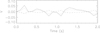 |
Fig. 7. Variations V in the multiplication factor (1 + V) of the plasma density and magnetic field vs. time (08:21:58–08:22:00 UT) in the zebra source corresponding to the variations of the zebra-stripe frequencies in three models with the gyro-harmonic numbers s = 26–30 (full line), s = 10–14 (dotted line), and s = 120–124 (dashed line). |
Our analysis shows that variations of the parameter V depend, in a complex way, on a positional shift of the region, where the DPR condition is fulfilled, and on gradients of the density and magnetic field profiles at times of density and magnetic field changes. Furthermore, it shows that the opposite sign of the parameter V for the cases with high and low values of s is connected with a contribution of the magnetic field to the upper-hybrid frequency for high and low values of s in the DPR condition. Namely, for high values of s, the upper-hybrid frequency practically does not depend on the magnetic field.
4. Simulation of the zebra pattern observed in the metric range on 21 June 2011
This zebra event was studied by Kaneda et al. (2018) and Yasnov (2021). Its radio spectrum is shown in Fig. 1C in the paper by Kaneda et al. (2018). Here, we consider a part of this zebra spectrum in the time interval 03:22:34.8–03:22:38.8 UT and 170–195 MHz range with five zebra stripes only. To simplify computations in the second fitting step, in the following simulations, we consider only the smoothed increase of the observed zebra-stripe frequencies between times 03:22:34.8 UT and 03:22:38.8 UT; thus neglecting deviations from this smoothed increase. To obtain the same time evolution of zebra-stripe frequencies in the model, we first fit the zebra-stripe frequencies at the starting time at 03:22:34.8 UT using Aschwanden’s density model and varying the magnetic field profile (first fitting step). The plasma density and the magnetic field at this time are shown in Fig. 8 by full lines. The magnetic field is described by the relation (3) with B0 = 4.02 G and Lb = 30 500 km. In accordance with Yasnov (2021) we took the gyro-harmonic numbers of the selected zebra stripes at 03:22:34.8 UT as s = 122–126; considering s = 131 for the zebra-stripe with the lowest frequency. As expected in continuous zebra stripes, the gyro-harmonic numbers in zebra stripes are the same during the whole interval of simulations (4 s). After the starting time (03:22:34.8 UT), owing to this reason, these gyro-harmonic numbers can differ from those presented by Yasnov (2021) in his Table 1. Moreover, to simplify the simulations, we did not take into account the linear dependance of R found in Yasnov (2021). We used the same model as for the zebra from 1 August 2010.
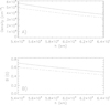 |
Fig. 8. Model plasma density (A) and magnetic field strength (B) at the starting (full lines) and ending (dashed lines) zebra times. |
Then, to express the smoothed time increase of the zebra-stripe frequencies between times 03:22:34.8 UT and 03:22:38.8 UT, we fit this frequency increase by an expansion of the loop only (Process A). In the resulting fit, the plasma density and magnetic field is multiplied by the time dependent factor (1 + V(t)), where V(t) = −0.0032 t and t is time in seconds (second fitting step). After four seconds, namely, at the ending time at 03:22:38.8 UT, the plasma density and magnetic field changed to values shown in Fig. 8 by dashed lines. Simultaneously, the upper-hybrid and s-harmonic of electron-cyclotron frequencies changed from values at 03:22:34.8 UT (see Fig. 9A) to those at 03:22:38.8 UT (see Fig. 9B). The crossing points of the upper-hybrid and s-harmonic of electron-cyclotron frequencies then determine the frequencies of the modelled zebra stripes, see Fig. 9C.
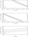 |
Fig. 9. Zebra case from 21 June 2011. (A) Model upper-hybrid (dashed line) and s-harmonic of electron-cyclotron (full lines) frequencies at the starting zebra time (03:22:34.8 UT). (B) Model upper-hybrid (dashed line), and s-harmonic of electron-cyclotron (full lines) frequencies at the ending zebra time (03:22:38.8 UT). (C) Modeled zebra stripes during the plasma density and magnetic field decrease (Process A) in the time interval 03:22:34.8–03:22:38.8 UT. |
In analyzing this zebra, Kaneda et al. (2018) reported a quasi-periodic modulation of zebra-stripe frequencies with the characteristic negative frequency drift of 3–8 MHz s−1 that they interpreted as the fast sausage mode waves propagating through the zebra source. Similar result was presented by Yasnov (2021), but with the inconsistent wave velocities derived from the estimated plasma density and magnetic field and those estimated from the frequency drift in the density models of the solar atmosphere.
Thus, we included these waves into our simulations (Process B). The wave wavelength (1370 km) was taken from the paper by Yasnov (2021). The amplitude of the wave at 03:22:34.8 UT was expressed by Yasnov (2021) through the density as A = δn/n = 0.00055 (Table 1 in Yasnov 2021) which corresponds the amplitude of variations of zebra-stripe frequencies δf ∼ 0.5 MHz.
First, we considered the Alfvén wave as a cause of these variations. We took the velocity of this wave as 57 km s−1 (the mean Alfvén velocity corresponding to the magnetic field and plasma densities in zebra-stripe sources). Then we varied its amplitude δB/B in order to fit the amplitude δf = 0.5 MHz derived from observations. The fit was obtained for δB/B = 0.0002. The resulting zebra-stripes in the interval 03:22:34.8–03:22:38.8 UT, together with δf, are shown in Figs. 10A,B, where δf is the difference between the zebra stripe with the lowest frequency in Figs. 9C and 10A. Thus, as can be seen, the inclusion of Process B into simulations made only a small modulation of the zebra-stripe frequencies.
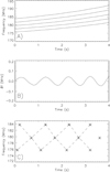 |
Fig. 10. Zebra case from 21 June 2011. (A) Zebra-stripe frequencies as in Fig. 9C, but with the δf variation caused by the Alfvén wave (amplitude δB/B = 0.0002, wavelength of 1370 km, and the Alfvén velocity 57 km s−1). (B) δf. C) Map of Δfn + 1 − Δfn, where Δfn = fn + 1 − fn, and fn is the frequency of the nth stripe numbered from the lowest frequency in the spectrum (part A). Asterisks mean maxima of these differences. Connecting dashed lines show the frequency drift. |
Then, knowing the time evolution of zebra-stripe frequencies, we used the same procedure as was used in the construction of Fig. 2C in the paper by Kaneda et al. (2018). In particular, at all time moments, we calculated second order differences between neighboring frequencies, that is, we calculated Δfn = fn + 1 − fn and then Δfn + 1 − Δfn, where fn is the frequency of the nth stripe numbered from the lowest frequency in the spectrum (Fig. 10A). The result is shown in Fig. 10C, where asterisks show maxima in this calculation and dashed line connect these maxima. Owing to only five modeled zebra-stripe frequencies, only the maxima at three frequencies can be presented. Nevertheless, Fig. 10C shows the cross-structure around the frequency 180 MHz. This cross-structure is similar to that of blue bands shown in Fig. 2C of the paper by Kaneda et al. (2018); we can see especially the cross-structure of blue bands at 03:22:45–03:22:55 UT and 160–180 MHz range in their Fig. 2C.
Similar computations we made for the magnetosonic wave, taking its velocity of 214 km s−1 (the mean magnetosonic velocity corresponding to the magnetic field and plasma densities in zebra-stripe sources and assumed coronal temperature 2 MK). In the analysis of the 1 August zebra, we found that the zebra-stripe frequencies are in the s = 120–124 case caused mainly by variations of the magnetic field. Therefore, once again we fit the amplitude δf = 0.5 MHz instead of direct application of the wave density amplitude derived by Yasnov (2021). The fit for variations of δf = 0.5 MHz was obtained for the amplitude of the magnetosonic wave, δn/n = δB/B = 0.0015. The zebra stripes, δf, and the cross-structure around 180 MHz are shown in Fig. 11. As seen here, Figs. 10C and 11C are very similar.
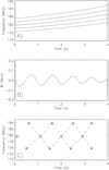 |
Fig. 11. Zebra case from 21 June 2011. (A) Zebra-stripe frequencies as in Fig. 9C, but with the δf variation caused by the magnetosonic wave (amplitude δn/n = δB/B = 0.0015, wavelength of 1370 km, and the velocity 214 km s−1). (B) δf. (C) Map of Δfn + 1 − Δfn, where Δfn = fn + 1 − fn, and fn is the frequency of the nth stripe numbered from the lowest frequency in the spectrum (part A). Asterisks mean maxima of these differences. Connecting dashed lines show the frequency drift. |
The most important fact, presented in Figs. 10C and 11C, is the time shift of maxima (asterisks), when we compare them at neighboring frequencies. This shift indicates the frequency drift in both these cases is about 8 MHz s−1 (see dashed lines), in agreement with Kaneda et al. (2018). However, as we can see, the velocities of the present waves differ considerably from those derived in Kaneda et al. (2018) (3000–8000 km s−1).
5. Discussion and conclusions
We successfully modeled two zebras: one from the decimetric range observed at 1 August 2010 and second one from the metric range observed at 21 June 2011. While the 1 August 2010 zebra was modeled only based on variations of the plasma density and magnetic field in the expanding and compressing loop, where the zebra-stripe sources were located, in the 21 June 2011 zebra the variations of zebra-stripe frequencies are modeled by an expansion of the loop together with the Alfvén or magnetosonic waves propagating along the loop. Small deviations of modeled zebra stripes from those observed are given by deviations of the used model from real conditions. These simulations confirm that DPR model correctly describes the analyzed zebras.
In our modeling we found that increasing the density or decreasing the magnetic field in the part of the loop, where zebra-stripe sources are located, the zebra stripes are shifted to higher frequencies, and vice versa, namely, decreasing the density or increasing the magnetic field the zebra stripes are shifted to lower frequencies.
We found that variations of zebra-stripe frequencies are generally the result of variations of both the magnetic field and wave density, except for the propagating Alfvén wave where only the magnetic field plays a role. In the case of the zebra from 21 June 2011, we confirmed that small variations of distances between neighboring zebra-stripe frequencies can be explained by waves propagating along the loop as proposed by Yasnov (2021).
Furthermore, we showed that in the assumed Aschwanden’s density model of the solar atmosphere the zebra observed in the decimetric range (the 1 August 2010 zebra) can be modeled in a broad range of the gyro-harmonic numbers. On the other hand, the zebra in the metric range (the 21 June 2011 zebra) in this density model can be modeled only for high values of the gyro-harmonic numbers; this is in agreement with those found by Yasnov (2021). In addition, we found that for simulation of the 21 June 2011 zebra with lower values of the gyro-harmonic numbers, the density model with a faster decrease of the density in dependance on height is needed.
We found that there are differences in the magnetic field in zebra sources with different ranges of s. For small values of s of the zebra stripes, the magnetic field in the zebra-stripe sources is higher and changes faster than for high values of s. Thus, for s > 100 the magnetic field in all zebra-stripe sources is low and nearly constant.
In the zebra from 1 August 2010, the mean magnetic field in the zebra-stripe sources in the case for s = 10–14 is about 40 G, for s = 26–30 is about 15 G, and for s = 120–124 is about 4 G; see Fig. 3B for the height 1.2 × 10⁴ km. For comparison, in the model from Dulk & McLean (1978), the magnetic field at the same height is about 100 G.
Similarly, in the zebra from 21 June 2011 for s = 122–126, this magnetic field is about 0.6 G (see Fig. 8B at the height 5.9 × 10⁴ km). For comparison, in the model by Dulk & McLean (1978) the magnetic field at the same height is about 20 G, and in the model by Gopalswamy et al. (1986) is 3.6–8.6 G. Thus, in both zebra cases, the simulated magnetic field is lower than that in the models by Dulk & McLean (1978) and Gopalswamy et al. (1986).
In the case of the 21 June 2011 zebra, we confirmed the very high values of the gyro-harmonic number (s = 122–126), as presented by Yasnov (2021). In the simulations, we considered the velocity of the Alfvén or magnetosonic waves as follows from the model values of the magnetic field, plasma density, and assumed coronal temperature. Although these values are much smaller than those derived by Kaneda et al. (2018), we obtained a similar frequency drift shown in Figs. 10C and 11C as in Fig. 2C in the paper by Kaneda et al. (2018). Namely, in our model this frequency drift is only partly caused by the wave velocity. This is mainly owing to a decrease of the plasma density and magnetic field in the loop. This result also explains quite different velocities of the magnetosonic wave derived from plasma parameters and from the frequency drift and density model of the solar atmosphere as presented by Yasnov (2021).
As noted in introduction, the computations of DPR instability show that its growth rate decreases with an increase of the gyro-harmonic number, s. However, a simulation of the 21 June 2011 zebra confirmed high values of s, in agreement with (Yasnov 2021). In this case, it means that the loss-cone distribution of superthermal electrons with the appropriate type that is necessary for the zebra generation was formed in the region with high values of s. However, high values of s also mean that the magnetic field in the zebra-stripe sources is nearly constant. This might be related to the fact that coronal loops tend to be only slightly (∼30%) wider at their midpoints than at their footpoints and the cross-section has an approximately circular shape (Klimchuk 2000), namely, the change of the magnetic field field along the loop is relatively small. In four cases (three with s = 10–14, 26–30 and 120–124 for the 1 August 2010 zebra) and with s = 114–131, for all observed zebra stripes in the 21 June 2011 zebra, we took whole frequency bands of analyzed zebras and using our model, we determined for them the height intervals together with the corresponding intervals of the magnetic field (see Table 1). Using these magnetic field values, we calculated the relative change of the magnetic field in these height intervals (last column in Table 1). As seen here, for the 1 August 2010 zebra, an increase of s leads to a decrease of this relative change from 50% to 15%. For the 21 June 2011 zebra it is 36%. When we compare these with the aforementioned value of the loop (∼30%), then a rough agreement can be found for s greater than about 30 for the 1 August 2010 zebra and, perhaps, for s found for the 21 June 2011 zebra. However, we note that the estimations presented in Table 1 are only for the part of the loop where zebra-stripe sources are located.
Parameters of the 1 August 2010 and 21 June 2011 zebras.
This relative low change of the loop cross-section along loops (Klimchuk 2000) only partly supports the high values of the gyro-harmonic number in observed zebras. Therefore, a further detailed analysis of the growth rates of DPR instability for high values of s is need, which considers different distributions of superthermal electrons, especially those with the loss-cones close to 90 degrees. Simultaneously, a search ought to be carried out to find regions in the solar flare atmosphere with a high ratio for the plasma and electron-cyclotron frequencies and with proper conditions for zebra generation.
Acknowledgments
The author thanks the referee for useful comments that improved the paper. He also acknowledges support from the project RVO-67985815 and GA ČR grants 20-09922J, 20-07908S, 21-16508J, and 22-34841S.
References
- Aschwanden, M. J. 2002, Space Sci. Rev., 101, 1 [Google Scholar]
- Benáček, J., Karlický, M., & Yasnov, L. V. 2017, A&A, 598, A106 [NASA ADS] [CrossRef] [EDP Sciences] [Google Scholar]
- Chen, B., Bastian, T. S., Gary, D. E., & Jing, J. 2011, ApJ, 736, 64 [NASA ADS] [CrossRef] [Google Scholar]
- Chernov, G. P. 2006, Space Sci. Rev., 127, 195 [Google Scholar]
- Chernov, G. 2011, Fine Structure of Solar Radio Bursts, Astrophysics and Space Science Library (Heidelberg: Springer) [Google Scholar]
- Dulk, G. A., & McLean, D. J. 1978, Sol. Phys., 57, 279 [CrossRef] [Google Scholar]
- Gopalswamy, N., Thejappa, G., Sastry, C. V., & Tlamicha, A. 1986, Bull. Astron. Inst. Czech., 37, 115 [NASA ADS] [Google Scholar]
- Jiřička, K., & Karlický, M. 2008, Sol. Phys., 253, 95 [CrossRef] [Google Scholar]
- Kaneda, K., Misawa, H., Iwai, K., et al. 2018, ApJ, 855, L29 [Google Scholar]
- Karlický, M., & Yasnov, L. 2015, A&A, 581, A115 [NASA ADS] [CrossRef] [EDP Sciences] [Google Scholar]
- Karlický, M., & Yasnov, L. V. 2018, ApJ, 867, 28 [CrossRef] [Google Scholar]
- Karlický, M., & Yasnov, L. 2020, A&A, 638, A22 [EDP Sciences] [Google Scholar]
- Karlický, M., & Yasnov, L. V. 2021, A&A, 646, A179 [NASA ADS] [CrossRef] [EDP Sciences] [Google Scholar]
- Klimchuk, J. A. 2000, Sol. Phys., 193, 53 [NASA ADS] [CrossRef] [Google Scholar]
- Kuijpers, J. M. E. 1975, PhD Thesis, Utrecht, Rijksuniversiteit, Doctor in de Wiskunde en Natuurwetenschappen Dissertation, 1975, 72 [Google Scholar]
- Kuijpers, J. 1980, in Radio Physics of the Sun, eds. M. R. Kundu, & T. E. Gergely, IAU Symp., 86, 341 [Google Scholar]
- Mollwo, L. 1983, Sol. Phys., 83, 305 [Google Scholar]
- Mollwo, L. 1988, Sol. Phys., 116, 323 [NASA ADS] [Google Scholar]
- Slottje, C. 1981, Atlas of fine structures of dynamics spectra of solar type IV-dm and some type II radio bursts (The Netherlands: Dwingeloo Observatory) [Google Scholar]
- Tan, B., Yan, Y., Tan, C., Sych, R., & Gao, G. 2012, ApJ, 744, 166 [Google Scholar]
- Tan, B., Tan, C., Zhang, Y., Mészárosová, H., & Karlický, M. 2014, ApJ, 780, 129 [Google Scholar]
- Winglee, R. M., & Dulk, G. A. 1986, ApJ, 307, 808 [Google Scholar]
- Yasnov, L. V. 2021, Sol. Phys., 296, 139 [NASA ADS] [CrossRef] [Google Scholar]
- Yasnov, L. V., & Karlický, M. 2020, Sol. Phys., 295, 96 [Google Scholar]
- Yasnov, L. V., Karlický, M., & Stupishin, A. G. 2016, Sol. Phys., 291, 2037 [CrossRef] [Google Scholar]
- Zheleznyakov, V. V., & Zlotnik, E. Y. 1975, Sol. Phys., 44, 461 [Google Scholar]
- Zlotnik, E. Y. 2013, Sol. Phys., 284, 579 [NASA ADS] [CrossRef] [Google Scholar]
All Tables
All Figures
|
Fig. 1. Dynamic radio spectrum with the zebra observed on 1 August 2010 by the Ondřejov radiospectrograph (Jiřička & Karlický 2008). The arrow shows the zebra stripe chosen for the zebra-stripe fitting. |
| In the text | |
|
Fig. 2. Schema of the model. |
| In the text | |
|
Fig. 3. Plasma density and magnetic field profiles obtained by the first fitting step: (A) Plasma density vs. height in Aschwanden’s model of the solar atmosphere. (B) Magnetic field vs. height in three models of the 1 August 2010 zebra with the gyro-harmonic numbers s = 26–30 (full line), s = 10–14 (dotted line), and s = 120–124 (dashed line). |
| In the text | |
|
Fig. 4. Zebra model with the gyro-harmonic numbers s = 26–30. (A) Profiles of the upper-hybrid (dashed line) and s-harmonic of electron-cyclotron (full lines) frequencies obtained by the first fitting step. (B) Modeled radio spectrum with zebra stripes in the time interval 08:21:58–08:22:00 UT according to the zebra shown in Fig. 1 obtained by the first and second fitting steps. Large asterisks show frequencies of the observed zebra stripe used for the fitting, see the arrow in Fig. 1. Small diamonds show frequencies of other observed zebra stripes. |
| In the text | |
|
Fig. 5. Zebra model with the gyro-harmonic numbers s = 10–14. (A) Profiles of the upper-hybrid (dashed line) and s-harmonic of electron-cyclotron (full lines) frequencies obtained by the first fitting step. (B) Modeled radio spectrum with zebra stripes in the time interval 08:21:58–08:22:00 UT according to the zebra shown in Fig. 1 obtained by the first and second fitting steps. |
| In the text | |
|
Fig. 6. Zebra model with the gyro-harmonic numbers s = 120–124. (A) Profiles of the upper-hybrid (dashed line) and s-harmonic of electron-cyclotron (full lines) frequencies obtained by the first fitting step. (B) Modeled radio spectrum with zebra stripes in the time interval 08:21:58–08:22:00 UT according to the zebra shown in Fig. 1 obtained by the first and second fitting steps. |
| In the text | |
|
Fig. 7. Variations V in the multiplication factor (1 + V) of the plasma density and magnetic field vs. time (08:21:58–08:22:00 UT) in the zebra source corresponding to the variations of the zebra-stripe frequencies in three models with the gyro-harmonic numbers s = 26–30 (full line), s = 10–14 (dotted line), and s = 120–124 (dashed line). |
| In the text | |
|
Fig. 8. Model plasma density (A) and magnetic field strength (B) at the starting (full lines) and ending (dashed lines) zebra times. |
| In the text | |
|
Fig. 9. Zebra case from 21 June 2011. (A) Model upper-hybrid (dashed line) and s-harmonic of electron-cyclotron (full lines) frequencies at the starting zebra time (03:22:34.8 UT). (B) Model upper-hybrid (dashed line), and s-harmonic of electron-cyclotron (full lines) frequencies at the ending zebra time (03:22:38.8 UT). (C) Modeled zebra stripes during the plasma density and magnetic field decrease (Process A) in the time interval 03:22:34.8–03:22:38.8 UT. |
| In the text | |
|
Fig. 10. Zebra case from 21 June 2011. (A) Zebra-stripe frequencies as in Fig. 9C, but with the δf variation caused by the Alfvén wave (amplitude δB/B = 0.0002, wavelength of 1370 km, and the Alfvén velocity 57 km s−1). (B) δf. C) Map of Δfn + 1 − Δfn, where Δfn = fn + 1 − fn, and fn is the frequency of the nth stripe numbered from the lowest frequency in the spectrum (part A). Asterisks mean maxima of these differences. Connecting dashed lines show the frequency drift. |
| In the text | |
|
Fig. 11. Zebra case from 21 June 2011. (A) Zebra-stripe frequencies as in Fig. 9C, but with the δf variation caused by the magnetosonic wave (amplitude δn/n = δB/B = 0.0015, wavelength of 1370 km, and the velocity 214 km s−1). (B) δf. (C) Map of Δfn + 1 − Δfn, where Δfn = fn + 1 − fn, and fn is the frequency of the nth stripe numbered from the lowest frequency in the spectrum (part A). Asterisks mean maxima of these differences. Connecting dashed lines show the frequency drift. |
| In the text | |
Current usage metrics show cumulative count of Article Views (full-text article views including HTML views, PDF and ePub downloads, according to the available data) and Abstracts Views on Vision4Press platform.
Data correspond to usage on the plateform after 2015. The current usage metrics is available 48-96 hours after online publication and is updated daily on week days.
Initial download of the metrics may take a while.