| Issue |
A&A
Volume 661, May 2022
The Early Data Release of eROSITA and Mikhail Pavlinsky ART-XC on the SRG mission
|
|
|---|---|---|
| Article Number | A24 | |
| Number of page(s) | 11 | |
| Section | Stellar atmospheres | |
| DOI | https://doi.org/10.1051/0004-6361/202141020 | |
| Published online | 18 May 2022 | |
The corona – chromosphere connection studied with simultaneous eROSITA and TIGRE observations★
Hamburger Sternwarte, Universität Hamburg,
Gojenbergsweg 112,
21029
Hamburg, Germany
e-mail: This email address is being protected from spambots. You need JavaScript enabled to view it.
Received:
8
April
2021
Accepted:
31
May
2021
Abstract
Stellar activity manifests itself in a variety of different phenomena, some of which we can measure as activity tracers from different atmospheric layers of the star, typically at different wavelengths. Stellar activity is furthermore inherently time variable, therefore simultaneous measurements are necessary to study the correlation between different activity indicators. In this study we compare X-ray fluxes measured within the first all-sky survey conducted by the extended ROentgen Survey with an Imaging Telescope Array (eROSITA) instrument on board the Spectrum-Roentgen-Gamma observatory to Ca II H&K excess flux measurements RHK+, using observations made with the robotic TIGRE telescope. We created the largest sample of simultaneous X-ray and spectroscopic Ca II H&K observations of late-type stars obtained so far, and in addition, previous measurements of Ca II H&K for all sample stars were obtained. We find the expected correlation between our log(LX/Lbol) to log(RHK+) measurements, but when the whole stellar ensemble is considered, the correlation between coronal and chromospheric activity indicators does not improve when the simultaneously measured data are used. A more detailed analysis shows that the correlation of log(LX/Lbol) to log(RHK+) measurements of the pseudo-simultaneous data still has a high probability of being better than that of a random set of non-simultaneous measurements with a long time baseline between the observations. Cyclic variations on longer timescales are therefore far more important for the activity flux-flux relations than short-term variations in the form of rotational modulation or flares, regarding the addition of “noise” to the activity flux-flux correlations. Finally, regarding the question of predictability of necessarily space-based log (LX/Lbol) measurements by using ground-based chromospheric indices, we present a relation for estimating log (LX/Lbol) from RHK+ values and show that the expected error in the calculated minus observed (C-O) log (LX/Lbol) values is 0.35 dex.
Key words: stars: activity / stars: chromospheres / stars: coronae / stars: late-type / X-rays: stars
Full Table 3 is only available at the CDS via anonymous ftp to cdsarc.u-strasbg.fr (130.79.128.5) or via http://cdsarc.u-strasbg.fr/viz-bin/cat/J/A+A/661/A24
© ESO 2022
1 Introduction
Magnetic stellar activity manifests itself in a zoo of phenomena, originating in various layers of the stellar atmosphere. This is observable throughout the electromagnetic spectrum. In the optical, photometric variability (e.g. Suárez Mascareño et al. 2016) is observed that is attributed to star spots, which are located in the stellar photospheres and rotate in and out of the field of view. Activity phenomena of the chromosphere and transition region are frequently studied using several optical and ultraviolet spectral lines (Baliunas et al. 1996; Wright et al. 2004). Finally, the tenuous and hot coronal gas can be observed at X-ray wavelengths (Güdel 2004; Robrade & Schmitt 2005).
All these different tracers of magnetic activity are ultimately thought to be powered by a stellar dynamo, operating in the interiors of stars with outer convection zones. Chromospheric emission lines additionally show a so-called basal level that may be caused by energy dissipation of acoustic waves in the chromosphere and perhaps the transition region (Rutten et al. 1991; Wedemeyer et al. 2004). A comparable basal level has not been observed in X-rays (Stepien & Ulmschneider 1989; Schrijver et al. 1992). Although a minimum flux observed by Schmitt (1997) also exists, it is more than two magnitudes higher than the expected value from acoustic heating (Stepien & Ulmschneider 1989). Instead, it coincides with the X-ray flux level from solar coronal holes, which represents the minimum observed flux from the solar corona.
Optical spectral and photometric activity tracers have been studied in time-series observations of individual stars, which revealed activity cycles (Hempelmann et al. 2006), stellar rotation periods (Suárez Mascareño et al. 2016; Schöfer et al. 2019; Fuhrmeister et al. 2019), and flares (Fuhrmeister et al. 2008), for instance. These studies have allowed analysing the relation between different activity tracers, and they showed that the tracers tend to be well correlated. However, many authors also find that this is not necessarily true for all activity tracers all the time. For example, Gomes da Silva et al. (2011) found in a study of M dwarfs that the emission in the Hα and the Ca II H&K lines need not correlate in lower-activity stars, while this is the case for more active stars. They therefore recommended using either the Ca II H&K lines or the Na ID lines as a proxy for the activity level in M dwarfs. Nonetheless, there may be good correlations between the Hα and the Ca II H&K lines for individual stars (e.g. Robertson et al. 2016). Considering earlier type stars as well, Díaz et al. (2007) concluded from a study of F6 to M 5.5 stars that Na I D can only be used as activity indicators for the most active stars.
Using an ensemble of diagnostics, activity throughout the stellar atmosphere can be studied. For example, Walkowicz & Hawley (2009) analysed the correlation between the emission in the Ca II H&K, Hα, and Mg II ultraviolet lines and the X-ray flux in a sample of M 3 stars. These indicators trace layers of the stellar atmosphere with increasing height. Walkowicz & Hawley (2009) found a good correlation between fluxes originating in the lower and upper chromosphere as traced by the Ca II H&K and Hα lines, again only for active stars. In stars with a high or intermediate activity level, power-law relations were found between the X-ray coronal and optical chromospheric line tracers.
Comparisons of the X-ray flux and the Ca II H&K excess emission were also performed for more solar-type stars (Schrijver 1983; Mittag et al. 2018). The power-law relation between the chromospheric CaII H&K emission and the coronal X-ray flux holds over four orders of magnitude in X-ray flux; the Sun also follows this relation during its activity cycle. In a similar study, Martínez-Arnáiz et al. (2011a) deduced power-law dependences between several chromospheric and X-ray indicators using a spectral subtraction technique that eliminates photospheric and basal contributions in their simultaneous chro-mospheric data. They derived flux−flux relations for the Hα, CaII H&K, and CaII IRT lines and the X-ray flux using 298 F- to M-type stars, including some younger stars. He et al. (2019) found a similar correlation between log (LX/Lbol) and log (LHα/Lbol) for 484 F- to M-type stars.
The correlation between chromospheric and coronal fluxes extends over many orders of magnitude and hence is quite striking, but it shows considerable scatter, the reasons for which are unclear. A possible explanation clearly is that the vast majority of data sets does not provide simultaneous chromospheric and coronal measurements, and the chromosphere and corona of the same star are compared, but at very different times and therefore at possibly different activity levels. In an attempt to address this issue, Schrijver et al. (1992) studied a small sample of stars for which nearly simultaneous measurements of the fluxes in the Mg II h&k lines (with the IUE satellite), of the broad-band soft X-ray flux (with the EXOSAT satellite), and the Ca II H&K core emission as determined from Mount Wilson S-indices were available. Schrijver et al. (1992) reported that the scatter is reduced when near-simultaneous data are used and that the remaining scatter can be entirely attributed to uncertainties in the instrumental calibration and flux conversion factors.
To increase the sample size and improve the temporal alignment, we used our robotic TIGRE telescope to obtain the largest sample of (pseudo-)simultaneous, high-resolution optical spectra of stars observed at X-ray wavelengths so far in the framework of the first all-sky survey by the extended ROentgen Survey with an Imaging Telescope Array (eROSITA). Because we have non-simultaneous data as well, we can analyse the effect of the simultaneity on the power-law distribution connecting the X-ray flux and chromospheric tracers. We wish to study in particular whether part of the scatter in this relation is due to non-simultaneous data and explore in this context how well log (LX/Lbol) can be predicted by chromospheric indicators measured from the ground.
2 Stellar sample and observations
In this section we first describe our stellar sample, followed by an overview of our X-ray eROSITA and optical TIGRE observations. We also provide a description of the applied scheduling procedures to obtain a pseudo-simultaneous data set and characterise these data. Finally, we introduce the chromospheric activity indicator  .
.
Basic properties of the sample stars.
2.1 Stellar sample
To accomplish our goals, we need a sample of stars that is as equally distributed in spectral type and activity level as possible, with a preferably small fraction of low-activity stars without X-ray detection by eROSITA and bright enough to be observed by the TIGRE telescope; a representative volume-limited sample is therefore not the best choice. We therefore constructed a sample of 404 stars with spectral types between M and F indicated by a colour constraint1 of 0.24 ≤ B−V ≤ 1.5 mag (see Table 1). From these, we selected all optically bright (V ≤ 9.5 mag) stars, which must additionally be located in the western galactic hemisphere at galactic longitudes between 180° and 360°, where eROSITA data is available to us. Moreover, we applied an individual distance cut for spectral type groups provided in Table 1. The distance cut was larger for stars with a detection by the ROSAT satellite (count rate in excess of 0.01 ctss−1) compared to stars without. Resolvable binaries were excluded from our sample. However, we included 48 binary candidates covering spectroscopic binaries or RS CVn systems, which are unresolved by eROSITA and TIGRE. We discuss these stars further in Sects. 3.1 and 3.4.
Thus our sample is a compromise between a volume-limited sample and a more active sample in which we expect more eROSITA detections. The sample has a slight bias on solar-type and earlier stars because the fainter later stars require far longer observation times in the optical.
2.2 eROSITA data
The eROSITA X-ray telescope is the main instrument on board the Spectrum-Roentgen-Gamma satellite (SRG, Predehl et al. 2021). The SRG is carrying out a total of eight all-sky surveys in the 0.2–8 keV range and performs the first ever systematic all-sky survey in the 2.4–8 keV X-ray band. Thus, the eROSITA survey complements the ROSAT all-sky survey (RASS) carried out in 1990 in the 0.1–2.4 keV energy range, and significantly surpasses it in terms of sensitivity, spatial, and spectral resolution.
For our study we only used results of the first of the eight eROSITA all-sky surveys, using the processing results of the eSASS pipeline (currently version 946); a detailed description of this software and the algorithms we used is given by Brunner et al. (2022). Briefly, the eSASS system performs source detection and creates X-ray catalogues for each sky tile with a size of 3.6° × 3.6° in which neighbouring sky tiles overlap. The X-ray sources in the individual tiles are then merged into one large catalogue. Duplications in the overlap regions were removed and astrometric corrections were applied. These catalogue count rates are fiducial count rates that would be obtained if the source in question were observed by all seven eROSITA telescopes on-axis; we note that during the survey, the off-axis angle changes all the time, and furthermore, not all seven telescopes may deliver useful data at all times due to calibration activities or malfunction. The software performs source detection in the energy bands 0.2−0.6 keV, 0.6−2.3 keV, and 2.3−5.0 keV and also considers a total band 0.2−5.0 keV. Because stellar coro-nae tend to be rather soft X-ray emitters, most of our sample stars have no counts, or counts that agree with zero counts in the highest-energy band. We therefore only used the energy bands 0.2−0.6 keV and 0.6−2.3 keV for our analysis.
Furthermore, the measured count rates in the two lower-energy bands show a high degree of correlation. We therefore used the summed count rates in the 0.2-2.3 keV band and applied an energy conversion factor (ECF) of 0.9 ×10⁻¹² erg cm−2 cnt−1 to convert measured count rates into inferred energy fluxes. We note that this ECF is appropriate for a thermal plasma emission with a temperature of 1 keV and an absorption column of 3 × 1019 cm−2. No attempt was made to apply individual conversion factors to individual sources based on their X-ray spectra because many of our sources are too weak to meaningfully fit a coronal spectral model. We estimate that the errors of our preliminary calculations lead to flux errors of about 10 to 20%. This is supported by simulations with thermal models of a single-temperature coronal plasma and the eROSITA response function, which show that the ECF varies by about 10% for coronal temperature changes in the range between 0.2 keV to 1.0 keV.
To further bolster our error estimates, we compared the tabulated fluxes to ROSAT fluxes obtained with the hardness-ratio-dependent conversion factor given by Schmitt et al. (1995), which is based on coronal spectral models. The ROSAT fluxes calculated in this way are about 25% higher than their eROSITA counterparts. This can mostly be attributed to the softer ROSAT energy band, which leads to systematically higher fluxes by 15% using standard coronal models.
Proceeding in this fashion, we identified X-ray counterparts for 343 of our sample stars in eRASS1 and 320 in the RASS catalogue (2RXS) by Boller et al. (2016), see Table 2. We used a search radius of 18 arcsec for eRASS1 and a search radius of 40 arcsec for the ROSAT catalogue. We estimate our completeness to be more than 95%, with a marginal number of by-chance-detections.
Thirty-eight stars have X-ray detections in eRASS1 but not in 2RXS. About half of them have low count rates at the detection threshold of eRASS1, demonstrating the higher sensitivity of eROSITA compared with ROSAT. Boller et al. (2016) stated a detection limit in 2RXS of 10−13 erg cm−2 s−1. The X-ray emission of 18 of these 38 stars without a ROSAT detection is below that value. Another 7 stars without a ROSAT detection have flux values below 2 × 10⁻¹³ erg cm−2 s−1. Of the remaining stars, 3 have counts in the hardest band and may therefore have undergone flares during the eROSITA observation. The rest may be explained either by long-term activity variation (cycles) or spurious detections.
Finally, we converted the measured X-ray fluxes into X-ray luminosities using parallaxes from Gaia DR2 (Gaia Collaboration 2018) and HIPPARCOS (van Leeuwen 2007) and calculated the bolometric luminosities of our stars by interpolating the values given by Pecaut & Mamajek (2013)2. To provide an overview of the properties of our stellar sample, we show in Fig. 1 a Hertzsprung-Russell (HR) diagram of a sub-sample of our program stars, defined in Sect. 2.3.1 as a valid sample (all stars with an X-ray counterpart, but excluding earlier-type stars, sub-giants, and noisy data). Figure 1 shows the smooth distribution of stars in B−V as well as their X-ray properties characterised by their eROSITA-measured log (LX/Lbol) values.
Observational properties.
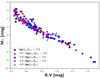 |
Fig. 1 HR diagram of a sub-sample of our stars defined as a valid sample in Sect. 2.3.1 that also shows the X-ray properties of these stars. |
2.3 TIGRE data
We used our robotic TIGRE telescope to obtain high-resolution (R ≈ 20000) optical spectra of our sample stars. TIGRE is a 1.2 m telescope located in central Mexico at the La Luz Observatory of the University of Guanajuato. The telescope is fibre-coupled to an échelle spectrograph with a wavelength coverage from 3800 to 8800 Å. From the 2D échelle images, 1D science spectra are obtained via a reduction pipeline; a detailed description of the TIGRE facility is given by Schmitt et al. (2014).
The spectral range of TIGRE is divided into two arms. The blue arm covers the spectral range shortwards of 5800 Å, and the red arm covers the range longwards of 5900 Å, extending up to about 8800 Å. Thus, the blue arm covers the Ca II H&K lines, which we focus upon in this paper, while the red arm contains the Hα and the Ca II IRT lines, which also provide chromospheric diagnostics. Along with the 1D science spectra, the reduction pipeline also determines activity indices, and the instrumental Ca II H&K index can be converted into the Mount Wilson Observatory S-index (SMWO) using the relation by Mittag et al. (2016) to ensure comparability with other measurements.
2.3.1 Characterisation of the pseudo-simultaneous data
The X-ray measurements span some time because eROSITA scans the sky along great circles with a scan period of 4 h; thus any source stays within the eROSITA field of view for at most 40 s per scan. The scanned great circles move along the plane of the ecliptic with a (somewhat variable) rate of about 1° per day, so that a source near the plane of the ecliptic is visited six times within 24 h, while sources at higher ecliptic latitude are observed longer. We define the middle of the eROSITA observations as the average of time between the first scan and last scan (even if at that time the star was actually not being scanned). To provide a few numbers, the longest scan period of eROSITA among our stars is 6.5 days, and about 20 stars have scan elapsed times longer than two days. For the purposes of this paper, it is essential to obtain spectral observations pseudo-simultaneously with the eROSITA X-ray measurements. In the context of this study, we consider all optical spectra taken within three days before or after the start or stop of the X-ray observation as pseudo-simultaneous.
Next, the great circles scanned by eROSITA are more or less 90° away from the Sun, and therefore eROSITA can never observe in the anti-Sun direction that is normally favoured by optical observers. As a consequence, TIGRE observations have to take place either shortly after sunset or just prior to sunrise, and the allowed observing window can be as short as 24 h. Scheduling these (pseudo-)simultaneous observations therefore is a challenge and certainly a task ideal for robotic telescopes. For reference, we also obtained non-simultaneous spectra of our program stars.
The TIGRE exposure time is set to obtain a signal-to-noise ratio (S/N) of 100 at 6000 Å, but for spectra to be usable for Ca II H&K studies, we demand a posteriori a mean S/N greater than 20 in the blue arm, which we found necessary to compute a meaningful Ca II H&K index. During the eRASS1 data taking, our pseudo-simultaneous TIGRE observation program therefore led to 550 usable spectra for a total of 312 stars, see Table 2.
Moreover, when we also consider the non-simultaneous observations of the sample stars, we have 9 or more spectra for the majority of stars, and for a sub-sample of 15 stars, we even have 100 or more spectra. Unfortunately, for 10 faint and very late-type stars, no spectra were obtained with usable Ca II H&K data. For another 15 of the faintest stars, we have only one or two usable spectra.
In Fig. 2 we show the distribution of the temporal offset between the TIGRE observations and the time centre of the eROSITA observation for the usable pseudo-simultaneous TIGRE observations. The time centre of the eROSITA observations is defined as the mid-time between the first and last eROSITA scan as explained above. Two peaks can clearly be distinguished in the distribution, separated by about two days, but Fig. 2 shows that our goal of reaching pseudo-simultaneous observations has been accomplished quite well.
The number of stars with eROSITA X-ray measurements and pseudo-simultaneous TIGRE data that lie in the colour range B−V > 0.44 mag (to ensure that the conversion relation to  and
and  values is valid; cf. Sect. 2.3.2) is 203. From this sample we excluded 20 stars that are outliers in our HR diagram (most of them are probably sub-giants) or are outliers in
  , which normally is found for stars with very low surface gravities or peculiar metallicity values. This selection leaves us with 183 stars, which we call the valid sample in the following.
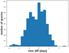 |
Fig. 2 Number of spectra taken by TIGRE for a certain offset between the middle of the eROSITA observation and the time of the TIGRE observations for pseudo-simultaneous data. |
2.3.2 Conversion into  and
and 
The so-called Mount Wilson S-index (SMWO) as defined by Wilson (1978) is a purely instrumental index that must be calibrated to obtain physical quantities and allow comparisons between stars of different spectral type. Furthermore, it contains both chromospheric and photospheric non-activity-related contributions, so that we have to remove the latter, which depend on stellar effective temperature or colour, respectively.
Comparisons between stars with different spectral types become possible by the introduction of the  index (empirically defined by Hartmann et al. 1984; Noyes et al. 1984). This is the ratio of the chromospheric Ca II H&K line fluxes and the bolometric flux. Mittag et al. (2013) revisited the S-index calibration, taking advantage of synthetic PHOENIX models (Hauschildt et al. 1999), and introduced an additional index,
  , that differs from
  by the subtraction of a basal activity level from the Ca II H&K line flux. This basal activity level is thought to be caused by heating by acoustic waves that are produced by turbulent convective motions and deposit their mechanical energy in the chromosphere (Schrijver 1995; Wedemeyer et al. 2004). Although previous studies did not introduce the term
  , the technique of identifying and eventually subtracting this nonmagnetic heating from the line flux has had a long tradition (see e.g. Schrijver 1987; Mathioudakis & Doyle 1992).
We first converted STIGRE into the SMWO index using the relation by Mittag et al. (2016) and then into  using two relations, first, the “classical” relation given by Noyes et al. (1984), and, second, the more recent relation published by Mittag et al. (2013). The latter also allows conversion into the
  index. The relations by Noyes et al. (1984) and Mittag et al. (2013) are only defined for stars within the colour ranges 0.44 < B−V < 0.9 and 0.44 < B−V < 1.6, respectively. Unfortunately, 65 earlier-type program stars (see Table 1) are outside either range. We excluded them from the conversion for the time being. Late-type stars with B−V colour larger than 0.9, that is, beyond the range of validity defined by Noyes et al. (1984), were not discarded for comparison purposes, with the relation extrapolated to these B−V values.
We compare the Noyes et al. (1984) and Mittag et al. (2013) conversions into  in Fig. 3. The relation proposed by Mittag et al. (2013) leads to systematically higher
  values, and the difference slightly grows toward the most active stars. Because the two relations are derived from a different ansatz, some discrepancy may be expected. With the available data, it cannot be decided which relation is better. We nevertheless used the relation of Mittag et al. (2013) because we intend to use
  . Figure 3 also demonstrates that an extrapolation of the relation given by Noyes et al. (1984) toward larger B−V colour seems inappropriate.
Measured properties of the sample stars.
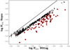 |
Fig. 3
|

3 Sample properties
In Table 3 we summarise the key properties of the sample data. Specifically, we list log (LX/Lbol) values computed from the eRASS1 X-ray flux, the median of the  values of all spectra, and those of the pseudo-simultaneous spectra. Moreover, we list the original measurements of the median of STigre of all spectra and of the pseudo-simultaneous spectra. STigre can be linearly scaled to SMWO using the conversion given in Mittag et al. (2016). Finally, we state the time difference between the middle of the eROSITA observation window and the nearest TIGRE pseudo-simultaneous observation.
We further list an observed and a computed rotation period, the derivation of which is described in Sect. 3.3. The observed period is the median value of all observational results given in the catalogues listed as footnote to Table 3. Moreover, we specify whether the star is in the valid sub-sample as defined in Sect. 2.3.1. We show the first ten rows in Table 3 for orientation, and the whole table is available electronically at CDS.
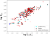 |
Fig. 4 Relation of |


3.1 Correlation between Ca II H&K and X-ray fluxes
We first compared chromospheric to coronal activity, following the ansatz of Mittag et al. (2018), using log (LX/Lbol) as the coronal activity indicator and  as a tracer of chromospheric magnetic activity. In Fig. 4 we show the
  values as a function of log (LX/Lbol) for the valid sample as defined in Sect. 2.3.1, first, using the median of all available
  values, and second, using the median of the pseudo-simultaneous values alone. For comparison, we also show the values for the Sun at solar maximum and solar minimum, respectively. The X-ray luminosity was taken from Judge et al. (2003) calculated for the ROSAT position-sensitive proportional counters (PSPC) energy band, which should be roughly comparable with our values, see Sect. 2.2. The
  values were calculated from indices taken from Schröder et al. (2017) considering the minimum or maximum value for the values they state for different cycles for solar minimum or maximum. Additionally, we mark the 48 possible binaries we found during the analysis, which mostly fall in the normal spread of the data. We inspected their properties and found that only a minority appears to be outliers, and we therefore incorporated them in our analysis for the time being. We nevertheless caution that some of the most active stars that flatten the correlation may be binaries.
Formally, log(LX/Lbol) and  are well correlated with values of 0.79 and 0.77 for Pearson’s correlation coefficient, r, if either all or only the pseudo-simultaneous data are considered, with the p-value being <10−35 in both cases. Fitting with a linear regression, we find a gradient of 0.41 in both cases, which is in line with the well-known result that the coronal X-ray flux is more sensitive to activity than the
  values.
Schrijver (1983) first noted the necessity to correct the flux in the Ca II H&K lines for the photospheric and basal contributions. When  (which contains the basal flux) is used instead of
  , the correlation deteriorates, albeit only marginally. The corresponding r-values for median
  of all data are 0.72 and also for the simultaneous data with p-values <10−30. Nevertheless, the slope of 0.3 resulting from the linear regression is lower in both cases, and we attribute this to the relatively smaller contribution of the basal activity level in the more magnetically active stars. Because the relative basal flux contribution is clearly strongest in the inactive stars, the slope of the relation is expected to flatten. We therefore confirm that
  is more closely related to coronal activity and should therefore be preferred over
  in a comparison like this.
The appearance of magnetic activity is time dependent. Both geometrical effects such as rotational modulation and changes in the magnetic field, for instance, attributable to magnetic cycles, contribute to the variation. Consequently, a better relation between individual tracers may be expected in data, which are sufficiently simultaneous to resolve these effects because the different layers of the stellar atmosphere are expected to be in a comparable state. However, no such behaviour is obvious in Fig. 4 or in the correlation coefficients stated above.
To further investigate the case, we carried out a Monte Carlo simulation to study the distribution of the correlation coefficients under the hypothesis that pseudo-simultaneity does not improve the correlation between  and log(LX/Lbol). To this end, we obtained a series of realisations of the correlation coefficient between
  and log(LX/Lbol) for our program stars, opting for one arbitrary measurement of
  for every star in the computation. Similarly, we studied the distribution of the correlation coefficient considering only pseudo-simultaneous data. In particular, we opted for one pseudo-simultaneously obtained pair of
  and log(LX/Lbol) for all stars and computed the correlation coefficient. We caution, however, that for many sample stars, only one such pair is available (and only one eRASS1 log(LX/Lbol) measurement). We executed this procedure 1000 times and show the distribution of correlation coefficients in Fig. 5 (top panel).
As obvious from Fig. 5, the distribution of correlation coefficients based on temporally uncorrelated data is far broader than that based on pseudo-simultaneous pairs, which may partly be caused by the relative sparsity of these data. The expected value derived from pseudo-simultaneous pairs is 0.76, and the probability of obtaining a similar or higher correlation coefficient from randomly associated pairs is about 20%. Consequently, we find that the correlation based on pseudo-simultaneous pairs is not significantly higher than that obtained from random associations. This is in line with the better correlation using the median of all measurements compared to pseudo-simultaneous data. This comes as a surprise because when all measurements are used, an intermediate chromospheric activity level is compared to individual coronal activity levels, which may be associated with any state of activity. Nevertheless, there is a slightly longer tail to poorer correlations in the distribution of the temporally uncorrelated data.
Because non-coordinated X-ray to optical observation pairs are often separated by more than one year, we repeated the simulations considering only TIGRE data, which are considerably “older” than the eROSITA data. This procedure obviously leads to a smaller stellar sample. For a time baseline between X-ray and optical observation of at least 200 days, a second peak at lower correlation coefficients starts to emerge. For a 750-day separation, 88 stars of the valid sample are left and a single peak at a significant lower correlation coefficient than for the pseudo-simultaneous data, as is shown in the bottom panel in Fig. 5. This shift to a lower correlation for increasingly longer time baselines starting at about 200 days suggests that cycles play a larger role in the spread of the correlation of  and log(LX/Lbol) than rotation periods do. This is in line with findings for HD 81809, for example, in which the chromospheric and coronal cycles correlate well and LX varies by nearly an order of magnitude (Orlando et al. 2017). Another example is 61 Cyg, in which the X-ray cycle is also analogue to the chromospheric cycle and X-ray brightness varies by a factor of three (Robrade et al. 2012; Robrade 2016).
Nevertheless, there may be other reasons for the large spread that is also observed in the pseudo-simultaneous data: our pseudo-simultaneous data set is hampered by the low number of data points per star. Statistical noise and possibly the effect of unresolved short-term variability caused by flares both tend to reduce correlation. Moreover, the pseudo-simultaneous window may be too long for rapidly rotating stars, which may show a different part of their surface at the optical observations. This is discussed in more detail in Sect. 3.3.
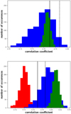 |
Fig. 5 Correlation coefficients derived by choosing |


3.2 Comparison to literature values
Mittag et al. (2018) compared  values obtained with TIGRE to non-simultaneous log(LX/Lbol) data presented by Wright et al. (2011) in a sample of 169 main-sequence stars. The logarithms of
  and log(LX/Lbol) exhibit a value of 0.76 for Spearmans’s correlation coefficient and a slope of 0.40 ± 0.02, which agrees well with the values we deduced.
Schrijver (1983) compared the X-ray surface flux and the excess flux (ΔF) in the CaII H&K lines. The latter accounts for the photospheric and basal contributions to the Ca II H&K line. They used a power-law relation  and derived ß = 1.67. If we use surface fluxes instead of luminosities (using the interpolated radius values from Pecaut & Mamajek 2013) for our data, we find ß = 1.60 with a linear regression of the logarithmic values, which agrees well with the value of Schrijver (1983).
Another study to which we can compare our results is the one by Martínez-Arnáiz et al. (2011a), who used observations of 298 F- to M-type stars for constructing various flux−flux relationships. Because the authors did not directly compare log FCa II H&K and log FX, we used the bluest component of the Ca II IRT and their log FCaII8498 to log FCa II H&K conversion from Martínez-Arnáiz et al. (2011b) additionally. Based on this, we deduce a slope of 1.58 from their studies, which is within a few percent of our number and that of Schrijver (1983) again.
3.3 Rotation and the pseudo-simultaneity
The duration of our time window for pseudo-simultaneous observations of three days before and after the start and end of the X-ray observations is largely determined by observational constraints. For stars with short rotation periods, rotational modulation can be relevant on this timescale. Evidently, a star with a rotation period of 10 days switches visible hemispheres every 5 days and rotates by a quarter in 2.5 days, where the latter already meets our criterion of pseudo-simultaneity.
To investigate the effect on our analysis, we first assessed the frequency of strong chromospheric variations on short timescales. For the 183 valid sample stars, we have a total of about 5900 TIGRE spectra, 2100 of which show a time difference of less than three days to the following spectrum. Out of these high-cadence pairs, 80 show a variation of more than 0.1 in  , which belong to 39 stars. This variation is about 100 times higher than the mean variation between spectra for the valid sample. While underestimated errors may play a role for some stars, there are many time series for which this is clearly not the case. One star (the late-F type planet host star HD 120136/τ Boo; Pro = 3.1 d by Mittag et al. (2017)) shows the largest number of detected short-term variations by far and seems to be peculiar to this respect. Out of its 780 TIGRE spectra, 25 fulfil our short-term variation criterion with many variations even occurring within a single day. The ultimate reasons for these strong variations remain unknown, but because these variations are usually relatively seldom, we argue that for most stars, they are not caused by rotation, but by flares.
To place the length of the pseudo-simultaneous observational window in the context of the rotational timescale, we need to know the stellar rotation periods. Unfortunately, directly measured rotation periods are available for only 99 sample stars, 62 of which belong to the valid sample. Fast-rotating stars tend to be more active and their periods easier to measure, and, indeed, 41 out of the 62 periods in the valid sample are shorter than 10 days; see for instance Schmitt & Mittag (2020) for the difficulties in measuring accurate periods in low-activity stars.
As an alternative to a direct measurement, rotation periods can be estimated based on the stellar activity level. Both Noyes et al. (1984) and Mittag et al. (2018) provided estimates of the rotation period, Prot, based on  . Table 3 gives the estimated rotation period based on the relation by Mittag et al. (2018) along with an observed literature period whenever available. A comparison of observed and calculated rotation period is shown in Fig. 6, where we consider both the estimates based on the Noyes et al. (1984) (red points) and Mittag et al. (2018) relations (black points). Except for some outliers, the activity-based estimates and the observed rotation periods are typically consistent to within about 3 days. The largest discrepancies occur among inactive stars, where the estimate of the basal flux also has the strongest effect on the actual
  value.
However, it is not necessarily the period estimate that is in error. Period searches are known to be sensitive also to multiples of the correct period. Cases in point may be the two stars with a measured period of about 40 d and a computed period of about 20 d (see Fig. 6), for which the latter, shorter-period estimate appears more plausible in terms of activity.
The valid sample contains 80 estimated rotation periods longer than 10 days and 103 rotation periods shorter than 10 days. As rotational modulation may therefore play a role in our consideration of pseudo-simultaneity, we divided the valid sample into slow and fast rotators with estimated rotation periods above and below 10 days, respectively.
For the fast rotators, the correlation coefficient between  and log(LX/Lbol) is 0.75 considering the median
  values and 0.76 for the pseudo-simultaneous
  values. The corresponding coefficients for the slow rotators are 0.72 and 0.70. The slopes are 0.39 for the fast and 0.43 for the slow rotators, with little dependence on whether pseudo-simultaneous or median values are considered. The pseudo-simultaneity apparently plays a smaller role than errors introduced by measurements of line indices or their conversion for inactive stars in our current data set. More pseudo-simultaneous measurements in the context of the ongoing eROSITA survey will us allow to investigate this issue in more detail.
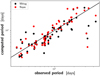 |
Fig. 6 Computed Prot vs. observed Prot for 59 stars of the valid sample with measured Prot > 2. days. |
3.4 Prediction of log(LX/Lboi) from  values
Applying a linear regression to our measured log(LX/Lbol) and  values, we obtain best-fit values for the coefficients a and b in the relation
 (1)
(1)
The values obtained for the entire valid sample as well as for spectral-type selected sub-samples are given in Table 4 and shown in Appendix A. For M dwarfs we do not have enough data points to define a meaningful fit.
The relation in Eq. (1) can be used to predict log(LX/Lbol) from, the measurement of which requires no space-based instrumentation. In Fig. 7 we show the comparison of the calculated and observed log(LX/Lbol) values as a function of  , that is, the residuals with respect to the best-fit relation. The standard deviation of the pseudo-simultaneous data in calculated minus observed (C-O) log(LX/Lbol) is 0.36 and 0.35 for the median data for the valid sample. Overall, it appears that log(LX/Lbol) is under-predicted for the most active stars, which also tend to be fast rotators. The reason for this under-prediction remains unknown. A possible physical reason would be the phenomenon of super-saturation, which is observed in X-rays (Thiemann et al. 2020, e. g.) but not in chromospheric lines (Christian et al. 2011, e. g.). However, we do not consider this very likely because the stars in our valid sample are not active enough to fall in the regime of super-saturation for X-rays, which starts for stars with v sin i > 100 km s−1. Only very few of our stars are even located at around log(LX/Lbol) = −3.14 as was observed for the saturated regime by Thiemann et al. (2020). There are two additional explanations: (i) these most active stars can be fast rotators that may cause a leaking of chromospheric flux out of the wavelength range considered for the integration for the index calculation. We are aware of two stars in the valid sample with a v sin i higher than 40 km s−1. (ii) Three of the binary candidates fall into this regime.
Inspecting the coefficients for the spectral subgroups defined in Table 4, we find that the gradients for the F and late-K type stars are lower than for the other stars. For the F-type sub-sample, this is caused by a group of stars with the lowest  values (cf. Fig. 8). There is also a slight vertical offset between the F spectral type group and the other groups for low to moderate activity levels. For the lowest activity stars, even small errors in the estimation of the basal flux (resulting, e.g. from poor fits of the PHOENIX models) lead to larger errors on the calculated
  values than is the case for more active stars, for which the magnetic contribution to the line flux is much higher than the basal flux level. Therefore we repeated the fits, omitting the most inactive stars with
  . This led to higher values for the slopes in all spectral subgroups with a significant increase observed for the F-type sub-sample. Using the spectral-type dependent relations (all valid sample stars) to predict log(LX/Lbol) leads to a slightly smaller standard deviation of 0.29 in C−O log(LX/Lbol), but log(LX/Lbol) remains under-predicted in the most active stars.
For comparison, we also used  in the linear regression because the relation by Noyes et al. (1984) remains widely used. We give here coefficients for the relation equivalent to Eq. (1) as well, which leads to a standard deviation of 0.34 for C−O log(LX/Lbol) values, comparable to the value obtained with
  .
.
 (2)
(2)
Finally, we can predict log(LX/Lbol) for the stars in our sample without eROSITA detections. By definition, these do not belong in our valid sample. All but one of them have Ca II H&K index measurements by TIGRE, and none has a B−V < 0.44 mag, which would place it outside the range of definition of our conversion relations. The calculated log(LX/Lbol) values for these stars are lower than those for the valid sample on average. While the median value of log(LX/Lbol) of the valid sample is −4.86, the predicted median of the stars without eROSITA X-ray detection is −5.99. This places most of these stars at the low-activity end of our distribution. While we cannot check the prediction at the moment, it is at least consistent with the current lack of X-ray detections.
 |
Fig. 7 Computed minus observed log(LX/Lbol) values as a function of measured Prot for stars of the valid sample with available Prot. The black dots represent the median data, and the red dots represent the pseudo-simultaneous data. |
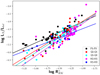 |
Fig. 8 log(LX/Lbol) values as a function of |

4 Conclusions
We investigated the chromospheric coronal connection for a sample of 404 magnetically active stars using simultaneously measured X-ray fluxes from the eRASS1 survey as tracer of the coronal activity and Ca II H&K indices derived from spectra obtained by the TIGRE telescope. From these indices, we derived  values, which we used as a proxy for the chromo-spheric activity state. The sample we presented here of (pseudo-) simultaneous coronal and chromospheric measurements is to our best knowledge the largest such sample obtained to date, comprising 183 mid-F to early-M dwarfs.
The correlation between chromospheric activity measured through  and coronal activity measured through log(LX/Lbol) somewhat surprisingly is almost identical for the median and the simultaneously measured
  values. This finding is corroborated by a bootstrap analysis, in which we randomly assigned a chromospheric measurement to the X-ray measurement. On the other hand, if only optical data “older” than two years compared to the eROSITA X-ray data are used in the bootstrap analysis, the random data pairs lead to a lower correlation than the pseudo-simultaneous data. Thus, the pseudo-simultaneous data or time series improve the correlation and are therefore desirable. In particular, the effect of activity variations on longer timescales (e.g. cycles) seems to be more important than short-term effects (e.g. rotational modulation). The effect of using median log(LX/Lbol) values can only be investigated in the future, when more eROSITA measurements with pseudo-simultaneous TIGRE data become available. We also stress that we considered only sample correlations because eROSITA time series are not yet available.
Computing the correlation between  and log(LX/Lbol) for different sub-samples in spectral type shows a tendency to higher slopes for earlier type stars. This may indicate a stronger coupling of the chromosphere and corona in earlier-type stars, but it may also be caused by an insufficient correction for the effect of spectral type by the
  conversion. Measuring the Ca II H&K index with high enough precision and correcting for the basal flux seems to be an issue for the most inactive stars where even slightly incorrect estimates of the basal flux have a relatively strong effect on the
  values and where statistical noise also has a relatively stronger effect on these weak lines. Accordingly, we find the worst correlation between
  and log(LX/Lbol) for the pseudo-simultaneous data of the slow rotators, where the opposite is expected based on timing considerations.
Predicting log(LX/Lbol) from  values is very much appealing because X-ray measurements are far more difficult to come by than ground-based determinations of the CaII H and K line flux. The predictions seem to work well for many stars with an expected standard deviation of about 0.34. We also predict mostly low log(LX/Lbol) values for the stars without an eROSITA detection. We conclude that the correlation between log(LX/Lbol) and
  is suitable to make predictions of log(LX/Lbol) from measured optical data accurate to within factors of a few. While the origin of the considerable scatter in the relation remains basically unknown, we expect contributions from (i) shortcomings in the conversion into
  values (and in the basal flux estimation) or (ii) in the non-simultaneity of the pseudo-simultaneous data for the fast rotators, and (iii) in an uncoupling of the chromospheric and coronal tracers even after subtraction of the non-magnetic heating for the chromosphere. Our results demonstrate that the ongoing eROSITA X-ray measurements in the framework of the all-sky survey along with further pseudo-simultaneous measurements by TIGRE are likely to significantly improve our understanding of the chromospheric coronal connection.
Acknowledgements
B.F. acknowledges funding by the DFG under Schm 1032/69-1. This work is based on data from eROSITA, the soft X-ray instrument aboard SRG, a joint Russian-German science mission supported by the Russian Space Agency (Roskosmos), in the interests of the Russian Academy of Sciences represented by its Space Research Institute (IKI), and the Deutsches Zentrum für Luft- und Raumfahrt (DLR). The SRG spacecraft was built by Lavochkin Association (NPOL) and its subcontractors, and is operated by NPOL with support from the Max Planck Institute for Extraterrestrial Physics (MPE). The development and construction of the eROSITA X-ray instrument was led by MPE, with contributions from the Dr. Karl Remeis Observatory Bamberg & ECAP (FAU Erlangen-Nuernberg), the University of Hamburg Observatory, the Leibniz Institute for Astrophysics Potsdam (AIP), and the Institute for Astronomy and Astrophysics of the University of Tübingen, with the support of DLR and the Max Planck Society. This work is based on data obtained with the TIGRE telescope, located at La Luz observatory, Mexico. TIGRE is a collaboration of the Hamburger Sternwarte, the Universities of Hamburg, Guanajuato and Liège. This research has made use of the SIMBAD database, operated at CDS, Strasbourg, France.
Appendix A log(Lx/Lbol) vs. R+HK per spectral type
We show the best fits for the different spectral groups together with the data in Fig. A.1. The obtained linear best fits are marked for the whole valid sample by a solid line and excluding the least active stars by a dashed line.
 |
Fig. A.1 Same as Fig. 8, but for every spectral type group separately. The solid lines mark the linear regression taking all stars into account, andthe dashed lines mark the linear regression with only the more active stars with |

References
- Armstrong, D. J., Kirk, J., Lam, K. W. F., et al. 2015, A&A, 579, A19 [NASA ADS] [CrossRef] [EDP Sciences] [Google Scholar]
- Baliunas, S., Sokoloff, D., & Soon, W. 1996, ApJ, 457, L99 [NASA ADS] [CrossRef] [Google Scholar]
- Boller, T., Freyberg, M. J., Trümper, J., et al. 2016, A&A, 588, A103 [NASA ADS] [CrossRef] [EDP Sciences] [Google Scholar]
- Brunner, H., Liu, T., Lamer, G., et al. 2022, A&A, 661, A1 (eROSITA EDR SI) [NASA ADS] [CrossRef] [EDP Sciences] [Google Scholar]
- Christian, D. J., Mathioudakis, M., Arias, T., Jardine, M., & Jess, D. B. 2011, ApJ, 738, 164 [NASA ADS] [CrossRef] [Google Scholar]
- Díaz, R. F., Cincunegui, C., & Mauas, P. J. D. 2007, MNRAS, 378, 1007 [Google Scholar]
- Fuhrmeister, B., Liefke, C., Schmitt, J. H. M. M., & Reiners, A. 2008, A&A, 487, 293 [NASA ADS] [CrossRef] [EDP Sciences] [Google Scholar]
- Fuhrmeister, B., Czesla, S., Schmitt, J. H. M. M., et al. 2019, A&A, 623, A24 [NASA ADS] [CrossRef] [EDP Sciences] [Google Scholar]
- Gaia Collaboration 2018, VizieR Online Data Catalog: I/345 [Google Scholar]
- Gomes da Silva, J., Santos, N. C., Bonfils, X., et al. 2011, A&A, 534, A30 [NASA ADS] [CrossRef] [EDP Sciences] [Google Scholar]
- Güdel, M. 2004, A&ARv, 12, 71 [CrossRef] [Google Scholar]
- Hartmann, L., Soderblom, D. R., Noyes, R. W., Burnham, N., & Vaughan, A. H. 1984, ApJ, 276, 254 [Google Scholar]
- Hauschildt, P. H., Allard, F., & Baron, E. 1999, ApJ, 512, 377 [Google Scholar]
- He, L., Wang, S., Liu, J., et al. 2019, ApJ, 871, 193 [NASA ADS] [CrossRef] [Google Scholar]
- Hempelmann, A., Robrade, J., Schmitt, J. H. M. M., et al. 2006, A&A, 460, 261 [NASA ADS] [CrossRef] [EDP Sciences] [Google Scholar]
- Judge, P. G., Solomon, S. C., & Ayres, T. R. 2003, ApJ, 593, 534 [NASA ADS] [CrossRef] [Google Scholar]
- Kiraga, M. 2012, Acta Astron., 62, 67 [NASA ADS] [Google Scholar]
- Martínez-Arnáiz, R., López-Santiago, J., Crespo-Chacón, I., & Montes, D. 2011a, MNRAS, 414, 2629 [CrossRef] [Google Scholar]
- Martínez-Arnáiz, R., López-Santiago, J., Crespo-Chacón, I., & Montes, D. 2011b, MNRAS, 417, 3100 [CrossRef] [Google Scholar]
- Mathioudakis, M., & Doyle, J. G. 1992, A&A, 262, 523 [NASA ADS] [Google Scholar]
- Mittag, M., Schmitt, J. H. M. M., & Schröder, K. P. 2013, A&A, 549, A117 [NASA ADS] [CrossRef] [EDP Sciences] [Google Scholar]
- Mittag, M., Schroder, K. P., Hempelmann, A., González-Pérez, J. N., & Schmitt, J. H. M. M. 2016, A&A, 591, A89 [NASA ADS] [CrossRef] [EDP Sciences] [Google Scholar]
- Mittag, M., Robrade, J., Schmitt, J. H. M. M., et al. 2017, A&A, 600, A119 [NASA ADS] [CrossRef] [EDP Sciences] [Google Scholar]
- Mittag, M., Schmitt, J. H. M. M., & Schröder, K. P. 2018, A&A, 618, A48 [NASA ADS] [CrossRef] [EDP Sciences] [Google Scholar]
- Noyes, R. W., Hartmann, L. W., Baliunas, S. L., Duncan, D. K., & Vaughan, A. H. 1984, ApJ, 279, 763 [Google Scholar]
- Orlando, S., Favata, F., Micela, G., et al. 2017, A&A, 605, A19 [NASA ADS] [CrossRef] [EDP Sciences] [Google Scholar]
- Pecaut, M. J., & Mamajek, E. E. 2013, ApJS, 208, 9 [Google Scholar]
- Predehl, P., Andritschke, R., Arefiev, V., et al. 2021, A&A, 647, A1 [EDP Sciences] [Google Scholar]
- Reinhold, T., & Hekker, S. 2020, A&A, 635, A43 [NASA ADS] [CrossRef] [EDP Sciences] [Google Scholar]
- Robertson, P., Bender, C., Mahadevan, S., Roy, A., & Ramsey, L. W. 2016, ApJ, 832, 112 [CrossRef] [Google Scholar]
- Robrade, J. 2016, in XMM-Newton: the Next Decade, ed. J.-U. Ness, 112 [Google Scholar]
- Robrade, J., & Schmitt, J. H. M. M. 2005, A&A, 435, 1073 [NASA ADS] [CrossRef] [EDP Sciences] [Google Scholar]
- Robrade, J., Schmitt, J. H. M. M., & Favata, F. 2012, A&A, 543, A84 [NASA ADS] [CrossRef] [EDP Sciences] [Google Scholar]
- Rutten, R. G. M., Schrijver, C. J., Lemmens, A. F. P., & Zwaan, C. 1991, A&A, 252, 203 [NASA ADS] [Google Scholar]
- Samus’, N. N., Kazarovets, E. V., Durlevich, O. V., Kireeva, N. N., & Pastukhova, E. N. 2017, Astron. Rep., 61, 80 [Google Scholar]
- Schmitt, J. H. M. M. 1997, A&A, 318, 215 [NASA ADS] [Google Scholar]
- Schmitt, J. H. M. M., Fleming, T. A., & Giampapa, M. S. 1995, ApJ, 450, 392 [Google Scholar]
- Schmitt, J. H. M. M., Schroder, K. P., Rauw, G., et al. 2014, Astron. Nachr., 335, 787 [NASA ADS] [CrossRef] [Google Scholar]
- Schmitt, J. H. M. M., & Mittag, M. 2020, Astron. Nachr., 341, 497 [NASA ADS] [CrossRef] [Google Scholar]
- Schöfer, P., Jeffers, S. V., Reiners, A., et al. 2019, A&A, 623, A44 [Google Scholar]
- Schrijver, C. J. 1983, A&A, 127, 289 [NASA ADS] [Google Scholar]
- Schrijver, C. J. 1987, A&A, 172, 111 [NASA ADS] [Google Scholar]
- Schrijver, C. J. 1995, A&ARv, 6, 181 [NASA ADS] [CrossRef] [Google Scholar]
- Schrijver, C. J., Dobson, A. K., & Radick, R. R. 1992, A&A, 258, 432 [NASA ADS] [Google Scholar]
- Schröder, K. P., Mittag, M., Schmitt, J. H. M. M., et al. 2017, MNRAS, 470, 276 [CrossRef] [Google Scholar]
- Stepien, K., & Ulmschneider, P. 1989, A&A, 216, 139 [NASA ADS] [Google Scholar]
- Suárez Mascareño, A., Rebolo, R., & Gonzalez Hernandez J.I. 2016, A&A, 595, A12 [NASA ADS] [CrossRef] [EDP Sciences] [Google Scholar]
- Thiemann, H. B., Norton, A. J., & Kolb, U. C. 2020, PASA, 37, e042 [NASA ADS] [CrossRef] [Google Scholar]
- van Leeuwen, F. 2007, A&A, 474, 653 Walkowicz, L. M., & Hawley, S. L. 2009, AJ, 137, 3297 [Google Scholar]
- Wedemeyer, S., Freytag, B., Steffen, M., Ludwig, H. G., & Holweger, H. 2004, A&A, 414, 1121 [NASA ADS] [CrossRef] [EDP Sciences] [Google Scholar]
- Wenger, M., Ochsenbein, F., Egret, D., et al. 2000, A&AS, 143, 9 [NASA ADS] [CrossRef] [EDP Sciences] [Google Scholar]
- Wilson, O. C. 1978, ApJ, 226, 379 [Google Scholar]
- Wright, J. T., Marcy, G. W., Butler, R. P., & Vogt, S. S. 2004, ApJS, 152, 261 [Google Scholar]
- Wright, N. J., Drake, J. J., Mamajek, E. E., & Henry, G. W. 2011, ApJ, 743, 48 [Google Scholar]
We adopted B−V values from SIMBAD (Wenger et al. 2000) for all stars but HD 97503, where the HIPPARCOS main catalogue was used (van Leeuwen 2007).
All Tables
All Figures
|
Fig. 1 HR diagram of a sub-sample of our stars defined as a valid sample in Sect. 2.3.1 that also shows the X-ray properties of these stars. |
| In the text | |
|
Fig. 2 Number of spectra taken by TIGRE for a certain offset between the middle of the eROSITA observation and the time of the TIGRE observations for pseudo-simultaneous data. |
| In the text | |
|
Fig. 3
|
| In the text | |
|
Fig. 4 Relation of |
| In the text | |
|
Fig. 5 Correlation coefficients derived by choosing |
| In the text | |
|
Fig. 6 Computed Prot vs. observed Prot for 59 stars of the valid sample with measured Prot > 2. days. |
| In the text | |
|
Fig. 7 Computed minus observed log(LX/Lbol) values as a function of measured Prot for stars of the valid sample with available Prot. The black dots represent the median data, and the red dots represent the pseudo-simultaneous data. |
| In the text | |
|
Fig. 8 log(LX/Lbol) values as a function of |
| In the text | |
|
Fig. A.1 Same as Fig. 8, but for every spectral type group separately. The solid lines mark the linear regression taking all stars into account, andthe dashed lines mark the linear regression with only the more active stars with |
| In the text | |
Current usage metrics show cumulative count of Article Views (full-text article views including HTML views, PDF and ePub downloads, according to the available data) and Abstracts Views on Vision4Press platform.
Data correspond to usage on the plateform after 2015. The current usage metrics is available 48-96 hours after online publication and is updated daily on week days.
Initial download of the metrics may take a while.