| Issue |
A&A
Volume 660, April 2022
|
|
|---|---|---|
| Article Number | A54 | |
| Number of page(s) | 9 | |
| Section | The Sun and the Heliosphere | |
| DOI | https://doi.org/10.1051/0004-6361/202142907 | |
| Published online | 12 April 2022 | |
Extension and validation of the pendulum model for longitudinal solar prominence oscillations
1
Departament Física, Universitat de les Illes Balears, 07122 Palma de Mallorca, Spain
e-mail: This email address is being protected from spambots. You need JavaScript enabled to view it.
2
Institute of Applied Computing & Community Code (IAC 3), UIB, Spain
3
Heliophysics Science Division, NASA Goddard Space Flight Center, 8800 Greenbelt Road, Greenbelt, MD 20771, USA
Received:
14
December
2021
Accepted:
10
February
2022
Abstract
Context. Longitudinal oscillations in prominences are common phenomena on the Sun. These oscillations can be used to infer the geometry and intensity of the filament magnetic field. Previous theoretical studies of longitudinal oscillations made two simplifying assumptions: uniform gravity and semicircular dips on the supporting flux tubes. However, the gravity is not uniform and realistic dips are not semicircular.
Aims. Our aim is to understand the effects of including the nonuniform solar gravity on longitudinal oscillations and explore the validity of the pendulum model with different flux-tube geometries.
Methods. We first derived the equation describing the motion of the plasma along the flux tube including the effects of nonuniform gravity, yielding corrections to the original pendulum model. We also computed the full numerical solutions for the normal modes and compared them with the new pendulum approximation.
Results. We find that the nonuniform gravity introduces a significant modification in the pendulum model. We also found a cut-off period; i.e., the longitudinal oscillations cannot have a period longer than 167 min. In addition, considering different tube geometries, the period depends almost exclusively on the radius of curvature at the bottom of the dip.
Conclusions. We conclude that nonuniform gravity significantly modifies the pendulum model. These corrections are important for prominence seismology, because the inferred values of the radius of curvature and minimum magnetic-field strength differ substantially from those of the old model. However, we find that the corrected pendulum model is quite robust and is still valid for noncircular dips.
Key words: Sun: corona / Sun: filaments / prominences / Sun: magnetic fields / Sun: oscillations
© ESO 2022
1. Introduction
Solar prominences are very dynamical objects with many kinds of motions, including oscillations and wave phenomena. A common type of motion is large-amplitude oscillations, in which a large portion of the filament oscillates coherently with velocities above 10 km s−1. These oscillations have been reported since the first half of the twentieth century (see the review of Arregui et al. 2018). Jing et al. (2003) identified large-amplitude longitudinal oscillations (LALOs) along prominence threads after a nearby energetic event, and many more LALOs have been reported since then (see Luna et al. 2018). LALOs are excited by eruptive flares near the filament (e.g., Jing et al. 2003; Vršnak et al. 2007; Zhang et al. 2012), jets (Luna et al. 2014; Zhang et al. 2017), or coronal shocks (Shen et al. 2014). However, in many cases the trigger agent has not been identified. LALO periods range from a few tens of minutes up to 160 min (Jing et al. 2006), but most of the reported events have periods of around one hour (Luna et al. 2018).
Large-amplitude longitudinal oscillations are important because they can be used to infer the geometry and intensity of the filament magnetic field (Luna & Karpen 2012; Zhang et al. 2012; Luna et al. 2014, 2017). Prominence magnetic structure is a long-standing question, because we can only observe the photospheric field directly, and competing models have been proposed. Because prominences reside in filament channels, which are the sources of all major solar eruptions, understanding the full coronal structure of these channels is crucial for resolving the fundamental physical mechanism(s) responsible for eruptions and resulting space weather. One key consequence of the LALO phenomenon is that the flux tubes supporting and guiding the prominence plasma must contain dips: concave upward regions in which Lorentz forces balance the gravitational force. This constraint led to a surprisingly accurate “pendulum” model for LALO motions, and a new prominence-seismology technique for deriving the dip radius of curvature and the minimum magnetic-field strength in the dip (Luna & Karpen 2012; Luna et al. 2014).
Previous theoretical studies of longitudinal oscillations made two simplifying assumptions that we explore further in this paper: uniform gravity and semicircular dips on the supporting flux tubes. The first assumption is to consider gravity as a uniform vector with a value of 274 m s−2, which is vertical at all points of the studied volume. This approximation is widely used in theoretical studies when the region studied is a small portion of the Sun. Examples of theoretical studies of longitudinal oscillations using uniform gravity include Luna & Karpen (2012), Zhang et al. (2013), Luna et al. (2016b), Terradas et al. (2016), and Liakh et al. (2020). However, gravity is not uniform and depends on position. The gravity vector always points to the center of the Sun, and its intensity decreases with distance. As we demonstrate in this paper, the spatial dependence of gravity can strongly influence longitudinal oscillations of solar prominences. Secondly, previous models assumed semicircular dips of the field lines supporting the prominence threads (Luna & Karpen 2012; Luna et al. 2012, 2016a). In this geometry, the radius of curvature along the dip, R0, is constant. However, in a realistic situation, the curvature is not likely to be constant. The radius of curvature depends on the position along the dip R = R(s) with R0 = R(s = 0), where s is the coordinate along the flux tube and s = 0 at the bottom of the dip. In this situation, the relation between the period and the radius of curvature is not immediately obvious. Numerical simulations of longitudinal oscillations in different flux-tube geometries (see, e.g., Zhang et al. 2013; Luna et al. 2016b; Liakh et al. 2021) have shown that the pendulum model is still valid considering the radius of curvature at the bottom of the dip, R0, or a curvature averaged around the center of the dip. In the present study, we investigate the robustness of the model and identify under which conditions the pendulum model remains valid.
In this study, we consider that LALOs can be described by linear magnetoacoustic-gravitational modes (Luna et al. 2012; Terradas et al. 2013). This allows us to study LALOs analytically and find useful relationships that apply to prominence seismology. However, the displacements and velocities in LALOs are large and nonlinear effects may be relevant. Nonlinear effects will be considered in a future study. In this paper, we present the effects of including the nonuniform solar gravity and then explore the validity of the pendulum model with different flux-tube geometries. In Sect. 2, we introduce the model that describes the equilibrium and dynamics of a prominence thread with the nonuniform gravity incorporated. In Sect. 3, the longitudinal oscillations in a flux tube with semicircular dip geometry are studied to find the influence of curvature of the solar surface. In Sect. 4, the study is extended to alternative flux-tube geometries to investigate the validity of the pendulum model in these geometries. In Sect. 5, we discuss the influence of the solar-surface curvature on the determination of the radius of curvature of the dips and the minimum magnetic-field strength of the prominences using seismology. Finally, in Sect. 6, the conclusions of this investigation are summarised.
2. The model
Here, we derive the equation that describes the motion of the plasma velocity perturbations including the intrinsic spatial variations of the solar gravity. We also show the different flux-tube geometries used to determine the influence of the dip shape on the oscillations. Finally we consider the equilibrium of the plasma along the flux tube. We assume that the central part is filled with cool prominence plasma representing a thread. The temperature increases sharply at its sides, reaching a coronal temperature that applies to the rest of the tube up to the footpoints.
2.1. Nonuniform gravity considerations
The solar gravity is given by the expression
 (1)
(1)
where g0 = 274 m s−2 is the acceleration at the solar surface, h is the height with respect to the solar surface, and  is the radial unit vector pointing in the (minus) direction of gravity. Most prominences are located in the low corona, in which h ≪ R⊙. Thus, Eq. (1) can be approximated by
 (2)
(2)
This indicates that, for filaments in the low corona, the main spatial variation of gravity is due to its changing direction, not its intensity. The novelty of this work is to introduce this intrinsic variation of the solar gravity with position. For the study of longitudinal oscillations, we are interested in the projection of the gravity along the magnetic field of solar prominences, g∥. It is important to note that, in the uniform gravity situation, g∥ changes along the field line because the magnetic-field direction changes. However, in the nonuniform situation, g∥ also changes with the intrinsic changes of the direction of g given by Eq. (2).
2.2. The governing equation
The oscillations along the magnetic field in 2D configurations were described by Goossens et al. (1985) as so-called slow continuum modes, also denoted magnetoacoustic-gravity modes (Terradas et al. 2013). In contrast to usual MHD slow modes, both gas-pressure gradients and gravity can be the restoring forces of these modes. We assumed a low-β, adiabatic plasma confined in uniform cross-section flux tubes along a static magnetic field with with no heating or radiation terms, similarly to Luna et al. (2012, hereafter Paper I). The novelty is that we considered the intrinsic spatial variations of the solar gravity field using Eq. (2). With these assumptions, from the ideal MHD equations, we recover our previous expression (Eq. (5) in Paper I):
 (3)
(3)
where  is the sound speed and p and ρ are the equilibrium gas pressure and density, respectively. We note that g∥ depends on the position s due to two contributions: the change in the projection of the gravity along the field line and the intrinsic variation of the gravity field (Eq. (2)) that is introduced in this work. Assuming a harmonic time dependence, eiωt, the governing equation becomes
 (4)
(4)
Both terms g∥ and ∂g∥/∂s depend on the geometry of the flux tube. For a semicircular dip, it is still possible to gain some insight into the effect of the intrinsic spatial variation of gravity (see Sect. 3) using an analytical approach. However, it is difficult to find an analytic expression for both terms for more general geometries, so we solved Eq. (4) numerically for different shapes of the flux tubes.
2.3. Flux tube models
In this work, we explored the possible dependence of longitudinal oscillations on the geometry of the field lines. Although there are many possibilities, we considered three geometries for the flux tubes shown in Fig. 1. We chose these cases because they are described by functions of a few parameters that allow us to control the shape of the flux tube. The first one (Model 1, Fig. 1a) consists of a central, semicircular segment of radius R. On both sides, there is a straight part representing the nondipped part of the tube. The semicircular dip and the straight parts are joined smoothly with a small arc with Rsmall = 10 Mm, which is tangent to the central and the straight parts. We considered a range of R from 42 to 1000 Mm. The lengths of the different parts of the piecewise flux tube were changed to keep the total half-length of the tube to L1/2 = 100 Mm.
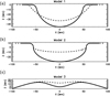 |
Fig. 1. Flux tube geometries considered in this work: (a) semicircular dip, (b) elliptical dip, and (c) sinusoidal dip. The solid line is the flux tube with the smallest radius of curvature. The dashed line is a case with a radius of curvature intermediate between the minimum and the maximum. In both Models 1 and 2, the end points of the flux-tube components change in order to keep the total length of the field line constant. |
Model 2 consists of a central, semi-elliptical segment with major axis a = 55 Mm parallel to x (Fig. 1b); minor axis, b, is parallel to z and ranges from b = 3 to 55. The tube also has two straight, horizontal segments as in Model 1. The dipped and straight parts are joined smoothly with an arc of Rsmall = 8 Mm. The length of the straight part is varied to keep the half-length of the tube to L1/2 = 100 Mm. The radius of curvature of the dipped part depends on the parameter b. At the bottom of the dip (i.e., the central position), the radius of curvature is
 (5)
(5)
With the parameters stated above for Model 2, R0 ranges from 37 to 1000 Mm.
Model 3 is the most realistic because the footpoints are anchored in the solar surface. The flux tube consists of a combination of sinusoidal functions:
![Mathematical equation: $$ \begin{aligned} z(x)=A_0 \cos \left(\frac{2 \pi x}{\lambda _0}\right)-A_1 \left[\cos \left(\frac{2 \pi x}{\lambda _1}\right)+1\right]^n , \end{aligned} $$](/articles/aa/full_html/2022/04/aa42907-21/aa42907-21-eq8.gif) (6)
(6)
where λ0 = 399 Mm, λ1 = λ0/2, n = 4, A0 = 20 Mm and A1 = 0.18 − 1 Mm. The z-position of the dip changes with A1 as zdip = A0 − A1 2n and ranges from 4 to 17 Mm. With the selected parameters, the half-length of the tube is more or less constant: L1/2 = 100 Mm. The radius of curvature at the bottom of the dip is given by
 (7)
(7)
With the parameters considered in this work, Model 3 has R0 = 55 − 1000 Mm.
The plasma equilibrium is stratified following the equation
 (8)
(8)
The projected gravity, g∥, is given by Eq. (2), where the effect of the change of direction is incorporated. However, we note that the governing Eq. (4) only depends on the sound speed cs, which is proportional to the square root of the temperature. To solve Eq. (4), we calculate cs from the following temperature profile:
![Mathematical equation: $$ \begin{aligned} {T(s)= {\left\{ \begin{array}{ll} T_\mathrm{p} ,&\mathrm{if}\ |s| \le -l_{1/2} \\ T_{+} +T_{-} \cos \left[ \frac{\pi }{l_\mathrm{tr} } (|s|-l_{1/2}) \right] ,&\mathrm{if}\ l_{1/2} < |s|\le l_{1/2}+l_\mathrm{tr} \\ T_\mathrm{c} ,&\mathrm{if}\ |s|\le l_{1/2}+l_\mathrm{tr} \end{array}\right.} } ,\end{aligned} $$](/articles/aa/full_html/2022/04/aa42907-21/aa42907-21-eq11.gif) (9)
(9)
where Tp = 6 × 10³K, Tc = 106K, T+ = (Tc+Tp)/2, and T− = (Tc−Tp)/2. Tp and Tc are the prominence and corona equilibrium temperatures, respectively. The assumed half-length of the prominence thread is l1/2 = 5 Mm, and the temperature changes smoothly from prominence to coronal temperatures within a distance ltr = 1 Mm at both ends of the thread. We tested different sizes for ltr, and its influence on the results is small.
3. Semicircular geometry
The semicircular dip geometry is the simplest, and has been used in previous LALO research (e.g., Luna et al. 2012; Ruderman & Luna 2016). Now we show how the intrinsic variations of the solar gravity in this geometry introduce corrections in the longitudinal oscillations.
3.1. Pendulum approximation
Figure 2 shows the very simplified situation of a semicircular dip of radius R (thick solid curve). The center of curvature of the dip segment is C.
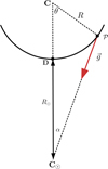 |
Fig. 2. Sketch of a dip with circular shape (solid line) with radius R. The red arrow shows the solar gravity on a point of the tube (𝒫) pointing to the center of the Sun, C⊙. |
Many prominences are located in the low corona, so their heights above the surface, h, are small relative to R⊙. The distance from the Sun’s center, C⊙ to the bottom of the dip, D, is d(C⊙,D) = R⊙ + h. However, h/R⊙ ≪ 1 so d(C⊙,D) ≈ R⊙. This is equivalent to considering that the lower part of the dip is in contact with the surface as shown in the sketch (Fig. 2). The gravity always points to the solar center, C⊙. The relation between the angles θ and α is
 (10)
(10)
Any fluid element with position 𝒫 moves along the semicircular dip. We expect that the distance of any fluid element from the central position is small in comparison with the solar radius. Thus, R sin θ ≪ R⊙. Therefore, Eq. (10) can be approximated as
 (11)
(11)
The gravity vector is g = −g0 (sin α, cos α), and the tangent unitary vector along the field line is u = (cos θ, sin θ). The scalar product of both vectors gives the projection of the gravity along the field line:
 (12)
(12)
With Eq. (11), we obtain an approximated expression for the projected gravity
 (13)
(13)
where we used the identity θ = s/R. This equation shows the dependence of g∥ on position s. On the right side, there are two contributions. The first is associated with the change of magnetic-field direction along the line and therefore the change of projection of gravity. The second is associated with the intrinsic variation of nonuniform gravity. In an ideal situation with a straight horizontal tube, R = ∞, the projection of gravity is not zero. This contrasts with the uniform gravity case, R⊙ = ∞, where the projection is zero. Introducing Eq. (13) into (4) yields
![Mathematical equation: $$ \begin{aligned} c_{s}^{2} \frac{\partial ^{2} { v}}{\partial s^{2}} -\gamma {{g_0}}s \left(\frac{1}{R}+\frac{1}{R_\odot } \right)\frac{\partial { v}}{\partial s} + { v} \left[\omega ^{2}-{{g_0}}\, \left(\frac{1}{R}+\frac{1}{R_\odot }\right) \right] =0. \end{aligned} $$](/articles/aa/full_html/2022/04/aa42907-21/aa42907-21-eq16.gif) (14)
(14)
In this modified equation of motion, the curvature of the flux-tube dip and the curvature of the solar surface are included, in contrast to Eq. (7) of Paper I. We define an equivalent radius of curvature as
 (15)
(15)
Substituting Eq. (15) for Eq. (4), we obtain a formally equivalent expression to Eq. (9) from Paper I. Taking advantage of this, we find that the oscillation frequency in a semicircular dip is described by the equivalent to Eq. (25) in Paper I, but now with Req instead of R, namely
 (16)
(16)
where the first two terms are associated with the gravity and the last ωslow is the slow-mode angular frequency associated with the gas-pressure gradient. In Sect. 3.2, we present an approximation for this frequency. In prominences, the slow-mode term is negligible compared to the terms associated with the solar gravity remaining in the pendulum model (see Paper I). The period is given by
 (17)
(17)
We define the period with uniform gravity as  . Then,
 (18)
(18)
Hence, the period is not affected by the solar curvature, P ≈ P0, when R ≪ R⊙. Figure 3 shows a plot of both periods, P and P0, as functions of the period of the uniform-gravity case, P0. For R ≪ R⊙, both periods are almost identical, as expected. However, for increasing values of P0 the P curve starts to diverge from the diagonal, becoming particularly evident beyond 50 min. This figure shows that the solar-surface curvature introduces a very small corrections for typical LALO periods of around one hour, but the deviation is significant for longer periods.
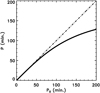 |
Fig. 3. Corrected pendulum period Eq. (18) as a function of the old pendulum period P0 (solid line). The dot-dashed line is plotted to show the diagonal where P = P0. We see that the period deviates from the diagonal for periods larger than 50 min. |
3.2. The existence of a maximum pendulum period
Prominence threads are supported against gravity by the magnetic field. At the bottom of the dips, the Lorentz force points in the vertical direction (i.e.,  in Cartesian coordinates) such that
 (19)
(19)
where the first term on the right side is the magnetic pressure gradient and the second term is the magnetic tension (see Priest 2014). Although the dips are not necessarily semicircular and the radius of curvature depends on the position, R is the curvature at the bottom of the dip in Eq. (19). The tension term points upward, whereas the magnetic pressure gradient points downward. This implies that  , i.e., the field strength increases with z as observed in the prominence core where the cool plasma is located (e.g., Rust 1967; Leroy et al. 1983). If the field is approximately force-free, these two terms are nearly balanced. With the presence of the prominence mass, a small excess of magnetic tension provides support against gravity. This additional magnetic tension is given by a perturbation of the magnetic configuration with respect to the force-free configuration.
Equation (19) shows that the support against gravity is given by the curvature of the dipped part of the flux tubes. The only possibility to have support is for positive values of the radius of curvature, R > 0. For negative values of R, the magnetic configuration is a loop. In this sense, to have a prominence supported against gravity, R ∈ (0, ∞), where R = ∞ corresponds to a straight line. By substituting progressively increasing values of R into Eq. (17), we see that the term 1/R tends to zero, and the period, P, tends asymptotically to  and never exceeds this value, because when R approaches infinity there is no dip and therefore no possibility of support against gravity. The cut-off frequency corresponds to a period of
 (20)
(20)
Figure 4 shows the period as a function of the radius of curvature of the dip using the pendulum approximation (17). For large values of R, the period curve approaches P⊙, whereas P0 increases monotonically with R.
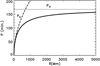 |
Fig. 4. Corrected period (Eq. (17)) as a function of R (solid line). For comparison, the dashed line shows the uncorrected pendulum period P0. The horizontal dotted line shows the cut-off period P⊙, toward which P tends asymptotically. |
3.3. Effect of gas pressure
The previous analysis is valid when the pendulum approximation is applicable. However, in general, the contribution of the gas pressure should be considered. To find the normal modes of flux tube Model 1 (Fig. 1a), we solve Eq. (4) numerically. Line-tying conditions are imposed at the footpoints, and the eigenvalue problem is solved by means of a shooting technique. The numerical routine provides the eigenfunction and the corresponding eigenfrequency of the different modes allowed in the system (see further details in Terradas et al. 2013). Figure 5 shows the periods of the fundamental normal mode computed numerically, the corrected pendulum period from Eq. (17) and the original (uncorrected) pendulum period P0.
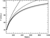 |
Fig. 5. Period of fundamental-mode period found by solving Eq. (4) for Model 1 (solid line). The dotted line is the approximation given by Eq. (21), the dashed line shows the corrected pendulum period from Eq. (17), and the dot-dashed line is the uncorrected pendulum-model period P0. |
All periods shown in the figure are similar with regard to small R and increase with radius of curvature. For relatively large R values, however, the period P differs considerably from the corrected pendulum approximation because P is significantly modified by the slow-mode contribution in this model flux tube. We also plotted the period given by the approximation from Eq. (16). From this equation, the period is
 (21)
(21)
The period Pslow = 2π/ωslow is computed numerically by solving Eq. (14) assuming g0 = 0 and finding the normal mode. In this configuration, the slow-mode period is independent of the field-line geometry and equal to Pslow = 206 min. We derive an approximate expression for Pslow by modifying Eq. (26) from Paper I, namely
 (22)
(22)
where χ = Tc/Tp is the temperature ratio between the coronal plasma and the prominence. csc is the sound speed at the corona with temperature Tc. In Paper I the parameter  equals the half-length of the prominence l1/2 because there is a sharp transition between prominence and corona. Here, in contrast, we have a smooth transition between both media given by Eq. (9). Using
  approximates the exact value of Pslowvery well.
The period P containing all contributions agrees very well with the exact numerical solution (dotted line in Fig. 5). From Eq. (21), we find that the period approaches the following cut-off value as R → ∞:
 (23)
(23)
For small values of Pslow, Pcutoff ≈ Pslow. In contrast, for Pslow ≫ P⊙, Pcutoff → P⊙, and P < Pcutoff < P⊙. In this configuration, Pslow = 206 min computed numerically, and thus Pcutoff = 130 min. Equation (21) shows that the longitudinal oscillation period cannot be larger than P⊙. It is interesting that Jing et al. (2006) found an event with a period of 160 min, which is close to P⊙. Therefore, Pslow should be much larger than the cut-off period in that event. Prominence oscillations with very long (5–6 h) and ultra-long (up to 30 h) periods have been reported (Foullon et al. 2004, 2009; Pouget et al. 2006). The existence of Pcutoff implies that these very low frequency oscillations cannot be attributed to the fundamental magnetoacoustic-gravity mode.
Longitudinal oscillations are governed by two possible restoring forces: the projected gravity and the gas-pressure gradients. In Paper I, we found that the gravity dominates when R ≪ Rlim in a situation of uniform gravity, where  depends on different parameters of the flux tube and the thread. For the case of nonuniform gravity, the relation becomes Req ≪ Rlim. Using Eq. (15), we obtain a new condition on the radius of curvature of the field lines as
  where
where
 (24)
(24)
This is easier to fulfil than the equivalent condition for uniform gravity. With the parameter values stated above, Rlim ≈ 1100 Mm, and the new maximum radius is  .
.
Figure 6a shows the eigenfunctions, v = v(s), obtained by solving Eq. (4) numerically. We find a clear dependence on the curvature radius. For the most curved (smallest R) dip in Model 1, the velocity has a wide plateau around the center, extending across the entire dip. In contrast, for an almost flat flux tube, the velocity is mainly concentrated in the dense thread region at the bottom of the dip and the shape of the eigenfunction is almost triangular. Ranging from small to large values of R, the eigenfunction continuously changes from a plateau to a triangular shape. We considered the same case without the effect of the solar surface curvature, i.e., R⊙ = ∞. Figure 6a shows the velocity profile for the normal modes of both maximum and minimum values of R0 with uniform gravity. The case with the minimum R0 is very similar to the thick solid line. Similarly, the case with the maximum R0 is almost identical to the thick gray line. This indicates that there are no important differences between the eigenfunctions in both situations. Therefore, although the effect of the solar curvature modifies the oscillation period, it does not significantly affect the velocity profile of the fundamental normal mode.
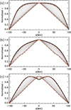 |
Fig. 6. Eigenfunction v = v(s) solutions of Eq. (4) normalised to its maximum value for (a) circular, (b) elliptical, and (c) sinusoidal tube models (see Fig. 1). The thick black line corresponds to the mode with the minimum radius of curvature for each model (see Sect. 2.3), and the thick gray line corresponds to R0 = 1000 Mm. The thin lines correspond to eigenfunctions with intermediate R0 values, smoothly transitioning between both extreme functions. The two red dashed lines in (a) are the normal modes for both maxima and minima of R0 for the uniform-gravity case. |
4. Alternative geometries
We computed the oscillations of the fundamental mode in Models 2 and 3, in which the central segment assumes semielliptical and sinusoidal shapes, respectively. We compared the period predicted by the pendulum model with the period corresponding to the radius of curvature at the center of the dip, R0, given by Eqs. (5) and (7) for these models.
Figure 7a shows the period as a function of the radius of curvature at the bottom of the dip for the three models considered in this work. The periods of the semicircular and semielliptical dip geometries are very similar. Model 2 has periods slightly smaller than the semicircular case, while the Model 3 periods are larger than for Model 1. In both cases, the discrepancies are very small for small radii of curvature and increase with R0. This figure shows that the periods are roughly independent of the flux-tube geometry for periods below 120 min.
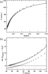 |
Fig. 7. Comparison of (a) period as a function of curvature radius at the bottom of the dip, R0, for the three geometries considered: Model 1 (solid line), Model 2 (circles), and Model 3 (diamonds). In (b) the comparison of the percentage of discrepancy between the exact period and that estimated by the corrected pendulum model (Eq. (17)) as a function of the exact period. |
Figure 7b shows the difference between the actual fundamental-mode period, P, and the corrected pendulum-model period Ppendulum given by Eq. (17), as a function of the period P. This difference is expressed in % as 100(Ppendulum − P)/P. The discrepancy with the pendulum model is below 5% for periods of less than 75 min, and it increases with P. For Models 1 and 2, the discrepancies are below 10% for periods under 95 min. In contrast, for the sinusoidal geometry (Model 3), the difference is below 10% in all of the displayed domain. The differences between the curves are not very significant, which leads us to conclude that the range of validity of the pendulum model is similar for all geometries.
The eigenfunctions v = v(s) for Models 2 and 3 are shown in Figs. 6b,c. The functions for the semi-elliptical case are similar to those of the semicircular geometry (Fig. 6a), with the maximum velocity located at the tube center. For small R the function is very flat, but there is no clear plateau as in Model 1. For flatter tubes with larger eccentricity, the motion is more and more confined in the cool thread; the eigenfunction shape becomes more triangular as the eccentricity increases. The function has a small deviation at around |s| = 55 Mm that is an artifact of the transition between the dip and the adjoining straight horizontal tubes. The Model 3 eigenfunctions differ substantially from those of the other models. For deep dips, the eigenfunction has two maxima not located at the dip bottom. For shallower dips, the function changes and the two maxima approach one another as R decreases. Finally, for the flattest tubes, the function resembles a triangle, as in previous models. As for Model 1, we also computed the eigenfunctions in the case of uniform gravity and found negligible differences with the nonuniform gravity case (see red dashed lines).
5. Influence on prominence seismology
The prominence-seismology technique combines theoretical modeling of prominence oscillations with observations to infer hidden or hard-to-measure features of the prominence structure. LALOs provide unique measurements of the curvature of the dips in filament-channel flux tubes, and a minimum value for the magnetic-field strength in those dips (e.g., Luna & Karpen 2012). The relations between the oscillation period and these two parameters have changed from our earlier results, due to the corrections introduced by the intrinsic spatial variation of the solar gravity. Assuming that the pendulum model works well (i.e., Pslow → ∞), Eq. (21) yields a new relation between the radius of curvature and the period:
![Mathematical equation: $$ \begin{aligned} R=\frac{{{g_0}}\, P^2 }{4\pi ^2\left[1-\left(\frac{P}{P_\odot }\right)^2\right]}=\frac{R_\mathrm{old} }{1-\left(\frac{P}{P_\odot }\right)^2} , \end{aligned} $$](/articles/aa/full_html/2022/04/aa42907-21/aa42907-21-eq36.gif) (25)
(25)
where Rold = g0P2/4π2 is the radius of curvature computed with uniform gravity from Paper I. Figure 8a shows the new relation between R and P. In the same figure, we also plot Rold (dashed line). The corrections are increasingly significant for periods longer than 60 min. For example, for P = 80 min the radius of curvature is approximately 50 Mm larger than the uncorrected estimate.
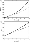 |
Fig. 8. Comparison of (a) radius of curvature and (b) minimum magnetic-field strength versus period for the old pendulum model (dashed line) and the corrected expression including the curvature of the solar surface (solid line) from Eq. (27). In this plot, we consider ρ = 2 × 10⁻¹⁰ kg m−3. |
The pendulum model also predicts a minimum value for the magnetic field strength of the prominence (Paper I) by assuming that the magnetic field supports the cool, dense prominence threads. As shown in Sect. 3.2, the magnetic tension is responsible for the support. Thus, according to Eq. (19), the magnetic tension is larger than the weight of the threads, such that
 (26)
(26)
Assuming that the slow-mode (gas-pressure gradient) contribution is small, Eq. (25) yields the following corrected relation:
 (27)
(27)
where Bold is defined by Eq. (7) in Paper I. The difference comes from the new term in the denominator. Figure 8b compares the minimum magnetic-field strength inferred from the corrected pendulum model with the values obtained with the uncorrected version. The discrepancy increases with the period; in fact, Eq. (27) shows that the corrected field strength increases asymptotically as P approaches P⊙. For periods longer than P⊙, the equation is not valid. However, for typical LALO periods (≤90 min; Luna et al. 2018), the discrepancies are small. As we noted previously (Luna et al. 2014), the density ρ introduces an important uncertainty in Eq. (27) unless ρ is directly measured, because the range of possible values is two orders of magnitude. Therefore, the uncertainty in the magnetic-field determination is much larger than the correction introduced by the nonuniform gravity, for typical LALO periods (P ∼ 1 h). For longer periods, however, the intrinsic spatial variations of the gravity might introduce comparable corrections.
6. Discussion and conclusions
In this work, we show that the longitudinal oscillations (magnetoacoustic-gravity modes) commonly observed in solar prominence threads are influenced by the intrinsic spatial variations of the solar gravity, which always points radially toward the solar center. This effect introduces a correction in the equations governing the longitudinal oscillations, and it modifies the pendulum-model approximation. This correction depends on the period and is evident from periods longer than 60 min. A new radius of curvature is defined as the combination of the dip radius of curvature and the solar-surface curvature. The gravity correction has another interesting effect. In order to support the prominence against gravity, the dips of the field lines must have concave-upward curvature; the limiting case is straight lines with no curvature. Hence, a cut-off period exists for longitudinal oscillations. Observed longitudinal oscillations always have periods below P < P⊙ = 167 min, which can be tested observationally. The largest longitudinal period reported so far is 160 min (Jing et al. 2006), very close to the cut-off. This confirms that the main restoring force is gravity and that the gas-pressure gradients make only small contributions to the oscillations. In addition, prominence oscillations with periods between 5 and 30 h have been detected (Pouget et al. 2006; Foullon et al. 2004, 2009). The existence of the cut-off period excludes the possibility that those oscillations are fundamental magnetoacoustic-gravity modes.
The pendulum model approximation assumes that the prominence dips are semicircular, for simplicity. In this work, we studied the influence of the dip geometry on magnetoacoustic-gravity modes by modeling flux tubes with semicircular, semielliptical, and sinusoidal dips. In all the cases, the period depends mainly on the radius of curvature at the bottom of the dip and not on the exact model considered. We found that the pendulum model is quite robust and is still valid for noncircular dips.
We also studied the influence of the new modified pendulum model on prominence seismology. The new model relates the oscillation period and the minimum magnetic-field strength to the radius of curvature at the bottom of the dips. We find that the magnetic-field correction is not very large for typical observed longitudinal oscillation periods of around one hour. However, for periods above 60 min the correction is significant. Zhang et al. (2017) reported a LALO event with a relatively long period of ≈99 min, yielding a radius of curvature of 244 Mm and a field intensity of 28 G under the original pendulum model. With the corrections discussed in this paper, the estimated radius of curvature is 376 Mm, and the field intensity is 35 G, differing substantially from the Zhang et al. values. More recently, Dai et al. (2021) also reported a LALO event with an even longer period of ≈120 min, from which they estimated a radius of curvature of 355 Mm and a field strength of 34 G with the old pendulum expression. With the corrected pendulum model the radius of curvature is 734 Mm and the field intensity is 49 G.
We conclude that the intrinsic spatial variations of the solar gravity introduce important corrections to the pendulum model. In addition, the corrected pendulum model provides a good estimate of the radius of curvature at the bottom of the dips for any flux-tube geometry. This work was limited to modeling linear motions in the oscillations, for which the center of mass of the cool prominence thread moves negligibly around the bottom of the dip. However, most longitudinal oscillations are classified as large amplitude, where the prominence thread is advected far from the dip center through regions with different curvatures. In order to achieve an in-depth understanding of the relationship between the period and the flux-tube geometry, this nonlinear behavior will be the subject of future research.
Acknowledgments
M.L. acknowledges support through the Ramón y Cajal fellowship RYC2018-026129-I from the Spanish Ministry of Science and Innovation, the Spanish National Research Agency (Agencia Estatal de Investigación), the European Social Fund through Operational Program FSE 2014 of Employment, Education and Training and the Universitat de les Illes Balears. This publication is part of the R+D+i project PID2020-112791GB-I00, financed by MCIN/AEI/10.13039/501100011033. J.T.K. was supported in part by NASA’s H-ISFM program. The authors also acknowledge support from the International Space Sciences Institute (ISSI) via team 413 on “Large-Amplitude Oscillations as a Probe of Quiescent and Erupting Solar Prominences”
References
- Arregui, I., Oliver, R., & Ballester, J. L. 2018, Liv. Rev. Sol. Phys., 15, 3 [Google Scholar]
- Dai, J., Zhang, Q., Zhang, Y., et al. 2021, ApJ, 923, 74 [NASA ADS] [CrossRef] [Google Scholar]
- Foullon, C., Verwichte, E., & Nakariakov, V. M. 2004, A&A, 427, L5 [NASA ADS] [CrossRef] [EDP Sciences] [Google Scholar]
- Foullon, C., Verwichte, E., & Nakariakov, V. M. 2009, ApJ, 700, 1658 [NASA ADS] [CrossRef] [Google Scholar]
- Goossens, M., Poedts, S., & Hermans, D. 1985, Sol. Phys., 102, 51 [NASA ADS] [CrossRef] [Google Scholar]
- Jing, J., Lee, J., Spirock, T. J., et al. 2003, ApJ, 584, L103 [NASA ADS] [CrossRef] [Google Scholar]
- Jing, J., Lee, J., Spirock, T. J., & Wang, H. 2006, Sol. Phys., 236, 97 [NASA ADS] [CrossRef] [Google Scholar]
- Leroy, J. L., Bommier, V., & Sahal-Brechot, S. 1983, Sol. Phys., 83, 135 [NASA ADS] [CrossRef] [Google Scholar]
- Liakh, V., Luna, M., & Khomenko, E. 2020, A&A, 637, A75 [NASA ADS] [CrossRef] [EDP Sciences] [Google Scholar]
- Liakh, V., Luna, M., & Khomenko, E. 2021, A&A, 654, A145 [NASA ADS] [CrossRef] [EDP Sciences] [Google Scholar]
- Luna, M., & Karpen, J. 2012, ApJ, 750, L1 [NASA ADS] [CrossRef] [Google Scholar]
- Luna, M., Díaz, A. J., & Karpen, J. 2012, ApJ, 757, 98 [Google Scholar]
- Luna, M., Knizhnik, K., Muglach, K., et al. 2014, ApJ, 785, 79 [NASA ADS] [CrossRef] [Google Scholar]
- Luna, M., Terradas, J., Khomenko, E., Collados, M., & Vicente, A. D. 2016a, ApJ, 817, 157 [NASA ADS] [CrossRef] [Google Scholar]
- Luna, M., Díaz, A. J., Oliver, R., Terradas, J., & Karpen, J. 2016b, A&A, 593, A64 [NASA ADS] [CrossRef] [EDP Sciences] [Google Scholar]
- Luna, M., Su, Y., Schmieder, B., Chandra, R., & Kucera, T. A. 2017, ApJ, 850, 143 [NASA ADS] [CrossRef] [Google Scholar]
- Luna, M., Karpen, J., Ballester, J. L., et al. 2018, ApJS, 236, 35 [NASA ADS] [CrossRef] [Google Scholar]
- Pouget, G., Bocchialini, K., & Solomon, J. 2006, A&A, 450, 1189 [NASA ADS] [CrossRef] [EDP Sciences] [Google Scholar]
- Priest, E. 2014, Magnetohydrodynamics of the Sun (Cambridge University Press) [Google Scholar]
- Ruderman, M. S., & Luna, M. 2016, A&A, 591, A131 [NASA ADS] [CrossRef] [EDP Sciences] [Google Scholar]
- Rust, D. M. 1967, ApJ, 150, 313 [NASA ADS] [CrossRef] [Google Scholar]
- Shen, Y., Liu, Y. D., Chen, P. F., & Ichimoto, K. 2014, ApJ, 795, 130 [Google Scholar]
- Terradas, J., Soler, R., Díaz, A. J., Oliver, R., & Ballester, J. L. 2013, ApJ, 778, 49 [Google Scholar]
- Terradas, J., Soler, R., Luna, M., et al. 2016, ApJ, 820, 125 [Google Scholar]
- Vršnak, B., Veronig, A. M., Thalmann, J. K., & Zic, T. 2007, A&A, 471, 295 [NASA ADS] [CrossRef] [EDP Sciences] [Google Scholar]
- Zhang, Q. M., Chen, P. F., Xia, C., & Keppens, R. 2012, A&A, 542, A52 [NASA ADS] [CrossRef] [EDP Sciences] [Google Scholar]
- Zhang, Q. M., Chen, P. F., Xia, C., Keppens, R., & Ji, H. S. 2013, A&A, 554, 124 [Google Scholar]
- Zhang, Q. M., Li, D., & Ning, Z. J. 2017, ApJ, 851, 47 [NASA ADS] [CrossRef] [Google Scholar]
All Figures
|
Fig. 1. Flux tube geometries considered in this work: (a) semicircular dip, (b) elliptical dip, and (c) sinusoidal dip. The solid line is the flux tube with the smallest radius of curvature. The dashed line is a case with a radius of curvature intermediate between the minimum and the maximum. In both Models 1 and 2, the end points of the flux-tube components change in order to keep the total length of the field line constant. |
| In the text | |
|
Fig. 2. Sketch of a dip with circular shape (solid line) with radius R. The red arrow shows the solar gravity on a point of the tube (𝒫) pointing to the center of the Sun, C⊙. |
| In the text | |
|
Fig. 3. Corrected pendulum period Eq. (18) as a function of the old pendulum period P0 (solid line). The dot-dashed line is plotted to show the diagonal where P = P0. We see that the period deviates from the diagonal for periods larger than 50 min. |
| In the text | |
|
Fig. 4. Corrected period (Eq. (17)) as a function of R (solid line). For comparison, the dashed line shows the uncorrected pendulum period P0. The horizontal dotted line shows the cut-off period P⊙, toward which P tends asymptotically. |
| In the text | |
|
Fig. 5. Period of fundamental-mode period found by solving Eq. (4) for Model 1 (solid line). The dotted line is the approximation given by Eq. (21), the dashed line shows the corrected pendulum period from Eq. (17), and the dot-dashed line is the uncorrected pendulum-model period P0. |
| In the text | |
|
Fig. 6. Eigenfunction v = v(s) solutions of Eq. (4) normalised to its maximum value for (a) circular, (b) elliptical, and (c) sinusoidal tube models (see Fig. 1). The thick black line corresponds to the mode with the minimum radius of curvature for each model (see Sect. 2.3), and the thick gray line corresponds to R0 = 1000 Mm. The thin lines correspond to eigenfunctions with intermediate R0 values, smoothly transitioning between both extreme functions. The two red dashed lines in (a) are the normal modes for both maxima and minima of R0 for the uniform-gravity case. |
| In the text | |
|
Fig. 7. Comparison of (a) period as a function of curvature radius at the bottom of the dip, R0, for the three geometries considered: Model 1 (solid line), Model 2 (circles), and Model 3 (diamonds). In (b) the comparison of the percentage of discrepancy between the exact period and that estimated by the corrected pendulum model (Eq. (17)) as a function of the exact period. |
| In the text | |
|
Fig. 8. Comparison of (a) radius of curvature and (b) minimum magnetic-field strength versus period for the old pendulum model (dashed line) and the corrected expression including the curvature of the solar surface (solid line) from Eq. (27). In this plot, we consider ρ = 2 × 10⁻¹⁰ kg m−3. |
| In the text | |
Current usage metrics show cumulative count of Article Views (full-text article views including HTML views, PDF and ePub downloads, according to the available data) and Abstracts Views on Vision4Press platform.
Data correspond to usage on the plateform after 2015. The current usage metrics is available 48-96 hours after online publication and is updated daily on week days.
Initial download of the metrics may take a while.