| Issue |
A&A
Volume 660, April 2022
|
|
|---|---|---|
| Article Number | A118 | |
| Number of page(s) | 16 | |
| Section | Planets and planetary systems | |
| DOI | https://doi.org/10.1051/0004-6361/202142583 | |
| Published online | 27 April 2022 | |
Emission from HCN and CH3OH in comets
Onsala 20-m observations and radiative transfer modelling
1
Department of Space, Earth and Environment, Chalmers University of Technology, Onsala Space Observatory,
43992
Onsala,
Sweden
e-mail: This email address is being protected from spambots. You need JavaScript enabled to view it.
2
European Southern Observatory,
Av. Alonso de Cordova
3107
Vitacura,
Santiago,
Chile
Received:
4
November
2021
Accepted:
1
February
2022
Abstract
Aims. The aim of this work is to characterise HCN and CH3OH emission from recent comets.
Methods. We used the Onsala 20-m telescope to search for millimetre transitions of HCN towards a sample of 11 recent and mostly bright comets in the period from December 2016 to November 2019. Also, CH3OH was searched for in two comets. The HCN sample includes the interstellar comet 2I/Borisov. For the short-period comet 46P/Wirtanen, we were able to monitor the variation of HCN emission over a time-span of about one month. We performed radiative transfer modelling for the observed molecular emission by also including time-dependent effects due to the outgassing of molecules.
Results. HCN was detected in six comets. Two of these are short-period comets and four are long-period. Six methanol transitions were detected in 46P/Wirtanen, enabling us to determine the gas kinetic temperature. From the observations, we determined the molecular production rates using time-dependent radiative transfer modelling. For five comets, we were able to determine that the HCN mixing ratios lie near 0.1% using contemporary water production rates,  , taken from other studies. This HCN mixing ratio was also found to be typical in our monitoring observations of 46P/Wirtanen but here we notice deviations of up to 0.2% on a daily timescale which could indicate short-time changes in outgassing activity. From our radiative transfer modelling of cometary comae, we find that time-dependent effects on the HCN level populations are of the order of 5–15% when
  is around 2 × 1028 mol s−1. The effects may be stronger for comets with lower
  . The exact details of the time-dependent effects depend on the amount of neutral and electron collisions, radiative pumping, and molecular parameters such as the spontaneous rate coefficient.
Key words: comets: general / radio lines: general
© ESO 2022
1 Introduction
Most comets are expected to be remnants from the early times, some 4.5 billion years ago, when the Solar System was formed, and therefore may contain records of the chemical and physical properties of these times past. Exceptions to this notion are the recent discoveries of the objects 1I/’Oumuamua and 2I/Borisov which are suggested to be interstellar visitors entering our Solar System with strongly hyperbolical and thus unbound trajectories. When approaching the Sun to within a few astronomical units (au), comets can start to sublimate molecules and other volatile particles from their surfaces and form what is known as a cometary coma. Studying the composition of the content of cometary comae can therefore reveal information about the physical conditions and chemistry prevailing when the Solar System was born or that of similar systems in the solar neighbourhood in the case of interstellar visitors.
Studies of the molecular content of cometary comae are performed either by remote sensing (mainly by recording spectral signatures over a wide range of wavelengths from radio to the ultraviolet regimes) or by in situ measurements made by spacecraft like Giotto (1P/Halley) and, more recently, Rosetta (67P/Churyumov-Gerasimenko). As pointed out by Rubin et al. (2019), most abundances of the volatile content, as determined by these various means over the last 40 yr, are reminiscent of those in the interstellar medium (ISM) and thus suggest a chemical origin in interstellar, star-forming material. The major gaseous constituent of the neutral inner coma is water molecules, and the abundances of other species relate to water via the mixing ratio. For instance, the next two most abundant species, CO2 and CO, constitute typically 10–20% of that of water (Mumma & Charnley 2011; Rubin et al. 2019). Further out in the coma, the solar radiation will affect the composition. At 1 au from the Sun, the outgassing water molecules are photodissociated into H and OH at a rate of about (1–2) x 10−5s−1 (Huebner et al. 1992) where the factor of two variation reflects the degree of solar activity. Another water-destruction mechanism is pho-toionization into H2O+, which is about 30 times slower. This latter process, together with photoionization of OH, previously formed from water, is the main source of electrons in the coma (Rubin et al. 2009). As water is relatively difficult to spectro-scopically observe, several other, indirect methods have been employed to determine the water production rate. Firstly, observations of the photodissociation product OH can be used as a proxy for water (Despois et al. 1981; Bonev et al. 2006). Secondly, observations of the remaining H, via Ly-α, can also be used as exemplified by the Solar Wind ANisotropies (SWAN) Ly-a camera observations on board the SOlar and Heliospheric Observer (SOHO) spacecraft (e.g. Combi et al. 2011). A third indirect method is to use a relatively abundant parent species, like HCN, as an indicator of water; see Mumma & Charnley (2011) for an overview. Direct observations of the ground-state water lines are scarce and are mostly limited to satellites (e.g. Lecacheux et al. 2003; Lis et al. 2013; Biver et al. 2015). Infrared spectroscopy of the ro-vibrational water lines has proven useful in determining the water production rates (Mumma et al. 2003). This latter method, albeit relying on fluorescence pumping models, has the advantage that the excitation conditions can be determined via a rotation temperature, and consequently provide more accurate production rates (e.g. DiSanti et al. 2016). Lastly, in situ measurements by spacecraft via high-resolution mass spectroscopy provide perhaps the most direct way to probe the molecular coma content, although this method is limited to only a few comets (e.g. Läuter et al. 2020).
The observations presented in this paper are part of an ongoing effort to study comets at millimetre (mm) wavelengths using the Onsala Space Observatory (OSO) 20-meter telescope. This effort was initiated by Wirström et al. (2016) who presented HCN(1-0) observations of the long-period comets C/2013 R1 (Lovejoy) and C/2014 Q2 (Lovejoy). We expand this study here with observations of another 12 comets. The observational efforts focus primarily on using HCN(1–0) as an indicator of water, but one comet, 46P/Wirtanen, was also observed in methanol. Both of these molecules are believed to be released from nucleus ices (Dello Russo et al. 2016). Our comet target sample comprises bright comets with perihelion dates from late 2016 to 2019. The sample includes comets belonging to the Jupiter family as well as the Oort cloud. In addition, we searched for HCN towards 2I/Borisov. Furthermore, we also investigate possible caveats – in terms of time-dependent radiative transfer effects – that may complicate the interpretation of the observed emission from HCN (as well as from other molecules) in cometary comae.
This paper is structured as follows. In the following section, we describe the observations made with the OSO 20-m telescope. In Sect. 3 we present the results and in Sect. 4 we outline the radiative transfer analysis made in which we also take into account time-dependent aspects. After discussing our results in Sect. 5, we finally present our conclusions.
Observed lines.
2 Observations
All observations presented in this paper were made from late 2016 until late 2019 using the radome-enclosed OSO 20-m antenna equipped with the 3 mm channel of the 3 and 4 mm receiver system (Belitsky et al. 2015). The radome allows us to observe sources near the Sun without thermal distortion of the telescope optics. The rest frequencies of the target lines (see Table 1) were covered by two frequency tunings, one centred near 88 GHz and the other near 96 GHz. All tunings were performed in the velocity frame of the comet. Coordinates and velocities of all comets were taken from the Horizons system1 (Giorgini et al. 1996) tabulated every hour and then interpolated by the observing system. The antenna half-power beam width is 40 arcsec at the HCN frequency and about 37 arcsec for the CH3OH observations.
The Fast Fourier Transform Spectrometers (FFTSs) were configured into a wide 4-GHz mode or a narrow 156 MHz mode. In both modes, the two linear polarizations are recorded separately. The wide 4-GHz mode is made up of two partly overlapping 2.5 GHz FFTSs of 32768 channels and was used for the CH3OH observations and part of the HCN observations. The wide mode results in a velocity resolution of about 0.25 km s−1. The narrow 156 MHz setup was routinely used for the HCN observations. The observations were made in frequency switching mode with a frequency throw for the HCN setup of 5 MHz for data taken in 2016–2017 and 7 MHz from 2018 onwards. When observing CH3OH, the wide spectrometer setup was employed to cover all lines (see Table 1) and the used frequency throw was larger, 25 MHz, to avoid line confusion.
The weather conditions varied during our observations. In the best conditions, the system temperature was around 120 K. Typically the measurements were automatically halted when the system temperature became large, around 800–1200 K. Pointing and focus optimisations were performed several times a day using the SiO 2–1 v = 1 maser line at 86 GHz towards stars. Measurements from 2018 onwards were made with the new antenna control system developed by M. Lerner and called BIFROST2, which provides an improved and more automated control of remote observations. We used these capabilities to perform pointings and to refocus automatically every three hours and to automatically pause observations when the system temperature rose above 800 K. We used 60 and 120 s integrations for individual scans. With the switch to BIFROST we employed observing blocks consisting of fifteen 60-s scans with hot-load calibrations between every fifth scan.
Information on the 12 comets investigated in this study is summarized in Table 2 where the range of observing dates, total integration time, heliocentric distance, Rh, distance to Earth, ∆, and variations over the observing dates are also listed. The projected nucleocentric distance (near the centre of the date range), d, as subtended by the beam size for HCN(1–0) transition is also listed.
Observed comets with the OSO 20-m telescope.
Observed HCN intensities and upper limits.
3 Results
The HCN and CH3OH observations are displayed in Figs. 1–7. The shown spectra have been smoothed to a resolution of 0.3 km s−1 (except the 46P/Wirtanen global average spectrum) and intensities are shown in Tmb-scale. The individual scans were first folded before being noise-weighted to form an average. Because of the frequency-switching observing mode, a rather high-order polynomial was needed to subtract the baseline. The used baseline order was typically from 3 to 7 where the higher orders were used for the observations with larger frequency throws. The channel RMS and integrated line intensities, Imb, have been entered in Table 3. Errors and upper limits are 1σ in this table. The variation of errors and limits among the comets is a combination of system temperature and integration time. The integrated line intensity of HCN(J = 1 → 0) is calculated as a sum of the three hyperfine structure (hfs) line intensities (listed in Table 1) using a box of 2 km s−1 in width centred on each hfs line. The 46P/Wirtanen monitoring measurements are listed in Table 4 as a function of UT date and modified Julian date (MJD). Below we give a short introduction and summary of the results for each comet observed:
C/2016 U1 (NEOWISE). This comet (hereafter U1), discovered in October 2016 by the Near-Earth Object Wide-field Infrared Survey Explorer (NEOWISE), follows a slightly hyperbolic orbit (eccentricity just above 1). At perihelion on 14 January 2017 its heliocentric distance was 0.32 au. The spectrum presented in Fig. 1 is the average over four observing dates ranging from 22 December 2016 to 10 January 2017. This object was not detected in HCN and the upper limit of the integrated intensity is listed in Table 3.
45P/Honda-Mrkos-Pajdušáková. This short-period comet discovered in 1948, and hereafter referred to as 45P, belongs to the Jupiter family and has a period of 5.26 yr. The water production was estimated by Dello Russo et al. (2020) to be (2–3) × 1027 mol s−1 using infrared spectroscopy in mid-February 2017. The same study reports an HCN production rate of (3–4) × 1024 mol s−1. On 16 February 2017, there was also a CN outburst seen (Springmann et al. 2019). We did not detect the HCN 1–0 triplet; see Fig. 1. The bulk of our HCN data was obtained early February 2017.
2P/Encke. This short-period comet was observed several times in the first half of March 2017. Our HCN observations resulted in a non-detection. Later in March, after perihelion, the water production rate was estimated to be (3–4) × 1028 mol s−1 and the HCN production rate was (3–6) × 1025mol s−1 (Roth et al. 2018).
41P/Tuttle-Giacobini-Kresák. This comet was first observed in 1858 and later rediscovered in 1907 and 1952 as pointed out by Schleicher et al. (2019). Like 45P, this comet (hereafter 41P) belongs to the Jupiter family and has a period of 5.42 yr. In early April 2017 its peak water production rate was 3.5 × 1027mols−1 (Moulane et al. 2018). The 41P nucleus rotation underwent an unusually large slow-down with a rotation period increasing from 20 h in March 2017 to more than 50 h in early May (Schleicher et al. 2019). Our April 2017 HCN 1–0 detection at the 4.6σ level is shown in Fig. 1.
C/2015 ER61 (PanSTARRS). This comet, hereafter ER61, follows a highly eccentric orbit and is suggested to originate in the inner Oort cloud (Meech et al. 2017). The OSO 20-m HCN 3.7σ detection is shown in Fig. 2. The spectrum is an average over three observing days in 2017: 6, 11, and 22 April. The observations took place after ER61 underwent an outburst on 4 April (Opitom et al. 2019). Sekanina (2017) suggests that the flare-up was caused by fragmentation of the nucleus creating a companion nucleus which was observed later in June. Our observations on 9 May were disregarded because of an inaccurate set of ephemerides. Saki et al. (2021) report a water production rate of around 1 × 1029 mol s−1 in mid-April 2017 and an HCN rotational temperature near 70 K. This is consistent with the Ata-cama Large Millimeter/Submillimeter Array (ALMA) compact array HCN observations in mid-April by Roth et al. (2021b). Both studies determined the HCN production rate to be near 9 × 1025mols−1.
C/2017 E4 (Lovejoy). This long-period comet (referred to as E4) appears to have originated in the inner Oort Cloud (Faggi et al. 2018). Our observations took place on 7 April and resulted in an upper limit; see Fig. 2. Faggi et al. (2018) reported a water production rate of about 3 × 1028 mol s−1 and an HCN production rate of about 5 × 1025 mol s−1 only 3 days before our observations took place. The comet disintegrated in late April 2017.
C/2015 V2 (Johnson). This Oort cloud comet (OCC), here-after referred to as V2, follows a slightly hyperbolic orbit and was observed during one observing run stretching from 18-19 May in 2017 before the perihelion on 12 June. These observations resulted in an HCN 3.9σ detection; see Fig. 2. Combi et al. (2021) estimated water production rates from SOHO/SWAN observations but to the best of our knowledge no other direct molecular studies of V2 are found in the literature for this period of time.
C/2017 O1 (ASASSN1). This long-period comet, hereafter referred to as O1, is a possible Manx comet (Brinkman 2020), which is a category of tail-less long-period comets that may have formed in the inner Solar System before being ejected to the outskirts. Our observation, resulting in a 7.4σ detection (Fig. 2), took place in two shifts in mid-October 2017 (12/13 and 14/15).
96P/Machholz. This short-period comet has a rather peculiar high-inclination, low-perihelion orbit, being a Jupiter-family comet (JFC). Its nucleus is thought to be inactive (e.g. Eisner et al. 2019). Our observations, of CH3OH only, were made when 96P/Machholz was at a heliocentric distance of 0.16 au on 30 October 2017 (the perihelion distance was 0.12 au for the 2017 apparition). Emission from CH3OH was not detected with the OSO 20-m at this date, see Fig. 3, and the upper limit for the Jk = 20–10 A+ line has been included in Table 5.
46P/Wirtanen. This JFC was the only comet in our sample that could be monitored in HCN; see Fig. 5 and Table 4. The first detection of HCN was made on 9 December 2018 and the last detection was made on 18 January 2019. The detection level was better than 3σ except on the dates 10 December and 10 January. On 20 December, we detected the strongest HCN line intensity. The HCN spectrum of this date is shown in Fig. 4. CH3OH was also clearly detected, and the spectrum (an average of data taken between 22 and 28 December) is shown in Fig. 6. Six different methanol lines around 96 GHz are seen (Table 5), each at a detection level of 5σ or better. 46P/Wirtanen came very close to Earth in December 2018 (0.08 au) and was therefore widely observed3. In addition, it showed much higher activity than during previous apparitions (Farnham et al. 2019). HCN was observed by Wang et al. (2020) (J = 1–0) and Coulson et al. (2020) (J = 4–3). The latter study also included J = 7–6 CH3OH data. A week before its closest approach to Earth, Roth et al. (2021c) observed the J = 5–4 CH3OH lines using the ALMA array. These authors found variable CH3OH outgassing consistent with the rotational period of 9 h (Farnham et al. 2021) of the nucleus. In December 2018, Biver et al. (2021) performed a molecular survey of 46P mainly using the Institut de RadioAs-tronomie Millimétrique (IRAM) 30-m telescope but also the NOrthern Extended Millimeter Array (NOEMA). At perihelion (12.9 December 2018), Moulane et al. (2019) reported a water production rate of 7.2 × 1027mol s−1 followed by a number of other infrared spectroscopy studies (Saki et al. 2020; Roth et al. 2021a; Bonev et al. 2021; Khan et al. 2021; McKay et al. 2021) as well as submillimetre observations of
 (Lis et al. 2019).
C/2018 Y1 (Iwamoto). This bright and long-period comet, hereafter called Y1, came close (0.4 au) to Earth in February 2018. On February 5, DiSanti et al. (2019) report H2O and HCN production rates of 2 × 1028 mol s−1 and 4 × 1025 mol s−1, respectively. By averaging data between 10 and 19 February we obtained a very clear 9σ detection of HCN; see Fig. 7. Data taken on February 4 were excluded in the analysis because of erroneous Doppler corrections.
2I/Borisov. Being only the second interstellar object known to have visited our Solar System, it was the first such object to show outgassing activity. This was confirmed in September 2019 (Fitzsimmons et al. 2019). From interferometry imaging observations using ALMA (Cordiner et al. 2020) and Hubble Space Telescope (HST) observations (Bodewits et al. 2020), a CO-production rate of about (5–10) × 1026 mol s−1 around perihelion was found. Cordiner et al. (2020) also determined the HCN production rate to be 7 × 10²³mol s−1. The 20-m observations in October and November 2018 only resulted, when averaging all data, in an upper limit of the HCN 1-0 emission; see Fig. 7.
In the cases of 46P/Wirtanen (both HCN and CH3OH) and C/2018 Yl (Iwamoto), we see slightly shifted profiles in the sense that their peaks appear shifted with ~0.3–0.4km s−1 to lower velocities; see Figs. 4, 6, and 7. This apparent blueshift likely indicates that the gas outflow component directed towards Earth is more pronounced. As both these comets were at Rh> 1 au at the time of our observations, much of their sunward sides were then facing Earth. To illustrate this asymmetry more clearly, a global average of all HCN high-resolution data for 46P/Wirtanen is also shown in Fig. 4 for which the blue peak is centred at –0.4 ± 0.1 km s−1 when fitted with a Gaussian. The ratio of the blue to red wing emission for this spectrum is 2.6 ± 0.2 when using the velocity ranges ±(0.15–0.85) km s−1 for the strongest JF = 12–01 line. The observed line widths for 46P and Yl seem to indicate an expansion velocity of between 0.5 and 0.6 km s−1.
46P/Wirtanen HCN 2018/19 monitoring results.
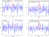 |
Fig. 1 OSO 20-m HCN 1–0 spectra towards the comets U1, 45P, 2P/Encke, and 41P. The velocity scale is in the reference frame of the comets and the intensity scale is in Tmb. The positions of the three hfs components are marked with red bars. The relative heights of the bars correspond to the statistical weights, gu, in Table 1. The integrated intensity is also shown together with 1σ error or as 1σ- upper limit where applicable. |
4 Radiative transfer modelling of comets
As mentioned above, water is the main ingredient in the volatile material that is being outgassed from the comet surface. The gaseous material leaves the comet surface with a nearly constant expansion velocity ve. Further out in the coma, the water molecules may be photoionized into H2O+ and photodissociated mainly into OH and H (Rubin et al. 2009). Other molecules, like HCN, behave in a similar way. In addition, HCN is an important precursor to CN (Fray et al. 2005; Paganini et al. 2010) although heated CN-bearing dust could be a significant source of gaseous CN according to Hänni et al. (2020). This pure gas expansion may of course be modified when for example ions start to deflect when interacting with the solar wind. This happens near what is called the contact surface, RCS (Rubin et al. 2009). However, the radial distribution of neutral parent molecules (i.e. those with origin from the comet surface) is thought to follow the Haser relation (Haser 1957):
 (1)
(1)
as a function of cometocentric radius r, where Qmol is the molecular production rate and γP is the photodissociation rate at the distance to the Sun.
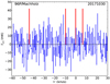 |
Fig. 3 CH3OH spectrum towards the comet 96P/Machholz on 30 October 2017. The positions where the CH3OH lines would appear are indicated by the red bars. Scales are as in Fig. 1. |
4.1 Basic equations
As pointed out by Crovisier & Le Bourlot (1983), the change rate of the physical conditions, like density decline due to expansion, in the cometary comae is not significantly different from the scale of molecular (in this case CO) radiative and collisional rates, although their relative importance varies with radius. Here, we mainly follow the approach by Chin & Weaver (1984), Bockelée-Morvan et al. (1984), Crovisier (1987), and Bockelée-Morvan (1987) when setting up the basic equations governing the excitation.
For simplicity, we start with a two-level system with upper level population nu and lower level population n1. The total population is n = nu + n1. The population change for the two levels can be expressed as the differential equations (DEs):
 (2)
(2)
 (3)
(3)
where Aul is the spontaneous decay from u to l and BulJv and BluJv are the rates due to stimulated emission and absorption, respectively, when exposed to the averaged radiation field Jv at the frequency v. The downward and upward collisional rates are denoted cul and clu, respectively. These are the standard processes included for a two-level system. We have also added two other destruction rates referred to as γu and γl These could for example represent destruction due to photodissociation or pho-toionization. We hereafter assume that the destruction rate is equal for the upper and lower levels, that is, we set γ = γu = γ1. By adding Eqs. (2) and (3), we then obtain
 (4)
(4)
which simply tells us that the total population n(t) is exponentially decaying with time (if γ > 0).
In the case of a cometary coma, due to the outgassing, the molecules expand with a velocity according to ve, which we assume to be constant here. The cometocentric radius, r, is then given as r = rc + vet as a function of time. The radius of the comet nucleus is rc. The destruction rate can then be modified to
 (5)
(5)
where γp is the destruction rate due to photodissociation (or photoionization) and the second term, 2ve/r, reflects the population dilution due to constant expansion. We note that the first part in Eq. (5) allows an expansion velocity varying with radius. However, hereafter we always assume a constant gas expansion velocity. By changing át to dr/ve in Eqs. (2) and (3), it is straightforward to rewrite the population changes as a function of r instead of t. For instance, Eq. (4) then becomes
 (6)
(6)
which solves into the Haser distribution, Eq. (1), when integrated. Hence, by adopting this approach we can study possible time-dependent effects of the individual level populations nu and n1 as a function of cometocentric radius by solving the DEs in Eqs. (2) and (3) while still maintaining an overall decline due to the Haser equation. This may be of particular interest near the contact surface (RCS) where the electron properties vary very rapidly (they enter into the equations via cul and clu).
The above two-level system of equations is easily generalised into a multi-level system, but in order to simplify the solution of the DEs we here neglect the contribution from the line itself when calculating the averaged radiation field,  at any given radial point in the coma. We assume that the contributions to
  only come from the diluted black body radiations of the comet nuclei, the Sun, and the 2.7 K cosmic background, respectively. Here we use the geometric dilution factors for the comet nuclei, βc(r), and that for the Sun,β⊙. The remaining fraction of the 4π sky background is assumed to be filled by the Tcmb = 2.7 K cosmic background radiation. Neglecting effects due to shadowing, this can be expressed as
![Mathematical equation: ${\bar J_v} = {\beta_{\rm{c}}}(r)J({T_{\rm{c}}}) + {\beta_ \odot}J({T_ \odot}) + \left[{1 - {\beta_{\rm{c}}}(r) - {\beta_ \odot}} \right]J\left({{T_{{\rm{cmb}}}}} \right).$](/articles/aa/full_html/2022/04/aa42583-21/aa42583-21-eq12.png) (7)
(7)
Here, J(T) = 1/(exp(hv/kT) −1), where h and k are Planck’s and Boltzmann’s constants, respectively. The radiation temperatures used are the surface temperature of the comet, Tc, and for the Sun we use T⊙ = 5772 K (Hertel & Schulz 2015). The geometric dilution factor for the Sun, β⊙, at 1 au is about 5 × 10⁻⁶ and at the surface of the comet we have that β⊙(rc) = 1/2. We have not included thermal radiation from dust particles in the modelling presented here.
In order to solve the DEs, Eqs. (2) and (3), we adopt initial population values at t = 0 and r = rcthat are appropriate to the production rate,  , and the initial excitation is entirely governed by the temperature of the comet surface, Tc. Following Bensch & Bergin (2004), we adopt a constant neutral gas kinetic temperature in the coma cloud set to the Tc value. We note that this is a simplification and some adiabatic cooling can take place (Biver et al. 2015). We use a fourth-order Runge-Kutta scheme (Abramowitz & Stegun 1972) when solving the DEs, adapting the step size because of the radial gradients. The coma model cloud is assumed to be spherically symmetric. At any radius, we can also determine level populations in the statistical equilibrium (SE) case similar to Paganini et al. (2010) by only including radiative and collisional processes.
We are only modelling HCN and CH3OH comet emission in this study. The overall photo-dissociation and photoioniza-tion rates for HCN, CH3OH, and H20 (given at 1 au from the quiet Sun) used come from the compilation by Huebner et al. (1992) which, for the molecules considered here, are essentially the same as those listed in the more recent work by Huebner & Mukherjee (2015). Depending on the heliocentric distance Rh of the comet, these are scaled by (1/Rh)2. Furthermore, we assume Rh to be constant during the solution.
To properly account for collisional excitation we include collisions by electrons and H20 molecules. While the molecule–electron collisions are relatively easy to determine, collisions by water molecules are much more difficult to compute. For instance, it is only very recently that collisional rate coefficients for the collision systems CO-H20 (J ≤ 10) were determined accurately (Faure et al. 2020). In the case of HCN (with hyper-fine structure) and CH3OH, no such calculations exist yet. Limited (J < 8) HCN-H2O collisional rate coefficients have been determined by Dubernet & Quintas-Sánchez (2019) which are being used here together with the HCN-He rates of Dumouchel et al. (2010) for higher J (J ≥ 8). The latter rates were scaled to approximately match the J < 8 HCN-H2O rates before being concatenated to the Dubernet & Quintas-Sánchez (2019) rates. For CH3OH, we use the CH3OH-H2 rates of Rabli & Flower (2010) (for para H2). We treat the methanol A- and E-species separately and do not include excited torsional states. The neutral collisional rates used are those valid for a kinetic temperature, Tk, of 50 K and then simply scaled with (Tk/50 K)1/2 for other temperatures. We use the tabulated downward collisional rates and calculate the corresponding upward rates from detailed balance. For HCN-e collisional rates, we adopt those determined by Faure et al. (2007) and for the electron excitation of CH3OH we use a set of rates computed in the Born approximation.
Normally, to speed up the calculations, we only include energy levels below 150–250 K for HCN and CH3OH. The exact cut-off depends on the temperature. However, we have the option to include higher energy levels for testing if there are any truncation problems. Furthermore, vibrationally excited levels (v2) for HCN can also be fully included. However, the situation with a large number of levels together with levels with small populations requires much smaller step sizes to maintain the solution accuracy throughout the coma. This makes the computation very time consuming and a much faster way is to include effective pumping rates (see Paganini et al. (2010); Bensch & Bergin (2004)), via the v1, v2, 2v2, and v3 vibrational states. We only include the P- and R-branches for the ro-vibrational HCN transitions here because they can cause redistribution of the ground-state level populations in the outer coma (e.g. Bockelée-Morvan 1987). The Q-branch (∆J = 0) transitions do not do that by themselves (when neglecting rotational relaxations within the excited state). This way of incorporating effective pumping rates, adopting the radiation field in Eq. (7), is only valid when a small fraction of the molecules are in the excited states. This is typically the case for HCN (Bockelée-Morvan et al. 1984). We have not used any pumping rates for CH3OH in our modelling here.
To fully quantify the collisional processes as a function of cometocentric radius, not only the collisional rates are needed but also the radial distributions of water molecules and electrons. The water distribution is assumed to follow the Haser equation (Eq. (1)) assuming a water production rate  . The water production rate can be connected to the molecular (HCN or CH3OH) production rate Qmol via the abundance ratio
  , which is normally referred to as the mixing ratio. To quantify the electron density radial distribution, ne(r), we adopt the approach by Bensch & Bergin (2004) who based their formulation on the work by Biver (1997) (see also Zakharov et al. 2007). Bensch & Bergin (2004) express ne(r) (and electron temperature) in terms of the water production rate and like Paganini et al. (2010) we use
  as the density scaling factor. The rather complex radial behaviour of the electron density and temperature is visualised by Bensch & Bergin (2004) in their Fig. 1.
The solution of the time-dependent radiative transfer is in practice accomplished by a Python code called comrad.py. This code is adapted to read molecular data files used in the Leiden atomic and molecular database (Schöier et al. 2005) and is slightly modified to also include photo-destruction values in the Solar radiation field at 1 au (Huebner et al. 1992) and a section of IR pumping transitions (for HCN P- and R-branches between the ground state and the excited states v1, v2, 2v2, and v3). The frequencies and A-coefficients of the IR pumping transitions are taken from the HITRAN molecular database (Gordon et al. 2017). After the molecular level populations have been determined as a function of cometocentric radius, we obtain the modelled spectra, assuming a constant expansion velocity and a turbulent velocity width, by convolving the projected radial intensity distribution with a Gaussian appropriate to the telescope beam size and the comet distance (∆). Although the HCN level populations are strongly affected in the outer coma by the IR pumping transitions, the impact on the resulting line intensities of ground-state rotational transitions is small because the major contribution comes from regions of high density (this can be pronounced by smaller observing beams).
In Appendix A we investigate the effects of the time-dependent radiative transfer calculations by comparing the results to those of steady-state SE calculations. We use the time-dependent radiative transfer model described above in the analysis of our HCN and CH3OH data and the results of the modelling are described in the following section.
Observed CH3OH intensities and upper limit.
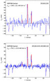 |
Fig. 4 Top: HCN 1–0 spectrum towards the comet 46P/Wirtanen on 20 December 2018. The positions, corresponding to a frequency throw of 7 MHz, of the negative artifacts of the HCN lines have been marked with negative dashed red lines. Bottom: global average of all high-resolution (0.1 km s−1) HCN data observed from 20 December 2018 to 18 January 2019. Scales are as in Fig. 1. |
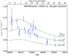 |
Fig. 5 OSO 20-m HCN 1–0 monitoring data towards 46P/Wirtanen in December 2018 and January 2019. The data points (blue marker with vertical lσ errors bars; horizontal bars indicate the range of observations), which are also listed in Table 4, represent the integrated intensity as a function of MJD or days from perihelion. The dashed lines represent the results from the radiative transfer modelling (see Sect. 4) using three different HCN production rates from 0.5 × 1025mol s−1 to 1.5 × 1025 mol s−1 as indicated for a temperature of 70 K and |

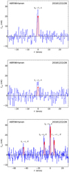 |
Fig. 6 OSO 20-m methanol spectra towards 46P/Wirtanen when averaging data between 22 and 28 December 2018. The red spectra represent the modelling results of the radiative transfer modelling (see Sect. 4) using a CH3OH production rate of 1.6 × 1026 mol s−1 and a kinetic temperature of 70 K. |
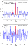 |
Fig. 7 Top: OSO 20-m HCN 1–0 spectrum towards C/2018 Yl (Iwamoto). It is an average of data between 10 and 19 February 2019. Bottom: HCN spectrum observed towards 2I/Borisov in October/November 2019. Scales are as in Fig. 1. |
Properties of the comets and results of the HCN modelling.
4.2 Model results
Our HCN modelling results are summarised in Table 6. Here, the properties used for each comet (46P/Wirtanen only 20 December 2018) are also listed. The adopted nucleus radius, rc, which serves as a starting point for the model calculation, is also included but has essentially no impact on the modelling results. For 46P and Y1, we obtained the expansion velocities from the line widths. This results in 0.55 km s−1 for both comets. Coulson et al. (2020) found a similar value of ~0.6 km s−1 for 46P (at Rh = 1.06 au). We note that, for 45P, Lovell et al. (2017) report an outflow velocity of about 0.8 km s−1 from OH observations (at Rh = 0.54 au). Biver et al. (2006) determined a relation of ve and heliocentric distance (in au):  . This relation yields expansion velocities near 1.3 km s−1 for 2P/Encke and around 0.55 km s−1 for 2I/Borisov. The observed ve around 0.55 km s−1 for 46P and Y1 lie below this relation. For 46P and Y1, the above relation predicts 0.76 and 0.70 km s−1, respectively. However, for the other comets we use an expansion velocity according to this relation.
In the case of U1 and O1, we cannot find representative water production rates in the literature. Here, we instead used the mean value of  from Bockelée-Morvan & Biver (2017) to determine an appropriate
  for the modelling. It should be noted that the derived QHCN does not depend strongly on the adopted
  (as verified below by the 46P results where a factor of two increase in
  results in a 7% increase in the required QHCN).
When possible we also use published values for the gas temperature (which is also used for the neutral gas kinetic temperature here and Te out to RCS) as indicated in the table. The kinetic temperature is clearly dependent on the heliocentric distance Rh and Biver et al. (1997) estimated the kinetic temperature of C/1995 O1 (Hale-Bopp) from CH3OH (and CO) observations as a function of Rh to be around 100 K at 1 au and approximately scaling as Rh−1 with heliocentric distance. In the case of 46P/Wirtanen, we use our CH3OH observations to estimate the kinetic temperature; see below. If a kinetic temperature estimate is lacking, we used 60 K for comets with Rh ≥ 1.3 au and 70 K for the remaining comets in the model calculations. These values approximately reflect the temperature behaviour as a function of heliocentric distance found by Biver et al. (1999) for C/1992 B2 (Hyakutake) or by DiSanti et al. (2016) in the case of D/2012 S1 (ISON). The temperature estimates used in Table 6 sometimes stem from rotational temperatures of molecules like H2O or CH3OH. How well this rotational temperature reflects the gas kinetic temperature of the major collision agent (H2O) depends on the degree of thermalisation. Also, collisions by electrons may change the excitation of the molecular probe (Xie & Mumma 1992).
Because of the observed blueshifted line profiles for 46P/Wirtanen and also C/2018 Y1 (Iwamoto), it is likely that there is an anisotropic distribution of QHCN in the sense that the production rate is higher on the sunward side of the comet than on the anti-sunward side (with a factor of 2–3 difference, see Fig. 4). This was also noted by Wang et al. (2020) and Biver et al. (2021) for HCN and for CH3OH by Roth et al. (2021c). Our modelled values, which are based on a spherically symmetric model geometry, therefore refer to an average production rate.
As mentioned above, in the case of 46P/Wirtanen, we can estimate the gas kinetic temperature because we detect lines with quite different upper energies (as high as 83 K). Another aspect of CH3OH transitions, which is due to the nuclear spin directions of the methyl group H atoms, is that they come in two different symmetry species, A and E, which are, as pointed out by Bockelée-Morvan et al. (1994), radiatively and collisionally uncoupled apart from possible line overlaps. The lowest E-state is about 8 K above the lowest A-state. Depending on the formation mechanism, they may be produced in unequal amounts. This can be the case at low temperatures (e.g. Wirström et al. 2011). If the temperature appropriate for methanol formation in comets is larger than 8 K, then we expect the production rates of the A- and E-species of CH3OH to be equal. We performed a grid testing with temperatures ranging from 40 to 120 K (in steps of 10 K) and  from 1.0 × 1026 mols−1 to 3.0 × 1026 mols−1 (in steps of 0.1 × 1026 mols−1). The water production rate used was
  which is an average of the
  determined by Combi et al. (2020) for the dates 22–28 December 2018. The grid combination of kinetic temperature and
  that gave the best fit (as indicated by smallest χ2-value) to the observed integrated intensities in Table 5 was for a temperature of 70 + 15 K and
  or 1.6% of the water production rate.
The fitting also indicated, within the errors, that the CH3OH A- and E-species are being outgassed in equal amounts in 46P/Wirtanen. The resulting model spectra are shown in Fig. 6 together with the observed spectra.
As noted above, the CH3OH modelling of 46P/Wirtanen resulted in a kinetic temperature of 70 K. Using this temperature and  which is the 22 December value of Combi et al. (2020), we find that for the 20 December data an HCN production rate of (1.6 + 0.1) x 1025mols−1 matches the observed integrated intensity; see Tables 6 and 4. Using a fixed value for the ratio
  of 0.1%, as found for the 20 December data, we ran models for three different HCN production rates at different dates and entered the expected 1–0 integrated intensity in Fig. 5. The production rates are (0.5,1.0,1.5) × 1025mols−1 which encompass most of the observed line intensities. Also included in Table 6 is the HCN production rate when adopting a lower water production rate as indicated by the infrared spectroscopy results (e.g. Bonev et al. 2021) a few days prior to 20 December. The change in QHCN is less than 10%. The individual HCN production rates (see Table 4) are shown in Fig. 8 together with the water production rates obtained using SOHO/SWAN by Combi et al. (2020). These results are discussed in the following section.
Our CH3OH observations of 96P/Machholz only resulted in an upper limit; see Table 5. Adopting Tc = 90 K and  , this upper limit corresponds to a very high methanol production rate. We estimate the upper limit production rate to be above 1028 mol s−1. The poor constraint of
  is due to the fact that 96P was only at Rh = 0.12 au at the time of the measurements and the size of the neutral coma is considerably smaller because of the effective destruction of H2O and CH3OH molecules near the Sun.
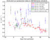 |
Fig. 8 HCN and H20 production rates in 46P/Wirtanen as a function of days from perihelion (12.9 December 2018 UT). The HCN rates (blue) were determined from the intensities (only those detected above the 3σ- level) in Table 4. The water production rates (red) contemporary with our QHCN results, are from Combi et al. (2020). The perihelion value of |

5 Discussion
In this section, we first discuss the previously determined HCN production rates as well as the upper limits. We also discuss the HCN production rates as an indirect indicator of water production rates via mixing ratios. In the case of 46P/Wirtanen, the monitoring results can be used to see variations in the HCN production rates on timescales of 1 day and these are compared to other observations of HCN and H20 production rates. Our usage of methanol as a thermal probe is also discussed. Finally, our time-dependent treatment of the radiative transfer of comets is discussed in relation to a more standard approach performed in the steady-state limit of the SE assumption.
5.1 HCN production rates
As can be seen in Table 6, we detected HCN in two JFCs (41P and 46P, the latter comet is discussed in more detail in the following section) and four long-period OCCs (ER61, V2, O1, and Y1). For the six comets with HCN detections, the determined HCN production rates fall in the range (0.5–8) × 1025mols−1 and there is no obvious difference between the two types of comets. For the five comets where we also have independent (and reasonably contemporary) water production rates, the HCN to H2O mixing ratios are in the range 0.08–0.13%. This range of mixing ratios is consistent with the values as determined from radio observations and discussed by Mumma & Charnley (2011) and by Bockelée-Morvan & Biver (2017). However it is smaller than the typical value in Dello Russo et al. (2016) by a factor of about two. The latter study, based on high-resolution infrared spectroscopy, compiles a typical range of mixing ratios of 0.150.27%. Our ratios, near 0.1% for 41P, ER61, V2,46P, and Y1, are outside this range but are well above the lower extreme value of 0.03% found by Dello Russo et al. (2016).
In the case of 41P, our HCN data were obtained over a longer period in April 2017. The average water production rate derived from OH observations by Moulane et al. (2018) over this period is estimated to be about 3.5 × 1027mols−1 with no larger variations. Moulane et al. (2018) also report CN production rates in the range (4–5) × 1024mols−1 which is similar to our HCN production rate of (4.5 ± 1.0) × 1024 mol s−1. This could indicate that the CN radicals observed in 41P mainly stem from photodis-sociation of HCN. However, given the uncertainties and that our QHCN is an average (over time and over the coma), one cannot exclude a contribution to QCN from dust grains as suggested by Dello Russo et al. (2016) and Hänni et al. (2020).
The ER61 observations (HCN and H2O) by Saki et al. (2021) occurred on three occasions in our 6–22 April observation range and here we adopt an average of their water production rates of 1 × 1029 mol s−1. These authors deduced HCN mixing ratios in the range 0.11–0.14%, somewhat higher than our value of 0.082%. This is possibly due to the fact that our HCN data reflect a larger time-span. However, the ALMA results (Roth et al. 2021b) indicate an HCN mixing ratio (0.072%) consistent with our value.
For Y1, the used water production rate of DiSanti et al. (2019) dates from about a week before our estimate of the HCN production rate. Adopting this  , the mixing ratio is 0.10 ± 0.02%. DiSanti et al. (2019) obtain an HCN mixing ratio of 0.2% on 4 February 2018. This could indicate variations in
  if we assume that the HCN production rate is constant over this period of observations.
In the case of the remaining HCN detections, V2 and O1, no other directly determined molecular production rates have been found to date in the literature. However, for V2, Combi et al. (2021) estimated the water production rate using SOHO/SWAN observations to about 4 × 1028 mol s−1 near our observation date. The corresponding mixing ratio is about 0.08%. We also note that Venkataramani & Ganesh (2018) reported on the absence of molecular emissions towards V2 at Rh = 2.83 au but they noted that such emissions appeared later on a low level when Rh = 2.3 au. Our 3.9σ detection was made at Rh = 1.67 au.
In five of our observed comets (U1, 45P, 2P/Encke, E4, and 2I/Borisov), we only obtained upper limits on QHCN; see Table 6. At the time of writing, no molecular observational results for U1 have been reported in the literature and so here we have nothing to compare to. The HCN production rate of (3–4) × 1024 mol s−1 in 45P found by Dello Russo et al. (2020) refers to dates in mid-February 2017. Our non-detection, QHCN < 3.2 × 1024mols−1, is from early February and indicates that the production rate of HCN was about the same or lower in early February. Roth et al. (2018) observed HCN in 2P/Encke after perihelion on 21 and 25 March, resulting in QHCN ~ (3–6) × 1025mols−1. Our upper limit only indicates that QHCN, before and around perihelion, did not exceed 6–8 times this value. For E4, Faggi et al. (2018) determined an HCN production rate of 5 × 1025 mol s−1. This was 3 days before we obtained an upper limit of 6 × 1025 mol s−1 and so apparently there was no significant increase in QHCN from April 4 to 7. Our upper limit on QHCN towards 2I/Borisov is consistent with the ALMA HCN detection on 14 and 15 December by Cordiner et al. (2020). They determined that QHCN = 7 × 10²³ mols−1. Taken together, based on our J = 1−0 data, the HCN mixing ratios seem to fall near 0.1% when we have reasonably contemporary estimates of  .
.
5.2 Variation in the HCN production rates for 46P/Wirtanen
We determined HCN production rates for 46P/Wirtanen (Table 4) from a few days before perihelion until 36 days after perihelion; see Figs. 5 and 8. There are clear variations in QHCN, sometimes on a daily basis, but it is also evident that QHCN has decreased by a factor of 2–3 some month after the perihelion passage. We note that Wang et al. (2020) observed HCN 1–0 on 14–15 December and obtained a QHCN (based on LTE calculations) of about half our value and that the IRAM 30-m observations (Biver et al. 2021) on 14 December result in a QHCN in between our value (1.4 × 1025 mol s−1) and that of Wang et al. (2020). A few days later, in the range 15–17 December, the IRAM 30-m data show QHCN determinations very close to our values. The James Clerk Maxwell Telescope (JCMT) HCN(4–3) data of Coulson et al. (2020) showed little daily variation in QHCN in the period 15 December to the early UT hours of 20 December. The HCN production rates determined by Wang et al. (2020), Biver et al. (2021) and Coulson et al. (2020) are all included in Fig. 8. The HCN(4–3) QHCN results agree relatively well with our results up until 20 December. Here we see a clear increase in QHCN to (1.6 ± 0.1) × 1025 mol s−1 by a factor of two over that from Coulson et al. (2020). However, the JCMT observations relate to the early UT hours and our observations are from about 12 h later on the same day. This would indicate an outburst event during the day of 20 December. However, early on 21 December the zero-spacing NOEMA observations of Biver et al. (2021) again indicate a lower QHCN of 0.8 × 1025mols−1, meaning that if there was an outburst it must have been rather short (≲ 12 h) so as not to be recorded by the NOEMA observations. In fact, similar changes of  by about a factor of two were seen by Roth et al. (2021c), connecting it to the rotation period timescale of 9 h.
Based on infrared spectroscopy, Bonev et al. (2021) reported an HCN production rate of (1.47 ± 0.07) × 1025mols−1 on 17 December. This QHCN is significantly higher than our value of (0.9 ± 0.2) x 1025 mol s−1 and the value (0.7 ± 0.1) × 1025 mol s−1 of Coulson et al. (2020) from the same date. Four days later, on 21 December, Khan et al. (2021) observed HCN, also by infrared spectroscopy. Their HCN production rate averaged to about 1.3 × 1025 mol s−1 which is near our value of 1.1 × 1025 mol s−1 (see Table 4) on the same date. The QHCN values from Bonev et al. (2021) and Khan et al. (2021) have been included in Fig. 8.
As already pointed out in Sect. 4.2, there appears to be a clear difference of a factor of two to three in the outgassing activity on the sunward versus anti-sunward parts of the comet nucleus over the course of about one month. As reported by Biver et al. (2015), based on their water line observations by the Microwave Instrument for the Rosetta Orbiter (MIRO) of the JFC 67P/Churyumov-Gerasimenko, the nightside water production rate was low, <1% of the dayside production rate (at rh = 3.4 au). Later, at rh = 1.8 au, Fink et al. (2016) report for 67P that about 17% of the total water production emerges from the nightside. In any case, this is a higher day-to-nightside activity ratio than we see for 46P but our ratio is averaged over a period of a month in which the daytime fraction as seen by our telescope beam changed (elongation varied from 160 to 140deg from 20 December 2018 to 18 January 2019).
The SOHO/SWAN monitoring observations (Combi et al. 2020) to estimate  in 46P coincide partly in time with our observations and provide estimates of the water production rate variation. As these results are based on Ly-α observations of the hydrogen coma (dissociation product from H2O and OH), they refer to an average water production of the 2–3 days prior to the actual observation date (as indicated by the horizontal error bars in Fig. 8) and so the
  determined this way may not probe activity variations on shorter timescales. However, the trend we see in QHCN from 20 December until 18 January (8–36 days after perihelion) is consistent with a mixing ratio near 0.1%. For the week preceding this time-span, Biver et al. (2021) report almost the same value 0.11 ± 0.01%. There are a few QHCN estimates in our monitoring time-span 8-36 days after perihelion that seem to indicate an HCN mixing ratio near 0.2%. This is also the case for the pre-perihelion observations. To distinguish whether this reflects real changes in the mixing ratio by a factor of about two or is an effect of different time-averaging would require
  measurements with ~1 day time-resolution or better. If it is an effect of time-averaging, the HCN production rate will be a good indicator of the water production rate in the case of 46P/Wirtanen. The increase in QHCN seen by us on 20 December seems supported by the large water production rate reported by Combi et al. (2020) 2–3 days later and, as discussed earlier, the QHCN reported by Khan et al. (2021) on 21 December but not by the NOEMA observations in the early UT hours on 21 December.
5.3 Coma gas kinetic temperature and methanol production in 46P/Wirtanen
In Sect. 4.2, we determined the gas kinetic temperature of 46P from methanol data taken over the time-span 22–28 December to be 70 ± 15 K. Furthermore, the deduced production rate of  corresponds to a methanol mixing ratio of about 1.6%. Our mixing ratio is very near the JFC average value of 1.7% as compiled by Dello Russo et al. (2016) and slightly less than the JFC median value of about 2% as compiled by Mumma & Charnley (2011).
Most other methanol observations of 46P refer to the period around the perihelion or the week after. For instance, on 7 –9 December, Roth et al. (2021c) used ALMA observations to determine methanol rotation temperatures in the range from 50 to 80 K. Using IRAM 30-m CH3OH observations, Biver et al. (2021) determined six-day averages (over the range 12–18 December) of the gas temperature in the range 53–75 K. On 16 December, Coulson et al. (2020) used the JCMT to observe three methanol lines around 338 GHz. They determined the rotation temperature to Trot ~ 30–50 K. Using infrared spectroscopy observations on 18 December, Roth et al. (2021a) report a methanol rotation temperature of about 90 K. In addition, Biver et al. (2021) also made a single methanol observation on 25.8 December 2018 UT – within our observing time range –, which resulted in a gas temperature of 43 ± 7 K.
Three studies estimate H2O rotation temperatures of 46P. On 14 and 19 December, Saki et al. (2020) determined the water rotation temperature to be about 85 K. On 18 December, Roth et al. (2021a) report a rotation temperature of about 90 K. Later, on 21 December Khan et al. (2021) derived temperatures of 80 K to 90 K. Our derived value of the gas kinetic temperature of about 70 K, as averaged over 22–28 December, is consistent with the studies mentioned above. There is a possibility that the temperature decreased from 80–90 K to about 40–50 K during our observations (cf. Khan et al. 2021; Biver et al. 2021). However, this notion is somewhat complicated by the variation of temperature estimates (30–90 K) prior to our observations.
In the case of the methanol production in 46P, we begin with noting that on 7–9 December, the ALMA CH3OH observations (Roth et al. 2021c) resulted in varying CH3OH production rates in the range (2.0−3.6) – 1026mols−1. The IRAM 30-m data by Biver et al. (2021) determined  to (2.6 ± 0.2) × 1026 mol s−1 averaged over 12–18 December. The JCMT observations on 16 December (Coulson et al. 2020) resulted in (3.5 ± 0.2) × 1026 mols−1. On 18 December, Roth et al. (2021a) report a methanol production rate around 2 × 1026 mol s−1. A few days later, on 21 December, Khan et al. (2021) reported a similar methanol production rate of 2.5 × 1026 mol s−1. These estimates of
  are all higher than our later, 22–28 December value of
  . The NOEMA observations (Biver et al. 2021) on 25.8 December 2018 UT resulted in (1.84 ± 0.14) × 1026 mols−1, which is close to our value.
As noted above, we adopt  which is an average of the
  determined by Combi et al. (2020) for the dates 22–28 December 2018. This
  results in a mixing ratio of 1.6%. For the two-week period prior to our methanol observations, mixing ratios in the range 2–5% were reported (Roth et al. 2021c; Biver et al. 2021; Coulson et al. 2020; Roth et al. 2021a; Khan et al. 2021). Based on this, we suggest that the average methanol mixing ratio decreased by about a factor of two from around perihelion into our observing period of 22–28 December.
The production rates of the methanol A- and E-species are about equal for 46P within the uncertainties. This would suggest a temperature environment of ≳8 K during the formation of the methanol molecules. Finally, the determined kinetic temperature is related to the used CH3OH-H2O collisional rate coefficients which in our case were based on the CH3OH-H2 rates. As already pointed out, accurate collisional rate coefficients currently only exist for the collision systems CO-H2O (Faure et al. 2020) and HCN-H2O (Dubernet & Quintas-Sánchez 2019).
5.4 Time-dependent radiative transfer versus SE calculations
To study time-dependent effects, we used fragment B of 73P as a test case (see Appendix A) and we noted that the HCN level populations deviated by 5–15% (for J = 0−5) when comparing the time-dependent results with the steady-state SE-calculations. The water production rate for 73P/B is around 2 × 1028 mol s−1. We also found that the time-dependent deviations would be larger for comets with lower water production rates, because the collisions with water molecules will be less frequent in the inner part of the coma. Likewise, by reducing the effect of electron-HCN collisions, the time-dependent effects became more pronounced. For molecules with lower electric dipole moments (and hence generally lower A-coefficients), we expect the effects to be more pronounced, at least in the outer coma where radiative processes dominate (see Fig. A.1). However, strong IR-pumping could counteract the effect in the outer coma, making the details of the excitation picture very complicated. We expect the influence of time-dependent effects on the HCN level populations to be small (≲20%) for  .
.
It is worth pointing out that the total molecular population is bound to follow the radial Haser distribution so that molecular production rates based on the analysis of a larger number of transitions should be less affected by the time-dependent effects encountered here. Also, the present modelling work neglects excitation effects at a certain position in the coma caused by line radiation from other parts of the coma (same as assuming optically thin radiation in the level population determination). This may be a good approximation for most cometary molecular probes but an important exception is water excitation (e.g. Bockelée-Morvan 1987; Bensch & Bergin 2004). Extending our model to using an escape probability formalism (cf. Gersch & A'Hearn 2014) is a possibility, but would require an iterative solution technique; that is, solving for the entire coma using an initial guess (using the DE here or simply an SE solution), including the line radiation in Eq. (7), and then repeating the procedure with time-dependent solutions throughout the coma until the level populations converge. Presumably, this would be a very time-consuming technique but could be tried for water excitation in comets. Solution methods based on the Monte Carlo technique (Bernes 1979) or those using accelerated lambda iteration (Rybicki & Hummer 1991; Bergman & Humphreys 2020) appear to be less suitable for time-dependent studies because they rely on the SE steady state assumption. However, in the escape probability formalism (e.g. Bockelée-Morvan 1987; van der Tak et al. 2007; Zakharov et al. 2007), the A-coefficients are replaced by βA where β is the (local) escape probability for the transition in question. In the case of optically thick transitions (β ~ 1/τ), this could imply that time-dependent effects due to a reduction in radiative excitation could be of greater importance.
Another aspect is that, because the radiative transfer formulation here is in the time domain, it would be easier to incorporate chemical and photolytic state-to-state reactions when solving excitation of several molecules at the same time in the coma. Finally, it is worth stressing that most radiative transfer models, including the one presented here, assume a spherically symmetric coma geometry. Remote observations and in situ studies of cometary comae clearly show deviations from this geometry and models like that of Debout et al. (2016) could be used for studying time-dependent effects also in anisotropic comae.
6 Summary and conclusions
We performed spectral line observations of HCN and CH3OH transitions towards a sample of bright comets using the OSO 20-m telescope. From the observations, we determined molecular production rates using a radiative transfer model taking into account time-dependent effects. Our main conclusions can be summarised as follows. – We detected HCN(1–0) in six comets of our sample: two JFCs and four OCCs. For five of these comets, we were able to determine the HCN mixing ratio using published values of  The determined HCN mixing ratios were all near 0.1% (0.08−0.013%).
We detected HCN emission in 46P/Wirtanen on 21 occasions from 9 December 2018 to 18 January 2019. When comparing with contemporary
 determinations, we find a typical mixing ratio near 0.1% with possible variations of up to 0.2%. This variation can also be due to short-time activity variations (≲1 d) not reflected in the Ly-α observations used for determining
  . We also noted a clear asymmetry in the observed HCN and CH3OH line profiles in the sense that the sunward activity was about a factor of two to three stronger than the outgassing activity on the 46P night-side.
In addition to HCN, we detected six CH3OH transitions in 46P/Wirtanen around two weeks after perihelion in December 2018. This enabled us to determine the gas kinetic temperature to be about 70 K. The methanol mixing ratio was found to be 1.6%, which is about half that of the methanol mixing ratio during the two weeks prior to our observations.
To interpret our HCN and CH3OH observations, we used a radiative transfer code in which we allowed for time-dependent effects on the level populations by relaxing the normal steady-state assumption of statistical equilbrium (SE) in the cometary coma. In our test case (73P fragment B, see Fig. A.2) we noticed 5–15% deviations of the HCN level populations as compared to SE values. We recognized that the time-dependent effects may be more pronounced for comets with lower water production rates and if the molecular excitation via electron collisions becomes less efficient. For
 , the time-dependent effects in the HCN excitation should be small.
Acknowledgements
We are very grateful to L. Paganini for sharing his HCN modelling details. We also thank N. Biver for making his 1997 thesis available to us. The Onsala Space Observatory national research infrastructure is funded through Swedish Research Council grant No 2017-00648.
Appendix A Validation of the time-dependent model
As a starting point for the validation of our time-dependent model described in Sect. 4, we adopt the case for comet 73P/Schwassmann-Wachmann, hereafter 73P, which broke into fragments during its 2006 apparition. Paganini et al. (2010) observed the HCN J = 3 − 2 and J = 4 − 3 lines in 73P on May 12, 2006, using the Heinrich Hertz Submillimeter Telescope (HHSMT). Contemporary Caltech Submillimeter Observatory (CSO) HCN observations of 73P/B were also made (Lis et al. 2008). Paganini et al. (2010) also performed comprehensive modelling of the HCN emission to which we can compare our modelling results. We adopt the values for the fragment B that these authors used: QHCN = 3 × 1025mols−1,  , T = 90K, and ve = 0.53 km s−1. To further mimic their setup, we neglect hfs and include effective pumping rates. In the upper panel of Fig. A.1 we show the HCN fractional level populations for J = 2,3,4 as a function of cometocentric radius.
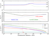 |
Fig. A.1 Time-dependent HCN modelling with parameters corresponding to the fragment B of 73P/Schwassmann-Wachmann. The upper plot shows the fractional level populations for levels J = 2,3,4 as a function of cometocentric distance. The middle plot shows the relative importance of different downward rates for the HCN J = 3 − 2 transition. As indicated, the included rates are radiative (excluding IR pumping rates), and collisional rates both for electrons and water molecules. The sum of these rates is included as a black line. They are normalized with the time-dependent rate due to destruction and constant expansion; see Eq. (5). The bottom panel depicts the radial density variations. The blue curve is the total HCN density and the green curve represents the water density behaviour. The electron density, ne(r), is drawn in red. Also the HCN/H2O ratio is shown. It is not entirely flat, because when the photodissociation becomes important in the outer coma, HCN and H2O molecules are destroyed with slightly different rates. |
The appearance of the level population variation looks very similar to that of Fig. 1 in Paganini et al. (2010), suggesting that any time-dependent effects are not significant in this particular case. Our late time values are about a factor 1.2-1.5 larger than those of Paganini et al. (2010). The middle panel in this figure depicts the relative importance of the different HCN excitation mechanisms (for J = 3 − 2). In the inner coma, collisions with water molecules are most important, while in the outer coma, radiative processes dominate. It between, as shown by Xie & Mumma (1992), collisions by electrons are the most important excitation mechanism.
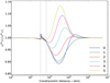 |
Fig. A.2 HCN level (J = 0 to 5) population variation as a function of cometocentric radius, for the time-dependent modelling (see Fig. A.1) adopting the parameters for fragment B of 73P/Schwassmann-Wachmann during its 2006 passage. The level populations have been normalised to their SE-values to visualise time-dependent effects. The vertical dotted lines correspond to radii RCS and 2RCS between which the electron temperature increases from 90 K to 104 K. |
The different downward rates in the middle panel of Fig. A.1 have been normalised with the rate due to expansion and destruction, γ in Eq. (5). When this ratio is around 1 or smaller, we may see time dependency effects. As visualised in the bottom panel of Fig. A.1, where the radial density variations of water, HCN, and electrons are shown, the electron properties change very rapidly at the contact surface radius, RCS = 324 km. Here the electron temperature Te rises very steeply from the comet temperature to around 104 K (Ip 1985; Bensch & Bergin 2004), accompanied with an increase in electron density.
It is around a cometocentric radius near RCS (see the middle panel in Fig. A.1) where we should start to see the time-dependent effects on the excitation (cf. Chin & Weaver 1984). To investigate this in more detail, we display in Fig. A.2 the ratio of the time dependent level populations (J = 0 to 5) to those valid in the SE-limit. The level population ratios are very close to 1 up to about r = 100 km (cf. Bockelée-Morvan et al. 1984) and from radii larger than about r = (4 − 5) × 104 km. After the sharp increase in Te from 90 K to 104 K over the interval [RCS, 2RCS], the level populations deviate from the SE-values during the settling – in this case at most up to 7% for J = 2. The low-J level populations settle a little later than the high-J level populations because their A-coefficients are smaller. This deviation is not directly related to the change in electron properties but to that of the normalized rates (see middle panel in Fig. A.1), which are close to 1. Due to its large electric dipole moment, HCN rotational transitions have large A-coefficients and we expect that for molecules with smaller spontaneous rates (e.g. CO), the settling of the level populations will take place further out in the coma. The deviations from the SE populations will be larger if  is reduced because HCN-H2O collisions will be less effective in settling the populations. For instance, using
  in our test case, the time-dependent J = 2 population deviations reach 9% and for
  they are at the 5% level. By reducing the number of electron collisions (by lowering
  from 0.3 to 0.15) the effects are less clear. Firstly, the initial time-dependent deviation at RCS will be less pronounced but the settling at larger radii, 103 − 104 km, will show larger deviations. Increasing the number of electron collisions will reduce the slower time-dependent behaviour (and increase the deviation at RCS).
References
- Abramowitz, M., & Stegun, I. A. 1972, Handbook of Mathematical Functions (New York: Dover) [Google Scholar]
- Belitsky, V., Lapkin, I., Fredrixon, M., et al. 2015, A&A, 580, A29 [NASA ADS] [CrossRef] [EDP Sciences] [Google Scholar]
- Bensch, F., & Bergin, E. A. 2004, ApJ, 615, 531 [NASA ADS] [CrossRef] [Google Scholar]
- Bergman, P., & Humphreys, E. M. L. 2020, A&A, 638, A19 [NASA ADS] [CrossRef] [EDP Sciences] [Google Scholar]
- Bernes, C. 1979, A&A, 73, 67 [NASA ADS] [Google Scholar]
- Biver, N. 1997, PhD thesis, Université Paris 7, France [Google Scholar]
- Biver, N., Bockelée-Morvan, D., Colom, P., et al. 1997, Earth Moon Planets, 78, 5 [NASA ADS] [CrossRef] [Google Scholar]
- Biver, N., Bockelée-Morvan, D., Crovisier, J., et al. 1999, AJ, 118, 1850 [NASA ADS] [CrossRef] [Google Scholar]
- Biver, N., Bockelée-Morvan, D., Crovisier, J., et al. 2006, A&A, 449, 1255 [NASA ADS] [CrossRef] [EDP Sciences] [Google Scholar]
- Biver, N., Hofstadter, M., Gulkis, S., et al. 2015, A&A, 583, A3 [NASA ADS] [CrossRef] [EDP Sciences] [Google Scholar]
- Biver, N., Bockelée-Morvan, D., Boissier, J., et al. 2021, A&A, 648, A49 [EDP Sciences] [Google Scholar]
- Bockelée-Morvan, D. 1987, A&A, 181, 169 [Google Scholar]
- Bockelée-Morvan, D., & Biver, N. 2017, Phil. Trans. R. Soc. London, Ser. A, 375, 20160252 [Google Scholar]
- Bockelée-Morvan, D., Crovisier, J., Baudry, A., et al. 1984, A&A, 141, 411 [Google Scholar]
- Bockelée-Morvan, D., Crovisier, J., Colom, P., & Despois, D. 1994, A&A, 287, 647 [Google Scholar]
- Bodewits, D., Noonan, J. W., Feldman, P. D., et al. 2020, Nat. Astron., 4, 867 [Google Scholar]
- Boehnhardt, H., Riffeser, A., Ries, C., Schmidt, M., & Hopp, U. 2020, A&A, 638, A8 [NASA ADS] [CrossRef] [EDP Sciences] [Google Scholar]
- Bonev, B. P., Mumma, M. J., DiSanti, M. A., et al. 2006, ApJ, 653, 774 [NASA ADS] [CrossRef] [Google Scholar]
- Bonev, B. P., Dello Russo, N., DiSanti, M. A., et al. 2021, Planet. Sci. J., 2, 45 [NASA ADS] [CrossRef] [Google Scholar]
- Brinkman, C. L. 2020, AAS Meeting Abs., 454.02 [Google Scholar]
- Chin, G., & Weaver, H. A. 1984, ApJ, 285, 858 [NASA ADS] [CrossRef] [Google Scholar]
- Combi, M. R., Bertaux, J. L., Quémerais, E., Ferron, S., & Mäkinen, J. T. T. 2011, ApJ, 734, L6 [CrossRef] [Google Scholar]
- Combi, M. R., Mäkinen, T. T., Bertaux, J. L., Quémerais, E., & Ferron, S. 2019, Icarus, 317, 610 [NASA ADS] [CrossRef] [Google Scholar]
- Combi, M. R., Mäkinen, T., Bertaux, J. L., et al. 2020, Planet. Sci. J., 1, 72 [Google Scholar]
- Combi, M. R., Shou, Y., Mäkinen, T., et al. 2021, Icarus, 365, 114509 [CrossRef] [Google Scholar]
- Cordiner, M. A., Milam, S. N., Biver, N., et al. 2020, Nat. Astron., 4, 861 [Google Scholar]
- Coulson, I. M., Liu, F.-C., Cordiner, M. A., et al. 2020, AJ, 160, 182 [Google Scholar]
- Crovisier, J. 1987, A&AS, 68, 223 [NASA ADS] [Google Scholar]
- Crovisier, J., & Le Bourlot, J. 1983, A&A, 123, 61 [NASA ADS] [Google Scholar]
- Debout, V., Bockelée-Morvan, D., & Zakharov, V. 2016, Icarus, 265, 110 [NASA ADS] [CrossRef] [Google Scholar]
- Dello Russo, N., Kawakita, H., Vervack, R. J., & Weaver, H. A. 2016, Icarus, 278, 301 [NASA ADS] [CrossRef] [Google Scholar]
- Dello Russo, N., Kawakita, H., Bonev, B. P., et al. 2020, Icarus, 335, 113411 [NASA ADS] [CrossRef] [Google Scholar]
- Despois, D., Gerard, E., Crovisier, J., & Kazes, I. 1981, A&A, 99, 320 [Google Scholar]
- DiSanti, M. A., Bonev, B. P., Gibb, E. L., et al. 2016, ApJ, 820, 34 [NASA ADS] [CrossRef] [Google Scholar]
- DiSanti, M., Saki, M., Gibb, E., et al. 2019, EPSC-DPS Joint Meeting, 2019, 822 [Google Scholar]
- Dubernet, M. L., & Quintas-Sánchez, E. 2019, Mol. Astrophys., 16, 100046 [NASA ADS] [CrossRef] [Google Scholar]
- Dumouchel, F., Faure, A., & Lique, F. 2010, MNRAS, 406, 2488 [NASA ADS] [CrossRef] [Google Scholar]
- Eisner, N. L., Knight, M. M., Snodgrass, C., et al. 2019, AJ, 157, 186 [NASA ADS] [CrossRef] [Google Scholar]
- Faggi, S., Villanueva, G. L., Mumma, M. J., & Paganini, L. 2018, AJ, 156, 68 [NASA ADS] [CrossRef] [Google Scholar]
- Farnham, T. L., Kelley, M. S. P., Knight, M. M., & Feaga, L. M. 2019, ApJ, 886, L24 [NASA ADS] [CrossRef] [Google Scholar]
- Farnham, T. L., Knight, M. M., Schleicher, D. G., et al. 2021, Planet. Sci. J., 2, 7 [Google Scholar]
- Faure, A., Varambhia, H. N., Stoecklin, T., & Tennyson, J. 2007, MNRAS, 382, 840 [Google Scholar]
- Faure, A., Lique, F., & Loreau, J. 2020, MNRAS, 493, 776 [NASA ADS] [CrossRef] [Google Scholar]
- Fink, U., Doose, L., Rinaldi, G., et al. 2016, Icarus, 277, 78 [Google Scholar]
- Fitzsimmons, A., Hainaut, O., Meech, K. J., et al. 2019, ApJ, 885, L9 [Google Scholar]
- Fray, N., Bénilan, Y., Cottin, H., Gazeau, M. C., & Crovisier, J. 2005, Planet. Space Sci., 53, 1243 [NASA ADS] [CrossRef] [Google Scholar]
- Gersch, A. M., & A’Hearn, M. F. 2014, ApJ, 787, 36 [NASA ADS] [CrossRef] [Google Scholar]
- Giorgini, J. D., Yeomans, D. K., Chamberlin, A. B., et al. 1996, AAS/Div. Planet. Sci. Meeting Abs., #28, 25.04 [Google Scholar]
- Gordon, I. E., Rothman, L. S., Hill, C., et al. 2017, J. Quant. Spectr. Rad. Transf., 203, 3 [Google Scholar]
- Hänni, N., Altwegg, K., Pestoni, B., et al. 2020, MNRAS, 498, 2239 [Google Scholar]
- Haser, L. 1957, Bulletin de la Societe Royale des Sciences de Liege, 43, 740 [NASA ADS] [Google Scholar]
- Hertel, I. V., & Schulz, C.-P. 2015, Atoms, Molecules and Optical Physics 2 (Berlin, Heidelberg: Springer) [Google Scholar]
- Howell, E. S., Lejoly, C., Taylor, P. A., et al. 2017, AAS/Div. Planet. Sci. Meeting Abs., #49, 414.24 [Google Scholar]
- Huebner, W. F., & Mukherjee, J. 2015, Planet. Space Sci., 106, 11 [Google Scholar]
- Huebner, W. F., Keady, J. J., & Lyon, S. P. 1992, Ap&SS, 195, 1 [NASA ADS] [CrossRef] [Google Scholar]
- Ip, W. H. 1985, Adv. Space Res., 5, 233 [NASA ADS] [CrossRef] [Google Scholar]
- Khan, Y., Gibb, E. L., Bonev, B. P., et al. 2021, Planet. Sci. J., 2, 20 [NASA ADS] [CrossRef] [Google Scholar]
- Läuter, M., Kramer, T., Rubin, M., & Altwegg, K. 2020, MNRAS, 498, 3995 [Google Scholar]
- Lecacheux, A., Biver, N., Crovisier, J., et al. 2003, A&A, 402, L55 [NASA ADS] [CrossRef] [EDP Sciences] [Google Scholar]
- Lis, D. C., Bockelée-Morvan, D., Boissier, J., et al. 2008, ApJ, 675, 931 [NASA ADS] [CrossRef] [Google Scholar]
- Lis, D. C., Biver, N., Bockelée-Morvan, D., et al. 2013, ApJ, 774, L3 [NASA ADS] [CrossRef] [Google Scholar]
- Lis, D. C., Bockelée-Morvan, D., Güsten, R., et al. 2019, A&A, 625, L5 [NASA ADS] [CrossRef] [EDP Sciences] [Google Scholar]
- Lovell, A. J., Amason, C., Howell, E. S., et al. 2017, AAS/Div. Planet. Sci. Meeting Abs., 49, 420.04 [Google Scholar]
- McKay, A. J., DiSanti, M. A., Cochran, A. L., et al. 2021, Planet. Sci. J., 2, 21 [NASA ADS] [CrossRef] [Google Scholar]
- Meech, K. J., Schambeau, C. A., Sorli, K., et al. 2017, AJ, 153, 206 [NASA ADS] [CrossRef] [Google Scholar]
- Moulane, Y., Jehin, E., Opitom, C., et al. 2018, A&A, 619, A156 [NASA ADS] [CrossRef] [EDP Sciences] [Google Scholar]
- Moulane, Y., Jehin, E., José Pozuelos, F., et al. 2019, EPSC-DPS Joint Meeting, 2019, 1036 [Google Scholar]
- Müller, H. S. P., Thorwirth, S., Roth, D. A., & Winnewisser, G. 2001, A&A, 370, L49 [Google Scholar]
- Mumma, M. J., & Charnley, S. B. 2011, ARA&A, 49, 471 [NASA ADS] [CrossRef] [Google Scholar]
- Mumma, M. J., DiSanti, M. A., Dello Russo, N., et al. 2003, Adv. Space Res., 31, 2563 [NASA ADS] [CrossRef] [Google Scholar]
- Opitom, C., Yang, B., Selman, F., & Reyes, C. 2019, A&A, 628, A128 [NASA ADS] [CrossRef] [EDP Sciences] [Google Scholar]
- Paganini, L., Villanueva, G. L., Lara, L. M., et al. 2010, ApJ, 715, 1258 [NASA ADS] [CrossRef] [Google Scholar]
- Paradowski, M. L. 2020, MNRAS, 492, 4175 [NASA ADS] [CrossRef] [Google Scholar]
- Pickett, H. M., Poynter, R. L., Cohen, E. A., et al. 1998, J. Quant. Spectr. Rad. Transf., 60, 883 [Google Scholar]
- Rabli, D., & Flower, D. R. 2010, MNRAS, 406, 95 [Google Scholar]
- Roth, N. X., Gibb, E. L., Bonev, B. P., et al. 2018, AJ, 156, 251 [NASA ADS] [CrossRef] [Google Scholar]
- Roth, N. X., Bonev, B. P., DiSanti, M. A., et al. 2021a, Planet. Sci. J., 2, 54 [Google Scholar]
- Roth, N. X., Milam, S. N., Cordiner, M. A., et al. 2021b, ApJ, 921, 14 [NASA ADS] [CrossRef] [Google Scholar]
- Roth, N. X., Milam, S. N., Cordiner, M. A., et al. 2021c, Planet. Sci. J., 2, 55 [NASA ADS] [CrossRef] [Google Scholar]
- Rubin, M., Hansen, K. C., Gombosi, T. I., et al. 2009, Icarus, 199, 505 [NASA ADS] [CrossRef] [Google Scholar]
- Rubin, M., Altwegg, K., Balsiger, H., et al. 2019, MNRAS, 489, 594 [Google Scholar]
- Rybicki, G. B., & Hummer, D. G. 1991, A&A, 245, 171 [NASA ADS] [Google Scholar]
- Saki, M., Gibb, E. L., Bonev, B. P., et al. 2020, AJ, 160, 184 [Google Scholar]
- Saki, M., Gibb, E. L., Bonev, B. P., et al. 2021, AJ, 162, 145 [NASA ADS] [CrossRef] [Google Scholar]
- Schleicher, D. G., Knight, M. M., Eisner, N. L., & Thirouin, A. 2019, AJ, 157, 108 [NASA ADS] [CrossRef] [Google Scholar]
- Schöier, F. L., van der Tak, F. F. S., van Dishoeck, E. F., & Black, J. H. 2005, A&A, 432, 369 [Google Scholar]
- Sekanina, Z. 2017, ArXiv e-prints [arXiv:1712.03197] [Google Scholar]
- Springmann, A., Harris, W., Ryan, E., & Lejoly, C. 2019, EPSC-DPS Joint Meeting, 2019, 1904 [Google Scholar]
- van der Tak, F. F. S., Black, J. H., Schöier, F. L., Jansen, D. J., & van Dishoeck, E. F. 2007, A&A, 468, 627 [NASA ADS] [CrossRef] [EDP Sciences] [Google Scholar]
- Venkataramani, K., & Ganesh, S. 2018, Euro. Planet. Sci. Congress, 2018, 1220 [Google Scholar]
- Wang, Z., Zhang, S.-B., Tseng, W.-L., et al. 2020, AJ, 159, 240 [Google Scholar]
- Wirström, E. S., Geppert, W. D., Hjalmarson, Å., et al. 2011, A&A, 533, A24 [NASA ADS] [CrossRef] [EDP Sciences] [Google Scholar]
- Wirström, E. S., Lerner, M. S., Källström, P., et al. 2016, A&A, 588, A72 [NASA ADS] [CrossRef] [EDP Sciences] [Google Scholar]
- Xie, X., & Mumma, M. J. 1992, ApJ, 386, 720 [NASA ADS] [CrossRef] [Google Scholar]
- Zakharov, V., Bockelée-Morvan, D., Biver, N., Crovisier, J., & Lecacheux, A. 2007, A&A, 473, 303 [NASA ADS] [CrossRef] [EDP Sciences] [Google Scholar]
HORIZONS is a service of the Solar System Dynamics group at the NASA/Jet Propulsion Laboratory for computing ephemerides of solar-system bodies. The web interface is at https://ssd.jpl.nasa.gov/horizons.cgi
All Tables
All Figures
|
Fig. 1 OSO 20-m HCN 1–0 spectra towards the comets U1, 45P, 2P/Encke, and 41P. The velocity scale is in the reference frame of the comets and the intensity scale is in Tmb. The positions of the three hfs components are marked with red bars. The relative heights of the bars correspond to the statistical weights, gu, in Table 1. The integrated intensity is also shown together with 1σ error or as 1σ- upper limit where applicable. |
| In the text | |
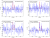 |
Fig. 2 HCN 1-0 spectra towards the comet ER61, E4, V2, and Ol. Scales are as in Fig. 1. |
| In the text | |
|
Fig. 3 CH3OH spectrum towards the comet 96P/Machholz on 30 October 2017. The positions where the CH3OH lines would appear are indicated by the red bars. Scales are as in Fig. 1. |
| In the text | |
|
Fig. 4 Top: HCN 1–0 spectrum towards the comet 46P/Wirtanen on 20 December 2018. The positions, corresponding to a frequency throw of 7 MHz, of the negative artifacts of the HCN lines have been marked with negative dashed red lines. Bottom: global average of all high-resolution (0.1 km s−1) HCN data observed from 20 December 2018 to 18 January 2019. Scales are as in Fig. 1. |
| In the text | |
|
Fig. 5 OSO 20-m HCN 1–0 monitoring data towards 46P/Wirtanen in December 2018 and January 2019. The data points (blue marker with vertical lσ errors bars; horizontal bars indicate the range of observations), which are also listed in Table 4, represent the integrated intensity as a function of MJD or days from perihelion. The dashed lines represent the results from the radiative transfer modelling (see Sect. 4) using three different HCN production rates from 0.5 × 1025mol s−1 to 1.5 × 1025 mol s−1 as indicated for a temperature of 70 K and |
| In the text | |
|
Fig. 6 OSO 20-m methanol spectra towards 46P/Wirtanen when averaging data between 22 and 28 December 2018. The red spectra represent the modelling results of the radiative transfer modelling (see Sect. 4) using a CH3OH production rate of 1.6 × 1026 mol s−1 and a kinetic temperature of 70 K. |
| In the text | |
|
Fig. 7 Top: OSO 20-m HCN 1–0 spectrum towards C/2018 Yl (Iwamoto). It is an average of data between 10 and 19 February 2019. Bottom: HCN spectrum observed towards 2I/Borisov in October/November 2019. Scales are as in Fig. 1. |
| In the text | |
|
Fig. 8 HCN and H20 production rates in 46P/Wirtanen as a function of days from perihelion (12.9 December 2018 UT). The HCN rates (blue) were determined from the intensities (only those detected above the 3σ- level) in Table 4. The water production rates (red) contemporary with our QHCN results, are from Combi et al. (2020). The perihelion value of |
| In the text | |
|
Fig. A.1 Time-dependent HCN modelling with parameters corresponding to the fragment B of 73P/Schwassmann-Wachmann. The upper plot shows the fractional level populations for levels J = 2,3,4 as a function of cometocentric distance. The middle plot shows the relative importance of different downward rates for the HCN J = 3 − 2 transition. As indicated, the included rates are radiative (excluding IR pumping rates), and collisional rates both for electrons and water molecules. The sum of these rates is included as a black line. They are normalized with the time-dependent rate due to destruction and constant expansion; see Eq. (5). The bottom panel depicts the radial density variations. The blue curve is the total HCN density and the green curve represents the water density behaviour. The electron density, ne(r), is drawn in red. Also the HCN/H2O ratio is shown. It is not entirely flat, because when the photodissociation becomes important in the outer coma, HCN and H2O molecules are destroyed with slightly different rates. |
| In the text | |
|
Fig. A.2 HCN level (J = 0 to 5) population variation as a function of cometocentric radius, for the time-dependent modelling (see Fig. A.1) adopting the parameters for fragment B of 73P/Schwassmann-Wachmann during its 2006 passage. The level populations have been normalised to their SE-values to visualise time-dependent effects. The vertical dotted lines correspond to radii RCS and 2RCS between which the electron temperature increases from 90 K to 104 K. |
| In the text | |
Current usage metrics show cumulative count of Article Views (full-text article views including HTML views, PDF and ePub downloads, according to the available data) and Abstracts Views on Vision4Press platform.
Data correspond to usage on the plateform after 2015. The current usage metrics is available 48-96 hours after online publication and is updated daily on week days.
Initial download of the metrics may take a while.