| Issue |
A&A
Volume 660, April 2022
|
|
|---|---|---|
| Article Number | A96 | |
| Number of page(s) | 19 | |
| Section | Stellar structure and evolution | |
| DOI | https://doi.org/10.1051/0004-6361/202142323 | |
| Published online | 20 April 2022 | |
Stable nickel production in type Ia supernovae: A smoking gun for the progenitor mass?
1
Aix Marseille Univ, CNRS, CNES, LAM, Marseille, France
2
Unidad Mixta Internacional Franco-Chilena de Astronomía, CNRS/INSU UMI 3386 and Instituto de Astrofísica, Pontificia Universidad Católica de Chile, Santiago, Chile
e-mail: This email address is being protected from spambots. You need JavaScript enabled to view it.
3
E.T.S. Arquitectura del Vallès, Universitat Politècnica de Catalunya, Carrer Pere Serra 1-15, 08173 Sant Cugat del Vallès, Spain
4
School of Earth and Space Exploration, Arizona State University, Tempe, AZ, USA
5
Joint Institute for Nuclear Astrophysics Center for the Evolution of the Elements, USA
6
Institut d’Astrophysique de Paris, CNRS-Sorbonne Université, 98 bis boulevard Arago, 75014 Paris, France
7
Department of Physics and Astronomy & Pittsburgh Particle Physics, Astrophysics, and Cosmology Center (PITT PACC), University of Pittsburgh, 3941, O’Hara Street, Pittsburgh, PA 15260, USA
Received:
28
September
2021
Accepted:
26
January
2022
Abstract
Context. At present, there are strong indications that white dwarf (WD) stars with masses well below the Chandrasekhar limit (MCh ≈ 1.4 M⊙) contribute a significant fraction of SN Ia progenitors. The relative fraction of stable iron-group elements synthesized in the explosion has been suggested as a possible discriminant between MCh and sub-MCh events. In particular, it is thought that the higher-density ejecta of MCh WDs, which favours the synthesis of stable isotopes of nickel, results in prominent [Ni II] lines in late-time spectra (≳150 d past explosion).
Aims. We study the explosive nucleosynthesis of stable nickel in SNe Ia resulting from MCh and sub-MCh progenitors. We explore the potential for lines of [Ni II] in the optical an near-infrared (at 7378 Å and 1.94 μm) in late-time spectra to serve as a diagnostic of the exploding WD mass.
Methods. We reviewed stable Ni yields across a large variety of published SN Ia models. Using 1D MCh delayed-detonation and sub-MCh detonation models, we studied the synthesis of stable Ni isotopes (in particular, 58Ni) and investigated the formation of [Ni II] lines using non-local thermodynamic equilibrium radiative-transfer simulations with the CMFGEN code.
Results. We confirm that stable Ni production is generally more efficient in MCh explosions at solar metallicity (typically 0.02–0.08 M⊙ for the 58Ni isotope), but we note that the 58Ni yield in sub-MCh events systematically exceeds 0.01 M⊙ for WDs that are more massive than one solar mass. We find that the radiative proton-capture reaction 57Co(p, γ)58Ni is the dominant production mode for 58Ni in both MCh and sub-MCh models, while the α-capture reaction on 54Fe has a negligible impact on the final 58Ni yield. More importantly, we demonstrate that the lack of [Ni II] lines in late-time spectra of sub-MCh events is not always due to an under-abundance of stable Ni; rather, it results from the higher ionization of Ni in the inner ejecta. Conversely, the strong [Ni II] lines predicted in our 1D MCh models are completely suppressed when 56Ni is sufficiently mixed with the innermost layers, which are rich in stable iron-group elements.
Conclusions. [Ni II] lines in late-time SN Ia spectra have a complex dependency on the abundance of stable Ni, which limits their use in distinguishing among MCh and sub-MCh progenitors. However, we argue that a low-luminosity SN Ia displaying strong [Ni II] lines would most likely result from a Chandrasekhar-mass progenitor.
Key words: supernovae: general / nuclear reactions, nucleosynthesis, abundances / supernovae: individual: SN 2017bzc / radiative transfer
© S. Blondin et al. 2022
 Open Access article, published by EDP Sciences, under the terms of the Creative Commons Attribution License (https://creativecommons.org/licenses/by/4.0), which permits unrestricted use, distribution, and reproduction in any medium, provided the original work is properly cited.
1. Introduction
In the long-standing model for type Ia supernovae (SNe Ia), a carbon-oxygen white dwarf (CO WD) star accretes material from a binary companion until it approaches the Chandrasekhar-mass limit for a relativistic degenerate electron plasma (MCh ≈ 1.4 M⊙). While this model provides a robust ignition mechanism for runaway carbon fusion, it is in tension with the observed SN Ia rate (see e.g. Maoz & Mannucci 2012; Livio & Mazzali 2018; Wang 2018; Soker 2019 for reviews). Moreover, there is growing evidence that it cannot explain the full range of observed SN Ia properties (e.g. Jha et al. 2019). For instance, Flörs et al. (2020) find that the Ni/Fe abundance ratio inferred from late-time spectroscopy is consistent with the predictions of sub-MCh models for 85% of normal SNe Ia.
There are multiple paths leading to the explosion of a WD significantly below the Chandrasekhar-mass limit. In double-detonation models (e.g. Shen et al. 2018; Townsley et al. 2019; Magee et al. 2021; Gronow et al. 2021), a sub-MCh WD accretes a thin He-rich layer from a non-degenerate binary companion, triggering a detonation at its base which leads to a secondary detonation of the CO core. Modern incarnations of this model consider modestly CO-enriched low-mass He layers (≲10−2 M⊙), whose detonation does not lead to spurious spectroscopic features from iron-group elements (IGEs) at early times (Shen & Moore 2014; Townsley et al. 2019). Furthermore, the predicted rate of double-detonation models matches the observed SN Ia rate (e.g. Ruiter et al. 2011, 2014).
Other sub-MCh progenitor models involve double-WD systems. In the classical double-degenerate model of Webbink (1984), two unequal-mass WDs in a close binary system merge through loss of energy and angular momentum via gravitational-wave radiation. The more massive WD tidally disrupts and accretes the lower-mass object, resulting in an off-centre carbon ignition in the merger remnant and the formation of an oxygen-neon (ONe) WD (e.g. Saio & Nomoto 1985; Timmes et al. 1994; Shen et al. 2012). If the remnant mass exceeds the Chandrasekhar limit, accretion-induced collapse to a neutron star ensues, associated with a weak explosion, but with no SN Ia event (Nomoto & Kondo 1991).
This model was later revised by Pakmor et al. (2010), who considered the merger of two nearly equal-mass WDs, in which the less massive WD is rapidly accreted onto the primary WD, resulting in compressional heating of the accreted material and subsequent carbon ignition. Such violent merger models have been successful in reproducing the observed properties of both sub-luminous and normal SNe Ia (Pakmor et al. 2010, 2012), as well as more peculiar events (Kromer et al. 2013, 2016).
In addition to mergers, several authors have explored collisions between two WDs as a potential SN Ia progenitor scenario (e.g. Raskin et al. 2009; Rosswog et al. 2009). Such collisions are expected to occur in dense stellar environments such as globular clusters (e.g. Hut & Inagaki 1985; Sigurdsson & Phinney 1993); it was more recently suggested that they may efficiently occur in triple systems to explain SNe Ia (Katz & Dong 2012; Kushnir et al. 2013), although the predicted rates vary significantly (see e.g. Toonen et al. 2018). Furthermore, Dong et al. (2015) argued that the doubly peaked line profiles observed in late-time spectra of several SNe Ia result from a bimodal 56Ni distribution produced in WD–WD collisions.
It should be possible to identify SNe Ia resulting from MCh vs. sub-MCh progenitors observationally, since variations in the ejecta mass have an impact on the radiative display (e.g. Pinto & Eastman 2000). The typical photon diffusion time depends on the mean opacity, κ, of the ejecta, its mass, Mej, and characteristic velocity, v, following  (e.g. Arnett 1982; Woosley et al. 2007; Piro et al. 2010; Khatami & Kasen 2019). The photon diffusion time is thus shorter for a sub-MCh ejecta compared to a MCh ejecta, resulting in shorter bolometric rise times (see e.g. Blondin et al. 2017). The post-maximum bolometric decline is also faster, as the lower density of sub-MCh ejecta favours the earlier escape of γ-rays (e.g. Kushnir et al. 2020; Sharon & Kushnir 2020)1.
The colour evolution around maximum light is also affected by the ejecta mass. As noted by Blondin et al. (2017), sub-MCh ejecta are subject to a larger specific heating rate at maximum light2 for a given 56Ni mass, owing to the shorter rise times and lower ejecta mass; hence, they display bluer maximum-light colours. The colour evolution past maximum light is also more pronounced, as observed in low-luminosity SNe Ia (e.g. Blondin et al. 2017; Shen et al. 2021). The ejecta mass can, in principle, be constrained based purely on photometric indicators. In practice, however, their interpretation is subject to uncertainties in the radiative-transfer modelling (see e.g. discussion in Blondin et al. 2018).
A more robust signature of the WD mass should therefore be sought in the spectroscopic signatures of distinct abundance patterns predicted by different explosion models; in particular, the density at which the CO fuel is ignited affects the resulting nucleosynthesis. More specifically, Chandrasekhar-mass WDs have central densities ρc ≳ 109 g cm−3, where explosion models involving sub-MCh WDs (including WD mergers and collisions) detonate the CO core in regions with ρ ≲ 108 g cm−3. The higher densities in MCh models result in a higher electron-capture rate during the explosion, which enhances the production of neutron-rich stable isotopes of iron-group elements compared to sub-MCh models.
Of particular interest are the stable isotopes of nickel, the most abundant of which is 58Ni. At sufficiently late times (≳150 d past explosion), SN Ia spectra are dominated by forbidden lines of singly and doubly ionized Ni, Co, and Fe. By then, the only nickel left in the ejecta is stable Ni synthesized in the explosion, whereas most of the Co is 56Co from 56Ni decay, and Fe is a mixture of primordial stable Fe and 56Fe from 56Ni decay. The larger abundance of stable Ni in MCh models is thus expected to manifest itself in the form of forbidden lines of [Ni II], which have been detected in late-time spectra of several SNe Ia to date (e.g. Dhawan et al. 2018; Maguire et al. 2018; Flörs et al. 2018, 2020). These lines ought to be largely suppressed if not completely absent from sub-MCh models due to the lower abundance of stable Ni.
In principle, we thus have a clear prediction in terms of stable Ni production that depends on the mass of the exploding WD and an associated spectroscopic diagnostic to distinguish between MCh and sub-MCh models. This was partly confirmed by Blondin et al. (2018) for low-luminosity SN Ia models: the MCh model displayed a prominent line due to [Ni II] 1.94 μm, where the sub-MCh model showed no such line.
In this paper, we test whether this prediction holds for higher-luminosity models, which correspond to the bulk of the SN Ia population, and to what extent the abundance of stable Ni is the determining factor in explaining the strength of [Ni II] lines in late-time SN Ia spectra. We first briefly present the SN Ia models and numerical methods in Sect. 2. We investigate the dominant nuclear reactions responsible for stable Ni production and present a census of 58Ni yields in MCh versus sub-MCh models in Sect. 3. We discuss the relative impact of Ni abundance and ionization on nebular [Ni II] lines in Sect. 4, as well as the impact of mixing in Sect. 5. Our conclusions follow in Sect. 6.
2. Explosion models and radiative transfer
We base our analysis on previously published SN Ia explosion models. One exception is the 1D MCh delayed-detonation model 5p0_Z0p014, published here for the first time, whose WD progenitor results from the evolution of a 5 M⊙ star at solar metallicity (Z = 0.014; Asplund et al. 2009). The explosive phase was simulated using the same hydrodynamics and nucleosynthesis code as the sub-MCh detonation models 1p06_Z2p25e-2 and 0p88_Z2p25e-2 from a 1.06 M⊙ and 0.88 M⊙ WD progenitor, respectively, at slightly super-solar metallicity (Z = 0.025 ≈ 1.6 Z⊙; Bravo et al. 2019). Basic model properties and various nickel isotopic abundances are given in Table A.1.
The synthetic late-time spectra (∼190 d past explosion) presented in Sects. 4 and 5 were computed using the 1D, time-dependent, non-local thermodynamic equilibrium radiative-transfer code CMFGEN of Hillier & Dessart (2012). Late-time spectra for the low-luminosity MCh delayed-detonation model DDC25 and the sub-MCh detonation model SCH2p0 are from Blondin et al. (2018). Those for the high-luminosity MCh delayed-detonation model DDC0 and the sub-MCh detonation model SCH7p0 are published here for the first time. The same is true of the mixed versions of the MCh delayed-detonation model DDC15 (Sect. 5). All model outputs are publicly available online3.
3. Stable Ni production in MCh vs. sub-MCh models
3.1. Nuclear statistical equilibrium
Explosive burning at sufficiently high temperatures (T ≳ 5 × 10⁹ K) results in a state of balance between forward and reverse nuclear reactions known as nuclear statistical equilibrium (NSE; see e.g. Clifford & Tayler 1965; Woosley et al. 1973; Hartmann et al. 1985; Cabezón et al. 2004; Nadyozhin & Yudin 2004). Such temperatures are reached in the inner layers of both MCh delayed-detonation models and sub-MCh detonation models, although the highest temperatures ≲1010 K are only reached in MCh models (Fig. 1). In NSE, the yields do not depend on the initial composition but are instead uniquely determined by the peak temperature (Tpeak), the density at Tpeak (ρpeak), and the electron fraction, Ye = ∑i(Zi/Ai)Xi, where Xi is the mass fraction of a particular isotope i with atomic number Zi and mass number Ai.
 |
Fig. 1. Density at peak temperature (ρpeak) versus peak temperature (Tpeak, in units of 109 K) in the MCh delayed-detonation model 5p0_Z0p014 (filled circles) and the sub-MCh detonation models 1p06_Z2p25e-2 (MWD = 1.06 M⊙, filled squares) and 0p88_Z2p25e-2 (MWD = 0.88 M⊙, filled triangles). The wide vertical band denotes the transition between incomplete Si burning and complete burning to NSE. The NSE region is further subdivided into ‘normal’ and ‘alpha-rich’ freeze-out regimes. The width of the bands correspond to variations in the post-burn cooling time scale (Woosley et al. 1973; see also Lach et al. 2020, their Fig. 1). |
The electron fraction of the WD prior to explosion is set by the metallicity of the progenitor star on the main sequence, which is routinely parametrized by adjusting the abundance of the neutron-rich isotope 22Ne. Here, the assumption is that the CNO catalysts all end up as 14N at the end of the hydrogen-burning phase, which is then converted to 22Ne via 14N(α,γ)18F(β+,νe)18O(α,γ)22Ne during the helium-core burning phase (see Timmes et al. 2003), such that:
![Mathematical equation: $$ \begin{aligned} X(^{22}\mathrm{Ne} ) = 22 \left[ \frac{X(^{12}\mathrm{C} )}{12} + \frac{X(^{14}\mathrm{N} )}{14} + \frac{X(^{16}\mathrm{O} )}{16} \right] \approx 0.013 \left(\frac{Z}{\mathrm{Z} _\odot }\right), \end{aligned} $$](/articles/aa/full_html/2022/04/aa42323-21/aa42323-21-eq2.gif) (1)
(1)
where we used the solar CNO abundances from Asplund et al. (2009) and isotopic ratios from Lodders (2003) 4. We ignore the initial 22Ne of the progenitor star as its mass fraction is ∼10−4 at solar metallicity.
In addition to 22Ne resulting from the CNO cycle, the initial metallicity is also determined by the abundance of 56Fe nuclei inherited from the ambient interstellar medium. For a WD composed of only 12C, 16O, 22Ne, and 56Fe (i.e. X(12C)+X(16O)=1 − X(22Ne)−X(56Fe)), the electron fraction is (see also Kushnir et al. 2020):
 (2)
(2)
where we have used the solar Fe abundance X(Fe)=1.292 × 10⁻³ from Asplund et al. (2009) and the 56Fe isotopic fraction of 91.754% from Lodders (2003), yielding X(56Fe) ≈ 1.185 × 10⁻³(Z/Z⊙). In this framework, a solar-metallicity WD has X(22Ne)≈0.0135 and Ye ≈ 0.49935. A larger metallicity corresponds to a larger 22Ne abundance and in turn a lower Ye.
In MCh models this baseline Ye can, in principle, be reduced via weak reactions on carbon during the convective burning (or ‘simmering’) phase prior to thermonuclear runaway (e.g. Piro & Bildsten 2008; Chamulak et al. 2008; Schwab et al. 2017), although Martínez-Rodríguez et al. (2016) show the impact to be negligible (reduction in Ye of ≲10−4 ; but see Piersanti et al. 2017 for a different view). However, the higher densities of MCh WDs (up to 2−3 × 10⁹ g cm−3; see Fig. 1) result in a significant electron-capture rate during the initial deflagration phase of delayed-detonation models. This lowers the Ye far below the baseline value (Fig. 2, top panel) and favours the synthesis of neutron-rich isotopes in the innermost layers (v ≲ 3000 km s−1; Fig. 2, middle panel). For nickel, this results in the synthesis of the stable isotopes 58Ni, 60Ni, 61Ni, 62Ni, and 64Ni instead of the radioactive 56Ni (for which Ye = 0.5).
 |
Fig. 2. Top panel: electron fraction profile at t ≈ 30 min past explosion in the inner ejecta of the MCh delayed-detonation model 5p0_Z0p014 (dashed line) and the MWD = 1.06 M⊙ sub-MCh detonation model 1p06_Z2p25e-2 (solid line) shown in Fig. 1. The markers in the upper panel are shown such that the ordinate corresponds to the Ye of the nucleus (e.g. Ye = 28/58 ≈ 0.483 for 58Ni) and the abscissa to the interpolated velocity on the Ye profile for the MCh delayed-detonation model (both 56Ni and 64Ni are synthesized in this model but the Ye profile does not intersect the Ye value of either isotope). Middle and bottom panels: abundance profiles of stable Ni isotopes for both models. The insets correspond to a logarithmic scale, revealing minor contributions to the total stable Ni abundance from 61Ni for the MCh model and from both 61Ni and 62Ni for the sub-MCh model. No 64Ni is produced in this sub-MCh model. |
In detonations of sub-MCh WDs, however, the burning timescale is much shorter than the weak-reaction timescale, such that Ye remains constant at its baseline value (Ye ≈ 0.49935 for a solar-metallicity WD) throughout the burning phase. Stable neutron-rich isotopes of nickel are still synthesized in NSE at this Ye at the peak temperatures (5 − 6 × 10⁹ K) and densities (107 − 108 g cm−3), characteristic of the inner ejecta of sub-MCh detonations (Fig. 2, bottom panel). These conditions are similar to those encountered in the layers of MCh models where most of the 58Ni is synthesized (v ≈ 2000 km s−1 for the MCh model shown in Fig. 2). By comparing the NSE distributions for Ye = 0.499 and Ye = 0.48 in Fig. 3 (top panel), we see that the 58Ni abundance in sub-MCh detonations can be comparable to (and even exceed) that of MCh delayed-detonation models, with predicted mass fractions X(58Ni) ≈ 0.1.
3.2. Freeze-out yields
The final isotopic abundances can differ significantly from their NSE value during the so-called freeze-out phase, when free particles (protons, neutrons, α particles) reassemble into nuclei on a timescale of  (e.g. Magkotsios et al. 2010). For high densities (≳108 − 109 g cm−3), this timescale is short and for T ≲ 7 × 10⁹ K the α abundance is low (normal freeze-out), such that the final abundances do not differ greatly from their NSE value. However, for the lower ρpeak relevant to the synthesis of 58Ni (107 − 108 g cm−3), the freeze-out timescale is longer and the α abundance is higher (X(4He)≈0.1; alpha-rich freeze-out), and the final yields of stable Ni isotopes can differ significantly from their NSE values (Fig. 3, bottom panel).
 |
Fig. 3. Top panel: NSE distributions for 58Ni as a function of temperature (in units of 109 K) for Ye = 0.48 (dashed lines) and Ye = 0.499 (solid lines), at densities of 107 g cm−3 (thin lines) and 108 g cm−3 (thick lines). These NSE distributions were computed with the public_nse code (Publicly available on F. X. Timmes’ webpage; http://cococubed.asu.edu/code_pages/nse.shtml) (see also Seitenzahl et al. 2008). Bottom panel: freeze-out yields based on the adiabatic thermodynamic trajectories of Magkotsios et al. (2010) for the same set of (ρpeak, Ye) values. |
In either case, the freeze-out timescale is significantly shorter than the weak-reaction timescale, such that Ye remains roughly constant during the freeze-out. Stable isotopes of Ni are synthesized preferentially in shells with a similar Ye value. This is illustrated by the MCh delayed-detonation model in the bottom panel of Fig. 2, where the peak in the stable Ni abundance profile at ∼2000 km s−1 consists almost exclusively of the 58Ni isotope (see inset). The Ye of this isotope (Ye = 28/58 ≈ 0.48) coincides with the Ye value at this velocity coordinate (Fig. 2, top panel), where the peak temperature is ∼5 × 10⁹ K and the density 2 − 3 × 10⁷ g cm−3. Under these conditions, the predicted freeze-out mass fraction for 58Ni is a few times 0.1 (Fig. 3, bottom panel), which is on par with the MCh model yield. The more neutron-rich isotopes 60Ni, 61Ni, 62Ni, and 64Ni are synthesized at lower velocities ≲1500 km s−1, where the density is higher – and hence the Ye value is lower as a result of electron captures.
For the sub-MCh detonation model, the stable Ni mass fraction remain roughly constant at 5 − 6 × 10⁻² throughout the inner ejecta. These mass fractions are in agreement with the predicted freeze-out 58Ni yields for Ye = 0.499 and densities in the range 107 − 108 g cm−3 for peak temperatures 5 − 6 × 10⁹ K (Fig. 3, bottom panel). In MCh models, 58Ni is synthesized in layers with similar (Tpeak, ρpeak) conditions, but at a lower Ye ≈ 0.48, which results in an order-of-magnitude difference in the predicted freeze-out yields.
3.3. Decayed yields at one year past explosion
Once the burning phase has ceased (typically a few seconds after the beginning of the thermonuclear runaway), the stable Ni yield continues to increase through radioactive decays with half-lives trac12 ≳ 1 s, in particular via the β+ decay chains 60, 61, 62Zn →60, 61, 62Cu →60, 61, 62Ni (see Table 1). From this point, we go on to consider the decayed yields at one year past explosion when referring to the 58Ni or stable Ni yields, as these are most relevant to the late-time spectra discussed in this paper. We note, however, that the decayed 58Ni yield is set shortly after explosion, since the only parent isotope, 58Cu, decays to 58Ni with a half-life of ∼3.2 s.
Radioactive decay chains with half-lives trac12 > 1 s ending in a stable isotope of nickel.
3.4. Synthesis of the stable isotope 58Ni
For all the models studied here with a 58Ni yield larger than 0.01 M⊙, more than 60% of all the stable Ni is in the form of 58Ni (see Table A.1)6. This fraction rises above 80% for models with a 58Ni yield larger than 0.04 M⊙. For comparison, the isotopic fraction of 58Ni on Earth and in the Sun is ∼68% (Lodders 2003). In both the MCh delayed-detonation model 5p0_Z0p014 and the sub-MCh detonation model 1p06_Z2p25e-2 (described in the previous section), this isotope is mainly synthesized through the reactions depicted in Fig. 4, where the reaction probabilities correspond to the aforementioned sub-MCh model. They were obtained by integrating the net reaction fluxes (mol g−1) and calculating the relative contributions of each reaction to the total net flux. Thus, in this model, 57Cu is synthesized 81.5% of the time via 56Ni(p, γ) and the remaining 18.5% via 60Zn(p, α). The probabilities do not always add up to 100%, as other more minor reactions can contribute to a specific isotope. Most notably 58Ni is also synthesized via 58Co(p, n) (6.13%), 61Cu(p, α) (4.85%), 55Fe(α, n) (2.26%), 54Fe(α, γ) (2.04%), 57Ni(n, γ) (1.25%), 58Cu(n, p) (0.51%), 62Zn(γ, α) (0.38%), and 61Zn(n, α) (0.01%), in addition to the two dominant reactions 57Co(p, γ) (69.5%) and 59Ni(γ, n) (13.0%).
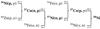 |
Fig. 4. Main reactions resulting in the synthesis of stable 58Ni. The numbers give the probability for a given reaction product to result from a specific reactant in the sub-MCh model 1p06_Z2p25e-2 (see text for details). |
The dominant reaction chain is highlighted in bold: 56Ni(p,γ)57Cu(n,p)57Ni(n,p)57Co(p,γ)58Ni. The probability for a 58Ni nucleus to result from a particular reactant nucleus is simply obtained by multiplying the reaction probabilities along the chain. Thus 0.815 × 0.643 × 0.418 × 0.695 ≈ 0.152 or 15.2% of 58Ni nuclei result from the reaction chain starting with 56Ni in this model. The majority of 56Ni does not end up as 58Ni, of course, as many 56Ni nuclei survive the explosive phase to later decay radioactively via the 56Ni→56Co→56Fe chain and power the SN Ia light curve.
Among all reactions ending in 58Ni, the final 58Ni abundance is mostly determined by the rate for the radiative proton-capture reaction 57Co(p, γ)58Ni. This might appear surprising since an α-rich freeze-out from NSE should favour α captures on 54Fe as the main production route for 58Ni, in particular 54Fe(α, γ)58Ni. However, this reaction only contributes ∼2% of the net nucleosynthetic flux to 58Ni in this model. In spite of the seemingly large contribution of 54Fe(α, p) to the synthesis of 57Co (34.5%) and of 54Fe(α, n) to that of 57Ni (55.6%), artificially inhibiting all α captures (with either γ, neutron or proton output channels) on 54Fe has a negligible impact on the final 58Ni abundance compared to when the radiative proton-capture reaction 57Co(p, γ)58Ni is artificially switched off.
Nonetheless, the preferred reaction chain from 54Fe to 58Ni during freeze-out mimics the α-capture reaction 54Fe(α, γ)58Ni, as it proceeds first via two radiative proton captures to 56Ni, namely, 54Fe(p,γ)55Co(p,γ)56Ni, followed by the reaction chain outlined in bold above from 56Ni to 58Ni. The entire process then consists of four (p,γ) and two (n,p) reactions, which is indeed equivalent to the net capture of an α particle (2n + 2p). While the abundance of α particles is large in α-rich freeze-out by definition, the abundance of free neutrons and protons is even more enhanced compared to that in a normal freeze-out.
Although the 57Co(p, γ)58Ni reaction dominates the reaction chain ending in 58Ni, the synthesis of this isotope in Chandrasekhar-mass WDs is mostly affected by the amount of electron captures in NSE. Since 56Ni is the most abundant isotope when NSE is achieved at the neutron excess inherited from the progenitor (see Fig. 2), the yield of 58Ni is most sensitive to the electron-capture rate on 56Ni and, to a lesser extent, on 55Co. However, the yield of 58Ni is quite robust as it changes by ∼20% for a two orders-of-magnitude change in any electron-capture rate (see Bravo 2019 for more details).
3.5. 58Ni yields in MCh and sub-MCh models
We show the decayed 58Ni yield at t = 1 yr past explosion as a function of the 56Ni mass at t ≈ 0 for a variety of SN Ia explosion models in Fig. 5. In the following subsections, we first discuss MCh models and then sub-MCh models. We include violent WD mergers and WD collisions in sub-MCh models since the mass of the exploding WD is below MCh, despite the combined mass of both WDs sometimes exceeding this value.
 |
Fig. 5. Stable 58Ni yield at t = 1 yr past explosion versus radioactive 56Ni yield at t ≈ 0 for various SN Ia explosion models (MCh models in red, sub-MCh models in blue). Chandrasekhar-mass models include: deflagrations (3D models of Fink et al. 2014; 1D W7 model of Mori et al. 2018), delayed detonations (3D models of Seitenzahl et al. 2013; 2D models of Kobayashi et al. 2020; 1D models of Blondin et al. 2013; 1D model 5p0_Z0p014 from this paper), and gravitationally confined detonations (3D model of Seitenzahl et al. 2016). Sub-MCh models include: detonations (1D models of Blondin et al. 2017; 1D 1 M⊙ models of Shen et al. 2018; 1D models of Bravo et al. 2019; 1D models of Sim et al. 2010; 1D models of Kushnir et al. 2020), double detonations (3D models of Gronow et al. 2021; 2D models of Kobayashi et al. 2020; 2D model of Townsley et al. 2019), detonations in ONe WDs (2D models of Marquardt et al. 2015), violent WD mergers (3D models of Pakmor et al. 2011, 2012 and Kromer et al. 2013, 2016), and WD–WD collisions (2D models of Kushnir 2021, priv. comm.). |
3.5.1. Chandrasekhar-mass models
Deflagrations. Laminar flames in SNe Ia quickly become turbulent as buoyant hot ashes rise through overlying cold fuel, generating Rayleigh–Taylor and Kelvin–Helmholtz instabilities that increase the flame surface and hence the rate of fuel consumption. Deflagrations are thus best studied in 3D, and we base our discussion on the models of Fink et al. (2014) 7. Since the precise initial conditions at the onset of thermonuclear runaway remain unknown to a large extent, the deflagration is artificially ignited in a number Nk of spherical ignition spots (or ‘kernels’) simultaneously. In their study, Fink et al. (2014) consider Nk = 1, 3, 5, 10, 20, 40, 100, 150, 200, 300, and 1600 such kernels distributed at random around the WD centre.
As Nk increases, the rate of fuel consumption (and hence nuclear energy release) also increases, resulting in a more rapid flame growth and more material being burnt. Thus, increasing Nk results in a higher production of both stable 58Ni and radioactive 56Ni, which explains the monotonic sequence in Fig. 5 (open squares) up until Nk = 150. For higher Nk, the nuclear energy release is so high early on that the resulting WD expansion quenches nuclear reactions, resulting in less material being burnt. Thus, while the 58Ni yield continues to increase with Nk (as this stable isotope is mainly produced during the initial stages of the deflagration), the 56Ni yield remains more or less constant, even decreasing slightly for Nk = 1600 (model N1600def).
The models of Fink et al. (2014) enable us to study the impact of variations in the central density of the progenitor WD for model N100def (dashed line in Fig. 5). A lower central density of ρc = 1.0 × 10⁹ g cm−3 results in a ∼50% lower 58Ni yield owing to the lower electron-capture rate during the initial deflagration. However, increasing ρc to 5.5 × 10⁹ g cm−3 results in a similar 58Ni yield as in the base model with ρc = 2.9 × 10⁹ g cm−3, but the yield of heavier stable Ni isotopes more than doubles (see Table A.1).
For completeness we show the widely used 1D deflagration model W7 of Nomoto et al. (1984) as computed by Mori et al. (2018) with updated electron-capture rates. In this model, the deflagration front is artificially accelerated from 8 to 30% of the local sound speed. The initial propagation of the deflagration flame results in a similar electron-capture rate compared to the most energetic 3D deflagration models of Fink et al. (2014), with a 58Ni yield of ∼0.07 M⊙. However the gradual acceleration of the flame results in a more complete burn of the outer layers and a larger 56Ni yield compared to standard deflagration models. Leung & Nomoto (2018) find similar 56Ni and stable Ni yields but they also consider W7 models at sub-solar metallicities (0.1 and 0.5 Z⊙). Interestingly, the impact on the stable Ni yield is negligible (≲4%; see Table A.1).
Delayed detonations. In the 1D delayed-detonation models shown here (DDC series of Blondin et al. 2013), the 58Ni yield is relatively constant at ∼0.025 M⊙ regardless of the 56Ni mass. Stable Ni isotopes are almost exclusively synthesized in high-density burning conditions during the early deflagration phase, with almost no stable Ni produced during the subsequent detonation phase (where most of the radioactive 56Ni is synthesized). The exception is model DDC0 which has the largest 56Ni yield (0.84 M⊙) for which an additional ∼0.01 M⊙ of 58Ni is synthesized during the detonation phase at expansion velocities 5000 − 8500 km s−1 (corresponding to mass coordinates ∼0.3 − 0.65 M⊙), where the peak temperatures reach 5.5−6.9 × 10⁹ K at densities 2.5−5.8 × 10⁷ g cm−3.
The situation is somewhat different in 3D simulations where a substantial amount of stable Ni is synthesized during the detonation phase. The weaker the initial deflagration (i.e. the lower the number of ignition kernels), the smaller the WD pre-expansion prior to the deflagration-to-detonation transition and the higher the burning density during the detonation phase. As a result, more stable IGEs (as well as radioactive 56Ni) are synthesized during the detonation. An extreme example is model N1 (only one ignition kernel ignites the initial deflagration), which synthesizes more than 0.07 M⊙ of 58Ni and more than 1.1 M⊙ of 56Ni, but whose deflagration counterpart (N1def) synthesizes less than 0.01 M⊙ of 58Ni and less than 0.1 M⊙ of 56Ni. Conversely, one can deduce from comparing models N1600 and N1600def that almost all the stable 58Ni and radioactive 56Ni are synthesized during the deflagration phase, owing to the high number of ignition kernels.
Also shown in Fig. 5 is the impact of varying the central density of the progenitor WD for model N100 (dashed line; see also the 2D models of Kobayashi et al. 2020). As for the deflagration model N100def, a lower central density of ρc = 1.0 × 10⁹ g cm−3 results in a lower 58Ni yield owing to the lower electron-capture rate during the initial deflagration. However, whereas increasing ρc had a negligible impact on the production of stable 58Ni for the deflagration model N100def, the 58Ni yield increases by ∼9% in the delayed-detonation model N100 owing to pockets of high-density fuel burnt during the subsequent detonation phase.
Finally, the impact of decreasing the metallicity of the progenitor WD to one half, one tenth, and one hundredth solar is shown for model N100 (dotted line). As expected, decreasing the metallicity (and hence increasing Ye) favours the synthesis of radioactive 56Ni at the expense of stable 58Ni (see e.g. Timmes et al. 2003).
Kobayashi et al. (2020) recomputed the 2D delayed-detonation models of Leung & Nomoto (2018) by assuming a solar-scaled initial composition as a proxy for the progenitor metallicity. In Fig. 5, we show their Z = 0.02 models for three different central densities corresponding to WD masses of 1.33, 1.37, and 1.38 M⊙ (from low to high 58Ni yield; right half-filled circles connected with a dashed line and labelled ‘zscl’ in Table A.1). As noted in Sect. 3.1, this results in a much lower 22Ne mass fraction at a given metallicity compared to what is expected from the conversion of CNO into 22Ne. This largely explains the lower 58Ni yields compared to the models of Seitenzahl et al. (2013). Kobayashi et al. (2020) also present the original models of Leung & Nomoto (2018) in which the 22Ne mass fraction was set to the progenitor metallicity (labelled ‘zne22’ in Table A.1). In Fig. 5, we show their 1.33 M⊙ and 1.38 M⊙ models at Z = X(22Ne)=0.02. The 58Ni yield is larger by up to a factor of three compared to the corresponding solar-scaled initial composition models (connected via a dotted line). We present models from Kobayashi et al. (2020) at different metallicities in Table A.1.
Gravitationally confined detonation (GCD). In this model, originally proposed by Plewa et al. (2004), burning is initiated as a weak central deflagration which drives a buoyant bubble of hot ash that breaks out at the stellar surface, causing a lateral acceleration and convergence of the flow of material at the opposite end. Provided the density of the compressed material is high enough, a detonation is triggered which incinerates the remainder of the WD.
In Fig. 5, we show the 3D GCD model of Seitenzahl et al. (2016) (half-filled pentagon), with a 58Ni yield of 0.037 M⊙ for a 56Ni yield of 0.742 M⊙. The weak initial deflagration results in little WD pre-expansion. In this respect, it is similar to the delayed-detonation models of Seitenzahl et al. (2013) with a low number of ignition spots, where a significant amount of stable IGEs and 56Ni are synthesized during the detonation phase. However, the WD does expand during the flow convergence phase, so less 58Ni is synthesized compared to delayed-detonation models with similar 56Ni yield.
3.5.2. Sub-Chandrasekhar-mass models
Detonations. For detonations of sub-MCh WDs the main parameter that determines the final yields is the mass of the exploding WD. The propagation of the detonation front is so fast compared to the WD expansion timescale that the density at which material is burnt is close to the original density profile of the progenitor WD. Lower-mass WDs have lower densities at a given mass (or radial) coordinate, so the detonation produces less electron-capture isotopes than for more massive WDs. For the 1D sub-MCh models at solar metallicity shown here (SCH series of Blondin et al. 2017; filled diamonds in Fig. 5), only the highest-mass WDs (MWD > 1.1 M⊙) have a 58Ni yield comparable to 1D delayed-detonation models (DDC series of Blondin et al. 2013). For WD masses below 1 M⊙, the 58Ni yield is significantly lower (< 0.025 M⊙) yet not vanishingly small. Stable 58Ni is still synthesized in detonations of ≲0.90 M⊙ WDs that result in low-luminosity SNe Ia (e.g. Blondin et al. 2018).
Varying the initial metallicity has the same effect as for the MCh delayed-detonation models discussed above. In the 1 M⊙ models of Shen et al. (2018), increasing the metallicity from solar to twice solar results in a factor of ∼2 increase in the 58Ni yield (from 7.05 × 10⁻³ M⊙ to 1.66 × 10⁻² M⊙), whereas decreasing the metallicity from solar to one-half solar results in a factor of ∼3 decrease in the 58Ni yield (from 7.05 × 10⁻³ M⊙ to 2.48 × 10⁻³ M⊙). Similar trends are observed for the slightly super-solar (∼1.6 Z⊙) 1.06 M⊙ model of Bravo et al. (2019) and in the extensive set of 1D sub-MCh models published by Kushnir et al. (2020) 8. We note that 58Ni is still synthesized at zero metallicity in these models (with a yield ∼10−3 M⊙; see Table A.1).
Several sub-MCh models at super-solar metallicities have higher 58Ni (and total stable Ni) yields compared to some of the delayed-detonation models shown here, such as the 3 Z⊙ 1.06 M⊙ model of Sim et al. (2010) 9 and the 2 Z⊙ 1.1 M⊙ model of Kushnir et al. (2020), which yield ∼0.05 M⊙ and ∼0.04 M⊙ of 58Ni, respectively.
Double detonations. These models include a thin accreted helium layer which serves as a trigger for detonating the underlying CO core. Since the nucleosynthesis of 58Ni largely occurs in the CO core, its abundance is expected to be similar to detonations of sub-MCh WDs for a given WD mass. For instance, the 2D double-detonation model of Townsley et al. (2019) from a 1 M⊙ WD progenitor with a 0.021 M⊙ He shell has very similar 56Ni and 58Ni yields compared to the 1 M⊙ solar-metallicity model of Shen et al. (2018). The 3D models of Gronow et al. (2021) display a quasi-linear trend of increasing 58Ni yield with increasing 56Ni mass (and hence progenitor WD mass), with a slight offset to higher 58Ni yields compared to the 1D models of Blondin et al. (2017). For clarity we do not show the zero-metallicity models of Gronow et al. (2020) based on 1.05 M⊙ progenitors as they produce a cluster of points around M(56Ni) ≈ 0.6 M⊙ and M(58Ni) ≈ 10−3 M⊙, although we do include them in Table A.1. We do not show results from the 2D double-detonation models of Fink et al. (2010) as the corresponding abundance data is not available (Röpke 2020, priv. comm.).
Owing to their prescription for the progenitor metallicity (see Sect. 3.1), the 2D double-detonation models of Kobayashi et al. (2020) with solar-scaled initial composition for Z = 0.02 (left half-filled circles in Fig. 5 and labelled ‘zscl’ in Table A.1) have 58Ni yields of a few 10−3 M⊙ at most, comparable to zero-metallicity sub-MCh models published by other groups (e.g. Sim et al. 2010; Kushnir et al. 2020; Gronow et al. 2020). We also show their 1 M⊙ model at Z = 0.02 in which the 22Ne mass fraction was set to the initial metallicity (i.e. X(22Ne)=0.02, labelled ‘zne22’ in Table A.1). The 58Ni yield is one order of magnitude larger compared to the corresponding solar-scaled initial composition model (connected via a dotted line), and the total stable Ni yield is larger by a factor of ∼3.
Detonations in ONe WDs. In the 2D simulations carried out by Marquardt et al. (2015) the progenitor ONe WDs are in the mass range 1.18 − 1.25 M⊙ with corresponding central densities 1.0 − 2.0 × 10⁸ g cm−3, which results in the production of copious amounts of 56Ni (> 0.8 M⊙). The initial composition includes 20Ne but no 22Ne, hence, the 58Ni yield is low (< 5 × 10⁻³ M⊙), comparable to other zero-metallicity models shown in Fig. 5.
Violent WD mergers. In the violent merger of two sub-MCh WDs, the nucleosynthesis of IGEs occurs in similar conditions compared to detonations of single sub-MCh WDs. The secondary (accreted) WD is almost entirely burned in the process but at significantly lower densities, producing intermediate-mass elements from incomplete silicon burning and oxygen from carbon burning, while leaving some unburnt CO fuel. Of the four violent merger models with published nucleosynthesis data, solely the model of Pakmor et al. (2012) corresponding to the violent merger of two CO WDs of 0.9 M⊙ and 1.1 M⊙ has a significant 58Ni yield (∼0.028 M⊙). The other three models have either overly low metallicity (0.9 + 0.9 M⊙ model of Pakmor et al. 2011 at zero metallicity; 0.9 + 0.76 M⊙ model of Kromer et al. 2016 at Z = 0.01; both yield a few times 10−5 M⊙ of 58Ni) or reach too low a peak density during the detonation (ρpeak ≲ 2 × 10⁶ g cm−3 in the 0.9 + 0.76 M⊙ model of Kromer et al. 2013; the 58Ni yield is ∼0.002 M⊙).
WD–WD collisions. Following the pioneering work of Benz et al. (1989), several groups have performed 3D simulations of WD collisions with varying mass ratios and impact parameters (Raskin et al. 2009, 2010; Rosswog et al. 2009; Lorén-Aguilar et al. 2010; Hawley et al. 2012). However, all of these studies consider pure CO WDs (i.e. no 22Ne, equivalent to zero metallicity in our framework), and none report 58Ni yields due to their use of limited nuclear reaction networks (the yield is expected to be low due to the zero metallicity, as in the 2D simulations of Papish & Perets 2016 who report 58Ni yields ≲0.005 M⊙ for two of their models).
Here, we show the preliminary results of 2D simulations by Kushnir (2021, priv. comm.) consisting of equal-mass WD–WD collisions. From low to high 56Ni yield, the WD masses are: 0.5–0.5 M⊙, 0.6–0.6 M⊙, 0.7–0.7 M⊙, 0.8–0.8 M⊙, 0.9–0.9 M⊙, and 1.0-1.0 M⊙ (the latter model is not shown in Fig. 5 for clarity, although we do report its yields in Table A.1). These simulations extend the previous study of Kushnir et al. (2013) to include a larger 69-isotope nuclear network and solar-metallicity WDs, which results in sizeable 58Ni yields (> 10−2 M⊙ for collisions of WDs with masses of 0.7 M⊙ and above; see Table A.1). The detonation conditions in WD collisions are similar to those encountered in detonations of single sub-MCh WDs (as is the case for the violent WD mergers discussed above), hence, the stable 58Ni yields are similar at a given 56Ni mass.
3.5.3. Summary
The MCh and sub-MCh models studied here clearly occupy distinct regions of the M(56Ni)–M(58Ni) parameter space shown in Fig. 5. At a given 56Ni yield, and for the same initial metallicity, sub-MCh models synthesize less 58Ni compared to MCh models.
Typical 58Ni yields are 0–0.03 M⊙ for sub-MCh models and 0.02–0.08 M⊙ for MCh models (except for the weakest MCh deflagration models N1def and N3def of Fink et al. 2014 which synthesize around 0.01 M⊙ of 58Ni). This is modulated by the progenitor metallicity and central density of the exploding WD. In particular, reducing the central density by a factor of ∼3 results in a ∼50% decrease in the 58Ni yield in the delayed-detonation model N100 of Seitenzahl et al. (2013) and the pure deflagration model N100def of Fink et al. (2014). The synthesis of 58Ni does not necessarily require burning at the highest central densities of MCh WD progenitors. The highest-mass (MWD > 1 M⊙) sub-MCh progenitors have 58Ni yields comparable to some of the MCh models shown in Fig. 5, and sometimes even higher for super-solar metallicity progenitors.
The trend remains the same if we take into account the total stable nickel yield as opposed to solely 58Ni. However, the double-detonation models of Gronow et al. (2021) synthesize a significant fraction of stable Ni in the form of 60Ni (20–30%) and 62Ni (≲10%), and the double-detonation model of Townsley et al. (2019) yields ∼45% of stable Ni as 60Ni, which causes these models to overlap with the 1D MCh delayed-detonation models of Blondin et al. (2013). Likewise, the zero-metallicity double-detonation models of Gronow et al. (2020) synthesize up to ∼90% of their stable Ni as 60Ni, resulting in an order of magnitude increase in their stable Ni yields (> 10−2 M⊙) compared to their 58Ni yields (< 2 × 10⁻³ M⊙; see Table A.1).
When considering the formation of [Ni II] lines in late-time SN Ia spectra (∼200 d past explosion in what follows), it is the total stable Ni abundance at that time that matters. This abundance is essentially set within the first day after the explosion, as the sole decay chains with longer half-lives (60Fe→60Co→60Ni; see Table 1) only contribute ≲10−4 M⊙ of the total decayed stable Ni yield. In the following section, we explore whether the lower abundance of stable Ni in sub-MCh models alone can explain the predicted lack of [Ni II] lines in their late-time spectra.
4. Impact of stable Ni abundance and ionization on nebular [Ni II] lines
4.1. The absence of [Ni II] lines from sub-MCh models
In Blondin et al. (2018), we concluded that the key parameter in determining the presence of [Ni II] lines in the late-time spectrum of our low-luminosity MCh model DDC25 was the larger abundance of stable Ni by a factor of ∼17, compared to its sub-MCh counterpart SCH2p0 (2.9 × 10⁻² M⊙ in the MCh model cf. 1.7 × 10⁻³ M⊙ in the sub-MCh model; see Table A.1). However, we also noted that the lower Ni ionization (i.e. higher Ni II/Ni III ratio) in the inner ejecta of the MCh model further enhanced their strength (Fig. 6, thin dashed line), while the low Ni II/Ni III ratio in the sub-MCh model completely suppressed both lines (Fig. 6, thin solid line; see also Wilk et al. 2018).
 |
Fig. 6. Ni II/Ni III population ratio at 190 d past explosion for the high-luminosity models DDC0 (MCh; thick dashed line) and SCH7p0 (sub-MCh; thick solid line) as well as the low-luminosity models DDC25 (MCh; thin dashed line) and SCH2p0 (sub-MCh; thin solid line). Regardless of the luminosity, Ni III dominates in the sub-MCh models all the way to the innermost ejecta (≲3000 km s−1), whereas Ni II dominates there in the MCh models. |
We further explore the relative impact of abundance versus ionization on the strength of [Ni II] lines in late-time spectra by considering MCh and sub-MCh models at the high-luminosity end, where the differences in stable Ni yield are less pronounced (see Fig. 5). For this, we use the MCh delayed-detonation model DDC0 and the sub-MCh detonation model SCH7p0 (resulting from the detonation of a 1.15 M⊙ WD progenitor), both of which have a 56Ni yield of ∼0.84 M⊙. Unlike the aforementioned low-luminosity models, the stable Ni yield is comparable in both models (4.7 × 10⁻² M⊙ in the MCh model cf. 3.3 × 10⁻² M⊙ for the sub-MCh model).
Despite the similar stable Ni abundance, however, the ionization profiles greatly differ and show the same behaviour as for the low-luminosity models: Ni II dominates in the inner ejecta of the MCh model (Fig. 6, thick dashed line), whereas Ni III dominates in the sub-MCh model (Fig. 6, thick solid line). As a result, the MCh model displays prominent [Ni II] lines in its late-time spectrum, while the sub-MCh model shows no such lines, as was the case for the low-luminosity models (Fig. 7).
 |
Fig. 7. Top panel: optical (left) and near-infrared (right) [Ni II] line profiles at 190 d past explosion in the high-luminosity models DDC0 (MCh; thick solid line) and SCH7p0 (sub-MCh; thin solid line). The dotted lines show the impact of artificially decreasing (increasing) the Ni II/Ni III ratio on the emergence of [Ni II] lines in the MCh (sub-MCh) model. The near-infrared (NIR) line profiles were normalized to the same mean flux in the range 1.87−1.88 μm; the optical profiles are not normalized. Bottom panel: same as above for the low-luminosity models DDC25 (MCh; thick solid line) and SCH2p0 (sub-MCh; thin solid line). We note the absence of an optical [Ni II] 7378 Å line in the sub-MCh model with high Ni II/Ni III ratio see text for details). |
The higher Ni ionization in the sub-MCh models is a result of their factor of 3–4 lower density in the inner ∼3000 km s−1, which both lowers the Ni III→II recombination rate and increases the deposited decay energy per unit mass. The presence of 56Ni (which has all decayed to 56Co at 190 d past explosion) down to the central layers in these sub-MCh models causes the local deposition of positron kinetic energy from 56Co decay to partly compensate for the less efficient trapping of γ-rays: 40–50% of the deposited decay energy below 3000 km s−1 is from positrons in both models (see also Wilk et al. 2018).
4.2. Impact of the Ni II/Ni III ratio on [Ni II] lines
The presence of [Ni II] lines thus appears to be mostly related to an ionization effect. We illustrate this by artificially increasing the Ni II/Ni III ratio (hence, decreasing the ionization) of the sub-MCh models below 3000 km s−1, while keeping the original stable Ni abundance and temperature profiles the same (see Appendix C for details on the numerical procedure).
The dominant formation mechanism for these lines is collisional excitation, hence, their strength scales with the Ni II population density. As a result, [Ni II] lines do indeed emerge in both the high-luminosity sub-MCh model (in which the stable Ni yield was similar to the corresponding MCh model) and the low-luminosity sub-MCh model (in which the stable Ni yield was a factor of ∼17 lower than in the MCh model). Despite being about six times stronger than the NIR line10, the optical [Ni II] 7378 Å line only manages to produce a small excess flux in the low-luminosity sub-MCh model SCH2p0, as it is swamped by the neighbouring [Ca II] 7300 Å doublet. This does not occur in the high-luminosity sub-MCh model SCH7p0 due to the lower Ca abundance in the inner ejecta of this model (X(Ca)< 10−7 below 5000 km s−1 cf. 5−6 × 10⁻² in the low-luminosity model SCH2p0).
Nonetheless, the emergent [Ni II] lines in our sub-MCh models remain comparatively weak compared to those in the MCh models, even when the Ni II/Ni III ratio is increased by a factor of 100. This is particularly true for the low-luminosity sub-MCh model SCH2p0, which suggests that a Ni abundance of at least 10−2 M⊙ is needed to form strong [Ni II] lines. This seemingly excludes sub-MCh progenitors for low-luminosity SNe Ia presenting strong [Ni II] lines in their late-time spectra, at least in solar-metallicity environments.
The question remains whether a physical mechanism exists to boost the Ni II/Ni III ratio in the inner ejecta of sub-MCh models, which would cause [Ni II] lines to emerge despite the low Ni abundance. One possible mechanism is clumping: the higher density in the clumps enhances the recombination rate, hence reducing the average ionization. Clumping is expected to result from hydrodynamical instabilities during the initial deflagration phase of MCh delayed-detonation models (e.g. Golombek & Niemeyer 2005). However, such instabilities are not predicted in sub-MCh detonation models (e.g. García-Senz et al. 1999). Mazzali et al. (2020) has suggested that clumping could also develop at much later times (∼1.5 yr after explosion in their model for SN 2014J) through the development of local magnetic fields, which could also occur in sub-MCh ejecta. Clumping could also develop on an intermediate timescale of days via the 56Ni bubble effect (e.g. Wang 2005). Regardless of its physical origin, Wilk et al. (2020) found that clumping indeed lowers the average ionization in the inner ejecta but not enough to produce a Ni II/Ni III ratio favourable for the appearance of [Ni II] lines, even for a volume-filling factor f = 0.1, which results in a ten-fold increase of the density in the clumps.
Conversely, artificially decreasing the Ni II/Ni III ratio (hence, increasing the Ni ionization) of the MCh models by a factor of 10 (while keeping the original stable Ni abundance the same) completely suppresses both the optical and near-infrared [Ni II] lines (Fig. 7, thick dotted lines). We stress that this procedure is for illustrative purposes only since we do not compute a proper radiative-transfer solution (in particular the temperature profile is left unchanged, as are the population densities of all other species). In the following section, we investigate how inward mixing of 56Ni, as predicted in 3D delayed-detonation models, could affect the appearance of [Ni II] lines in MCh models.
5. Impact of mixing on nebular [Ni II] lines
5.1. Macroscopic versus microscopic mixing
Macroscopic mixing in SNe Ia occurs during the deflagration phase of 3D MCh delayed-detonation models, due to rising bubbles of buoyant hot nuclear ash and downward mixing of nuclear fuel (e.g. Seitenzahl et al. 2013). In the innermost ejecta, stable IGEs can be transported outwards while 56Ni synthesized at higher velocities is mixed inwards. As a result, there is no radial chemical segregation between stable IGEs and 56Ni-rich layers as in the 1D MCh models studied here. While it is not possible to simulate such macroscopic mixing in 1D, where the composition is fixed at a given radial (or velocity) coordinate, various numerical techniques have been developed to approximate this and other multi-dimensional effects (see e.g. Duffell 2016; Zhou 2017; Mabanta & Murphy 2018; Mabanta et al. 2019; Dessart & Hillier 2020).
Instead, a commonly used expedient in 1D consists in homogenizing the composition in successive mass shells by applying a running boxcar average (e.g. Woosley et al. 2007; Dessart et al. 2014). In this approach, the mixing is both macroscopic (material is effectively advected to larger and lower velocities) and microscopic (the composition is completely homogenized within each mass shell at each step of the running average). The method is convenient but results in non-physical composition profiles that affect the spectral properties (e.g. Dessart & Hillier 2020). We note that numerical diffusion causes some level of microscopic mixing even in 3D simulations.
Here, we simply wish to illustrate the impact of mixing on the strength of [Ni II] lines in late-time spectra of the MCh delayed-detonation model DDC15 of Blondin et al. (2015). For this, we adopt a fully microscopic mixing approach by homogenizing the composition in the inner ejecta below some cutoff velocity vmix. In what follows, we refer to this as ‘uniform’ mixing. The mass fraction of a given species i is set to its mass-weighted-average for v ≤ vmix, and is left unchanged for v > vorig = vmix + Δvtrans, where Δvtrans = {500, 1000} km s−1. To avoid strong compositional discontinuities at vmix, we use a cosine function to smoothly transition from the uniform to the unchanged composition over the interval [vmix, vorig]. Formally, in each mass shell with velocity coordinate v:
 (3)
(3)
where
![Mathematical equation: $$ \begin{aligned} f_\mathrm{cos} = \frac{1}{2} \left\{ 1 - \cos \left[ \left( \frac{v - v_\mathrm{mix} }{\Delta v_\mathrm{trans} } \right) \pi \right] \right\} . \end{aligned} $$](/articles/aa/full_html/2022/04/aa42323-21/aa42323-21-eq6.gif) (4)
(4)
This procedure conserves the total mass of each species as the density profile is left unchanged.
The resulting Ni abundance profiles at 190 d past explosion are shown in Fig. 8 for values of vmix = 3750, 5000, 7500, and 15 000 km s−1 (top panel). The angle-averaged profile of the 3D delayed-detonation model N100 of Seitenzahl et al. (2013) illustrates the advection of stable Ni to larger velocities (grey dashed line), resulting in a stable Ni mass fraction ∼5 × 10⁻² below ∼4000 km s−1, as in our vmix = 7500 km s−1 model.
 |
Fig. 8. Impact of uniformly mixing the composition within a cutoff velocity vmix = 3750, 5000, 7500, and 15 000 km s−1 on the Ni abundance profile (top) and Ni II/Ni III population ratio (bottom), illustrated using the MCh delayed-detonation model DDC15 of Blondin et al. (2015) at 190 d past explosion. The stable Ni mass for this model is ∼0.03 M⊙ (see Table A.1). We show the angle-averaged Ni abundance profile of the 3D delayed-detonation model N100 of Seitenzahl et al. (2013) for comparison (grey dashed line, top panel). The inset in the lower panel shows the 56Co abundance profiles, whose decay heating by positrons and γ-rays largely determines the ionization state at this time. |
5.2. Impact of mixing on ionization and [Ni II] lines
The uniform mixing we apply not only affects the abundance profiles, but the ionization as well (Fig. 8, bottom panel). In the inner 3000 km s−1, the Ni II/Ni III ratio systematically decreases with increasing vmix. This increase in ionization simply traces the increase in deposited energy from radioactive decays, through inward mixing of 56Co (see inset). Unlike the comparison between MCh and sub-MCh models in the previous section, here the density profile is identical for all uniformly mixed models, such that the 56Co radioactive decay heating (20–25% of which is due to local deposition of positron kinetic energy below ∼3000 km s−1) predominantly determines the ionization state.
Variations in the amount of cooling through line emission further affect the energy balance. This is best seen in the mixed model with vmix = 15 000 km s−1, where the Ni II/Ni III ratio below ∼4000 km s−1 is comparable to the vmix = 7500 km s−1 model despite the ∼20% lower decay heating11. This is due to the less efficient line cooling in the vmix = 15 000 km s−1 model (where [Ca II] collisional cooling dominates due to the larger Ca mass fraction in these layers) compared to the vmix = 7500 km s−1 model, in which cooling via [Fe II] and [Fe III] transitions is more efficient.
The resulting [Ni II] line profiles are shown in Fig. 9. As expected, the [Ni II] 1.94 μm line is only present in models where the Ni II/Ni III ratio fraction is sufficiently high (> 10−1, that is, for vmix = 3750 and 5000 km s−1, as well as in the original DDC15 model), and its strength is modulated by the abundance of Ni in the line-formation region. Thus, the vmix = 3750 km s−1 model displays a stronger [Ni II] 1.94 μm line compared to the original DDC15 model since the Ni mass fraction below ∼1500 km s−1 is higher. The FWHM of the line is also slightly larger (∼4500 km s−1 cf. ∼4250 km s−1 for the original profile) due to the larger radial extension of the line-emission region. For vmix = 5000 km s−1, the [Ni II] 1.94 μm line is weaker than in the original unmixed model owing to the lower Ni mass fraction below ∼3500 km s−1. However, its FWHM is similar despite the presence of stable Ni beyond 4000 km s−1, since the Ni II/Ni III ratio drops below 10−1 in these layers.
 |
Fig. 9. Impact of uniform mixing on the optical (left) and near-infrared (right) [Ni II] line profiles at 190 d past explosion, using the same models as in Fig. 8. Also shown are observations of SN 2017bzc at a slightly later phase (+215 d past maximum) scaled to match the mean flux of the original profile in the range 7600 − 8000 Å and 1.83 − 1.91 μm, respectively (grey line). The feature marked with a ‘⊕’ at +8000 km s−1 in the optical spectrum is due to absorption by the Earth’s atmosphere (A-band). |
This trend holds for the optical [Ni II] 7378 Å line but is more difficult to discern, as the [Ca II] 7300 Å doublet progressively emerges with increasing vmix. A weak [Ni II] 7378 Å line is indeed present in the original DDC15 and in the vmix = 3750 km s−1 models, where the Ca mass fraction is < 10−2 below ∼3000 km s−1. In the other models, inward mixing of Ca results in a mass fraction of a few times 10−2 which is sufficient to swamp the [Ni II] 7378 Å line, as [Ca II] becomes a dominant coolant. The overabundance of Ca in the inner ejecta illustrates a severe limitation of our 1D approach to mixing: in the 3D delayed-detonation model N100 of Seitenzahl et al. (2013), the Ca mass fraction remains almost systematically ≲10−5 below 5000 km s−1 in all directions (Seitenzahl 2021, priv. comm.).
Furthermore, aside from low-luminosity 91bg-like events, the presence of [Ca II] 7300 Å in late-time spectra is not compatible with observations of SNe Ia, as illustrated with SN 2017bzc in the left panel of Fig. 9 (grey line, Flörs et al. 2020; see also Maguire et al. 2018). Our original (unmixed) DDC15 model does not predict significant [Ca II] 7300 Å emission (dotted line): The broad double-humped feature around 7300 Å is dominated by [Ni II] 7378 Å to the red and [Fe II] 7155 Å to the blue (as noted by Flörs et al. 2020). However, our model clearly overestimates the strength of [Ni II] 1.94 μm, and while we can adjust the level of mixing to match its strength, this inevitably results in an overestimation of [Ca II] 7300 Å in the optical.
Our results nonetheless suggest that inward mixing of 56Ni can completely wash out otherwise strong [Ni II] lines in late-time spectra of MCh models. A more physical treatment of mixing could result in pockets rich in stable nickel being physically isolated from regions rich in 56Ni (as in the 3D delayed-detonation models of Bravo & García-Senz 2008). This would suppress decay heating of the stable Ni pockets by local positron kinetic energy deposition from 56Co decay, and compensate in part for the increase in ionization. Moreover, such stable Ni pockets could be moderately compressed through the 56Ni bubble effect (e.g. Wang 2005; Dessart et al. 2021), enhancing the Ni recombination rate. Whatever the exact effect, mixing complicates the use of [Ni II] lines to constrain the stable Ni abundance, and the absence of these lines cannot be unambiguously associated with a sub-MCh explosion.
6. Conclusions
We studied the explosive nucleosynthesis of stable nickel and its dominant isotope 58Ni in SNe Ia to test its use as a diagnostic of the progenitor WD mass. Among all reactions ending in 58Ni, we find that the radiative proton-capture reaction 57Co(p, γ)58Ni mostly determines the final 58Ni abundance in both MCh and sub-MCh models. Contrary to expectations, direct α captures on 54Fe only contribute at the percent level to the net nucleosynthetic flux to 58Ni, even in the α-rich freeze-out regime from nuclear statistical equilibrium.
At solar metallicity and for a given 56Ni yield, sub-MCh models synthesize less 58Ni (∼0–0.03 M⊙) compared to MCh models (∼0.02–0.08 M⊙), although this difference is reduced for WD masses ≳1 M⊙ or for super-solar metallicities. The trend remains the same when considering the total stable nickel yield as opposed to only 58Ni, although some double-detonation models synthesize 30–90% of stable Ni in the form of heavier isotopes (in particular 60Ni), causing an overlap with the 1D MCh delayed-detonation models studied here.
The systematic absence of [Ni II] lines in late-time spectra of sub-MCh models is due to the higher Ni ionization in the inner ejecta, where Ni III dominates over Ni II. This higher ionization results from the lower density of the inner ejecta compared to MCh models, which limits the Ni III→II recombination rate and increases the deposited decay energy per unit mass. In 1D MCh models, the difference in ionization is exacerbated by the under-abundance of 56Ni in the inner ejecta, which results in lower local kinetic energy deposition by positrons from 56Co decay at late times.
Artificially reducing the Ni ionization of the sub-MCh models (while maintaining the same Ni abundance) results in the emergence of [Ni II] lines, although these remain fairly weak in low-luminosity models where the stable Ni yield is < 10−2 M⊙, even when the Ni II/Ni III ratio is increased by a factor of 100. Any mechanism that reduces the ionization state of the inner ejecta in sub-MCh models could thus in principle lead to the formation of [Ni II] lines, thereby invalidating the use of this line as a fool-proof discriminant between MCh and sub-MCh explosions. One such mechanism is clumping, although a recent study by Wilk et al. (2020) showed that the ionization level was not lowered sufficiently to produce a favourable Ni II/Ni III ratio, at least in their 1D implementation of clumping via volume-filling factors.
Likewise, an increase in the Ni ionization of the MCh models through a tenfold reduction of the Ni II/Ni III ratio completely suppresses both optical and near-infrared [Ni II] lines, despite a relatively large abundance of stable Ni (3−5 × 10⁻² M⊙). This again demonstrates the importance of ionization over abundance in determining the presence of [Ni II] lines in late-time spectra of MCh models.
Conversely, mixing can completely wash out otherwise strong [Ni II] lines in MCh models. Our investigation of this effect in 1D is artificial, but nonetheless captures the main effect of the inward microscopic mixing of 56Ni and the resulting increase in decay energy deposition and, hence, the Ni ionization state, in the inner ejecta. At the same time, stable Ni is mixed outwards, reducing its abundance in the [Ni II] line-formation region. A more elaborate treatment of mixing could mitigate in part this increase in Ni ionization.
In summary, the presence of [Ni II] lines in late-time spectra of SNe Ia is largely the result of a favourable Ni ionization state in the inner ejecta and it is not guaranteed solely based on a large abundance of stable nickel. This sensitivity to ionization complicates the use of these lines alone as a diagnostic of the progenitor WD mass (or simply differentiating between MCh and sub-MCh ejecta). It is possible that [Ni II] lines in combination with other lines of [Co II/III] and [Fe II/III] present in late-time spectra could help constrain the Ni ionization state. In that case, a low Ni ionization combined with an absence of [Ni II] lines would point to a very low abundance of stable nickel (≲10−3 M⊙) and, in turn, to a sub-MCh progenitor. Conversely, the presence of strong [Ni II] lines in a low-luminosity SN Ia would likely be the result of a Chandrasekhar-mass explosion.
We note, however, that both of these studies argue that observed SN Ia light curves are in tension with the γ-ray escape time scales inferred for sub-MCh models.
Defined as  , where Ldecay(tmax) is the decay luminosity at maximum light and Mtot is the ejecta mass.
Kushnir et al. (2020) adopt the slightly higher value of X(22Ne)≈0.015(Z/Z⊙) to account for the expected higher solar bulk abundances compared to the photospheric values (see e.g. Turcotte & Wimmer-Schweingruber 2002).
Kobayashi et al. (2020) adopt a different approach in their solar-scaled initial composition models by assuming that all the 22Ne is inherited from the progenitor with no contribution from CNO. This results in a much lower 22Ne mass fraction at a given metallicity (although we were not able to confirm the exact value), which has a significant impact on the stable Ni yields in their models (see Sect. 3.5).
The only exception is the double-detonation model of Townsley et al. (2019), with a 58Ni isotopic fraction of ∼44.7%. A large fraction of the stable nickel in this model is in the form of 60Ni (44.9%) which results from the radioactive decay of 60Zn.
For models that fail to completely unbind the WD, the reported yields also include the 58Ni and 56Ni synthesized in the remnant core.
We only show a subset of the 470 models presented in this study to illustrate the metallicity dependence of the 58Ni yield in models with a similar setup (model IDs: 13, 49, 82, 113, 140, 157–161, 174, 210, 243, 274, 301, and 318–322). Further models with varying 22Ne initial mass fraction and initial C/O ratio in the progenitor WD are reported in Table A.1, as well as models in which weak reactions are included (labelled ‘CIWD_NNNw’; the impact on the stable Ni yields is negligible).
The other models of Sim et al. (2010) are at zero metallicity, and hence their 58Ni yield is less than 0.002 M⊙.
Since both transitions share the same upper level (Table B.1; see also Flörs et al. 2020), the ratio of the emergent flux in each line only depends on the ratio of ΔEAul, where ΔE is the transition energy and Aul is the Einstein coefficient for spontaneous emission.
The mass fraction of 56Co is ∼0.08 for the vmix = 15 000 km s−1 model cf. ∼0.11 for the vmix = 7500 km s−1 model in those layers.
Acknowledgments
The authors acknowledge useful discussions with Subo Dong, Chiaki Kobayashi, Doron Kushnir, Shing Chi Leung, Kate Maguire, Fritz Röpke, Ivo Seitenzahl, Ken Shen, Kanji Mori, Dean Townsley, and members of the Garching SN group (in particular: Andreas Flörs, Bruno Leibundgut, Rüdiger Pakmor, Jason Spyromilio, and Stefan Taubenberger). SB thanks Inma Domínguez for performing the stellar-evolution calculation for model 5p0_Z0p014, Chiaki Kobayashi and Shing Chi Leung for sending the tabulated yields from Kobayashi et al. (2020), and Doron Kushnir for sending the nickel yields from his 2D equal-mass WD–WD collision models ahead of publication. This work was supported by the ‘Programme National de Physique Stellaire’ (PNPS) of CNRS/INSU co-funded by CEA and CNES. This research was supported by the Excellence Cluster ORIGINS which is funded by the Deutsche Forschungsgemeinschaft (DFG, German Research Foundation) under Germany’s Excellence Strategy EXC-2094-390783311. SB acknowledges support from the ESO Scientific Visitor Programme in Garching. EB’s research is supported by MINECO grant PGC2018-095317-B-C21. FXT’s research is partially supported by the NSF under grant No. PHY-1430152 for the Physics Frontier Center Joint Institute for Nuclear Astrophysics Center for the Evolution of the Elements (JINA-CEE). DJH thank NASA for partial support through theory grants NNX14AB41G and 80NSSC20K0524. This research has made use of computing facilities operated by CeSAM data centre at LAM, Marseille, France. This work made use of the Heidelberg Supernova Model Archive (HESMA), https://hesma.h-its.org.
References
- Arnett, W. D. 1982, ApJ, 253, 785 [Google Scholar]
- Asplund, M., Grevesse, N., Sauval, A. J., & Scott, P. 2009, ARA&A, 47, 481 [NASA ADS] [CrossRef] [Google Scholar]
- Benz, W., Hills, J. G., & Thielemann, F. K. 1989, ApJ, 342, 986 [CrossRef] [Google Scholar]
- Blondin, S., Dessart, L., Hillier, D. J., & Khokhlov, A. M. 2013, MNRAS, 429, 2127 [NASA ADS] [CrossRef] [Google Scholar]
- Blondin, S., Dessart, L., & Hillier, D. J. 2015, MNRAS, 448, 2766 [NASA ADS] [CrossRef] [Google Scholar]
- Blondin, S., Dessart, L., Hillier, D. J., & Khokhlov, A. M. 2017, MNRAS, 470, 157 [Google Scholar]
- Blondin, S., Dessart, L., & Hillier, D. J. 2018, MNRAS, 474, 3931 [NASA ADS] [CrossRef] [Google Scholar]
- Bravo, E. 2019, A&A, 624, A139 [NASA ADS] [CrossRef] [EDP Sciences] [Google Scholar]
- Bravo, E., & García-Senz, D. 2008, A&A, 478, 843 [NASA ADS] [CrossRef] [EDP Sciences] [Google Scholar]
- Bravo, E., Domínguez, I., Badenes, C., Piersanti, L., & Straniero, O. 2010, ApJ, 711, L66 [NASA ADS] [CrossRef] [Google Scholar]
- Bravo, E., Badenes, C., & Martínez-Rodríguez, H. 2019, MNRAS, 482, 4346 [NASA ADS] [CrossRef] [Google Scholar]
- Cabezón, R. M., García-Senz, D., & Bravo, E. 2004, ApJS, 151, 345 [CrossRef] [Google Scholar]
- Chamulak, D. A., Brown, E. F., Timmes, F. X., & Dupczak, K. 2008, ApJ, 677, 160 [NASA ADS] [CrossRef] [Google Scholar]
- Chu, S. Y. F., Ekström, L. P., & Firestone, R. B. 1999, WWW Table of Radioactive Isotopes, database version 1999–02-28 [Google Scholar]
- Clifford, F. E., & Tayler, R. J. 1965, MmRAS, 69, 21 [NASA ADS] [Google Scholar]
- Dessart, L., & Hillier, D. J. 2020, A&A, 643, L13 [NASA ADS] [CrossRef] [EDP Sciences] [Google Scholar]
- Dessart, L., Blondin, S., Hillier, D. J., & Khokhlov, A. 2014, MNRAS, 441, 532 [NASA ADS] [CrossRef] [Google Scholar]
- Dessart, L., John Hillier, D., Sukhbold, T., Woosley, S. E., & Janka, H. T. 2021, A&A, 652, A64 [NASA ADS] [CrossRef] [EDP Sciences] [Google Scholar]
- Dhawan, S., Flörs, A., Leibundgut, B., et al. 2018, A&A, 619, A102 [NASA ADS] [CrossRef] [EDP Sciences] [Google Scholar]
- Dong, S., Katz, B., Kushnir, D., & Prieto, J. L. 2015, MNRAS, 454, L61 [NASA ADS] [CrossRef] [Google Scholar]
- Duffell, P. C. 2016, ApJ, 821, 76 [NASA ADS] [CrossRef] [Google Scholar]
- Fink, M., Röpke, F. K., Hillebrandt, W., et al. 2010, A&A, 514, A53 [NASA ADS] [CrossRef] [EDP Sciences] [Google Scholar]
- Fink, M., Kromer, M., Seitenzahl, I. R., et al. 2014, MNRAS, 438, 1762 [NASA ADS] [CrossRef] [Google Scholar]
- Flörs, A., Spyromilio, J., Maguire, K., et al. 2018, A&A, 620, A200 [NASA ADS] [CrossRef] [EDP Sciences] [Google Scholar]
- Flörs, A., Spyromilio, J., Taubenberger, S., et al. 2020, MNRAS, 491, 2902 [NASA ADS] [Google Scholar]
- García-Senz, D., Bravo, E., & Woosley, S. E. 1999, A&A, 349, 177 [NASA ADS] [Google Scholar]
- Golombek, I., & Niemeyer, J. C. 2005, A&A, 438, 611 [NASA ADS] [CrossRef] [EDP Sciences] [Google Scholar]
- Gronow, S., Collins, C., Ohlmann, S. T., et al. 2020, A&A, 635, A169 [NASA ADS] [CrossRef] [EDP Sciences] [Google Scholar]
- Gronow, S., Collins, C. E., Sim, S. A., & Röpke, F. K. 2021, A&A, 649, A155 [NASA ADS] [CrossRef] [EDP Sciences] [Google Scholar]
- Hartmann, D., Woosley, S. E., & El Eid, M. F. 1985, ApJ, 297, 837 [NASA ADS] [CrossRef] [Google Scholar]
- Hawley, W. P., Athanassiadou, T., & Timmes, F. X. 2012, ApJ, 759, 39 [NASA ADS] [CrossRef] [Google Scholar]
- Hillier, D. J., & Dessart, L. 2012, MNRAS, 424, 252 [CrossRef] [Google Scholar]
- Hut, P., & Inagaki, S. 1985, ApJ, 298, 502 [NASA ADS] [CrossRef] [Google Scholar]
- Jha, S. W., Maguire, K., & Sullivan, M. 2019, Nat. Astron., 3, 706 [NASA ADS] [CrossRef] [Google Scholar]
- Katz, B., & Dong, S. 2012, ArXiv e-prints [arXiv:1211.4584] [Google Scholar]
- Khatami, D. K., & Kasen, D. N. 2019, ApJ, 878, 56 [NASA ADS] [CrossRef] [Google Scholar]
- Kobayashi, C., Leung, S.-C., & Nomoto, K. 2020, ApJ, 895, 138 [CrossRef] [Google Scholar]
- Kromer, M., Pakmor, R., Taubenberger, S., et al. 2013, ApJ, 778, L18 [NASA ADS] [CrossRef] [Google Scholar]
- Kromer, M., Fremling, C., Pakmor, R., et al. 2016, MNRAS, 459, 4428 [NASA ADS] [CrossRef] [Google Scholar]
- Kushnir, D., Katz, B., Dong, S., Livne, E., & Fernández, R. 2013, ApJ, 778, L37 [NASA ADS] [CrossRef] [Google Scholar]
- Kushnir, D., Wygoda, N., & Sharon, A. 2020, MNRAS, 499, 4725 [Google Scholar]
- Lach, F., Röpke, F. K., Seitenzahl, I. R., et al. 2020, A&A, 644, A118 [NASA ADS] [CrossRef] [EDP Sciences] [Google Scholar]
- Leung, S.-C., & Nomoto, K. 2018, ApJ, 861, 143 [Google Scholar]
- Livio, M., & Mazzali, P. 2018, Phys. Rep., 736, 1 [Google Scholar]
- Lodders, K. 2003, ApJ, 591, 1220 [Google Scholar]
- Lorén-Aguilar, P., Isern, J., & García-Berro, E. 2010, MNRAS, 406, 2749 [CrossRef] [Google Scholar]
- Mabanta, Q. A., & Murphy, J. W. 2018, ApJ, 856, 22 [CrossRef] [Google Scholar]
- Mabanta, Q. A., Murphy, J. W., & Dolence, J. C. 2019, ApJ, 887, 43 [NASA ADS] [CrossRef] [Google Scholar]
- Magee, M. R., Maguire, K., Kotak, R., & Sim, S. A. 2021, MNRAS, 502, 3533 [NASA ADS] [CrossRef] [Google Scholar]
- Magkotsios, G., Timmes, F. X., Hungerford, A. L., et al. 2010, ApJS, 191, 66 [NASA ADS] [CrossRef] [Google Scholar]
- Maguire, K., Sim, S. A., Shingles, L., et al. 2018, MNRAS, 477, 3567 [NASA ADS] [CrossRef] [Google Scholar]
- Maoz, D., & Mannucci, F. 2012, PASA, 29, 447 [NASA ADS] [CrossRef] [Google Scholar]
- Marquardt, K. S., Sim, S. A., Ruiter, A. J., et al. 2015, A&A, 580, A118 [NASA ADS] [CrossRef] [EDP Sciences] [Google Scholar]
- Martínez-Rodríguez, H., Piro, A. L., Schwab, J., & Badenes, C. 2016, ApJ, 825, 57 [CrossRef] [Google Scholar]
- Mazzali, P. A., Bikmaev, I., Sunyaev, R., et al. 2020, MNRAS, 494, 2809 [NASA ADS] [CrossRef] [Google Scholar]
- Mori, K., Famiano, M. A., Kajino, T., et al. 2018, ApJ, 863, 176 [Google Scholar]
- Nadyozhin, D. K., & Yudin, A. V. 2004, Astron. Lett., 30, 634 [NASA ADS] [CrossRef] [Google Scholar]
- Nomoto, K., & Kondo, Y. 1991, ApJ, 367, L19 [NASA ADS] [CrossRef] [Google Scholar]
- Nomoto, K., Thielemann, F.-K., & Yokoi, K. 1984, ApJ, 286, 644 [NASA ADS] [CrossRef] [Google Scholar]
- Pakmor, R., Kromer, M., Röpke, F. K., et al. 2010, Nature, 463, 61 [Google Scholar]
- Pakmor, R., Hachinger, S., Röpke, F. K., & Hillebrandt, W. 2011, A&A, 528, A117 [NASA ADS] [CrossRef] [EDP Sciences] [Google Scholar]
- Pakmor, R., Kromer, M., Taubenberger, S., et al. 2012, ApJ, 747, L10 [NASA ADS] [CrossRef] [Google Scholar]
- Papish, O., & Perets, H. B. 2016, ApJ, 822, 19 [NASA ADS] [CrossRef] [Google Scholar]
- Piersanti, L., Bravo, E., Cristallo, S., et al. 2017, ApJ, 836, L9 [NASA ADS] [CrossRef] [Google Scholar]
- Pinto, P. A., & Eastman, R. G. 2000, ApJ, 530, 744 [Google Scholar]
- Piro, A. L., & Bildsten, L. 2008, ApJ, 673, 1009 [NASA ADS] [CrossRef] [Google Scholar]
- Piro, A. L., Chang, P., & Weinberg, N. N. 2010, ApJ, 708, 598 [NASA ADS] [CrossRef] [Google Scholar]
- Plewa, T., Calder, A. C., & Lamb, D. Q. 2004, ApJ, 612, L37 [Google Scholar]
- Quinet, P., & Le Dourneuf, M. 1996, A&A, 119, 99 [NASA ADS] [Google Scholar]
- Raskin, C., Timmes, F. X., Scannapieco, E., Diehl, S., & Fryer, C. 2009, MNRAS, 399, L156 [NASA ADS] [CrossRef] [Google Scholar]
- Raskin, C., Scannapieco, E., Rockefeller, G., et al. 2010, ApJ, 724, 111 [NASA ADS] [CrossRef] [Google Scholar]
- Rosswog, S., Kasen, D., Guillochon, J., & Ramirez-Ruiz, E. 2009, ApJ, 705, L128 [NASA ADS] [CrossRef] [Google Scholar]
- Rugel, G., Faestermann, T., Knie, K., et al. 2009, Phys. Rev. Lett., 103, 072502 [CrossRef] [PubMed] [Google Scholar]
- Ruiter, A. J., Belczynski, K., Sim, S. A., et al. 2011, MNRAS, 417, 408 [CrossRef] [Google Scholar]
- Ruiter, A. J., Belczynski, K., Sim, S. A., Seitenzahl, I. R., & Kwiatkowski, D. 2014, MNRAS, 440, L101 [NASA ADS] [CrossRef] [Google Scholar]
- Saio, H., & Nomoto, K. 1985, A&A, 150, L21 [NASA ADS] [Google Scholar]
- Schwab, J., Martínez-Rodríguez, H., Piro, A. L., & Badenes, C. 2017, ApJ, 851, 105 [NASA ADS] [CrossRef] [Google Scholar]
- Seitenzahl, I. R., Timmes, F. X., Marin-Laflèche, A., et al. 2008, ApJ, 685, L129 [NASA ADS] [CrossRef] [Google Scholar]
- Seitenzahl, I. R., Ciaraldi-Schoolmann, F., Röpke, F. K., et al. 2013, MNRAS, 429, 1156 [NASA ADS] [CrossRef] [Google Scholar]
- Seitenzahl, I. R., Kromer, M., Ohlmann, S. T., et al. 2016, A&A, 592, A57 [NASA ADS] [CrossRef] [EDP Sciences] [Google Scholar]
- Sharon, A., & Kushnir, D. 2020, Res. Notes Am. Astron. Soc., 4, 158 [Google Scholar]
- Shen, K. J., & Moore, K. 2014, ApJ, 797, 46 [Google Scholar]
- Shen, K. J., Bildsten, L., Kasen, D., & Quataert, E. 2012, ApJ, 748, 35 [Google Scholar]
- Shen, K. J., Kasen, D., Miles, B. J., & Townsley, D. M. 2018, ApJ, 854, 52 [Google Scholar]
- Shen, K. J., Blondin, S., Kasen, D., et al. 2021, ApJ, 909, L18 [NASA ADS] [CrossRef] [Google Scholar]
- Sigurdsson, S., & Phinney, E. S. 1993, ApJ, 415, 631 [NASA ADS] [CrossRef] [Google Scholar]
- Sim, S. A., Röpke, F. K., Hillebrandt, W., et al. 2010, ApJ, 714, L52 [Google Scholar]
- Soker, N. 2019, New Astron. Rev., 87, 101535 [CrossRef] [Google Scholar]
- Timmes, F. X., Woosley, S. E., & Taam, R. E. 1994, ApJ, 420, 348 [NASA ADS] [CrossRef] [Google Scholar]
- Timmes, F. X., Brown, E. F., & Truran, J. W. 2003, ApJ, 590, L83 [Google Scholar]
- Toonen, S., Perets, H. B., & Hamers, A. S. 2018, A&A, 610, A22 [NASA ADS] [CrossRef] [EDP Sciences] [Google Scholar]
- Townsley, D. M., Miles, B. J., Shen, K. J., & Kasen, D. 2019, ApJ, 878, L38 [Google Scholar]
- Turcotte, S., & Wimmer-Schweingruber, R. F. 2002, J. Geophys. Res. (Space Phys.), 107, 1442 [Google Scholar]
- Wang, C.-Y. 2005, ApJ, 626, 183 [NASA ADS] [CrossRef] [Google Scholar]
- Wang, B. 2018, Res. Astron. Astrophys., 18, 049 [Google Scholar]
- Webbink, R. F. 1984, ApJ, 277, 355 [NASA ADS] [CrossRef] [Google Scholar]
- Wilk, K. D., Hillier, D. J., & Dessart, L. 2018, MNRAS, 474, 3187 [NASA ADS] [CrossRef] [Google Scholar]
- Wilk, K. D., Hillier, D. J., & Dessart, L. 2020, MNRAS, 494, 2221 [NASA ADS] [CrossRef] [Google Scholar]
- Woosley, S. E., Arnett, W. D., & Clayton, D. D. 1973, ApJS, 26, 231 [NASA ADS] [CrossRef] [Google Scholar]
- Woosley, S. E., Kasen, D., Blinnikov, S., & Sorokina, E. 2007, ApJ, 662, 487 [NASA ADS] [CrossRef] [Google Scholar]
- Zhou, Y. 2017, Phs. Rep., 723, 1 [NASA ADS] [Google Scholar]
Appendix A: Basic model properties and nickel isotopic abundances
Table A.1 gives basic properties and nickel isotopic abundances of the models discussed in Sect. 3.5 (see also Fig. 5). Column headings are described hereafter:
-
(1)
model name
-
(2)
dimension of the numerical simulation (1D, 2D, or 3D)
-
(3)
total progenitor mass. We include the helium-shell mass for sub-MCh double-detonation models, whereas for the violent WD merger and WD–WD collision models, we give the total ejecta mass (equal to the combined mass of the two WDs)
-
(4)
composition of the progenitor WD star prior to thermonuclear runaway. We only report the mass fractions of 12C, 16O, and 22Ne for the CO core (i.e. excluding the He shell for double-detonation models). The 22Ne mass fraction is almost always adjusted by hand to mimic a given metallicity, but the exact value assumed for a solar-metallicity WD (X(22Ne)≈0.013 according to Eq. 1) varies among different authors between 0.01 and 0.025. One exception is the MCh delayed-detonation model 5p0_Z0p014 published here for the first time. The 22Ne abundance (and C/O ratio) in this model results from a stellar-evolution calculation and takes into account the convective burning (or ‘simmering’) phase prior to thermonuclear runaway as in Bravo et al. (2010)
-
(5)
radioactive 56Ni yield shortly after explosion (t ≈ 0)
-
(6)
decayed stable 58Ni yield at t = 1 yr past explosion. The 58Ni yield at t = 1 yr is essentially the same as at t ≈ 0 (see Sect. 3.5)
-
(7)
total decayed stable Ni yield (including all stable isotopes: 58Ni, 60Ni, 61Ni, 62Ni, and 64Ni) at t = 1 yr past explosion. Since 58Ni is the only stable Ni isotope in the WD–WD collision models of Kushnir (2021, private communication), the total stable Ni yield is the same as the 58Ni yield
-
(8)
main reference for the model
Basic model properties and nickel isotopic abundances.
Appendix B: Atomic data for [Ni II] transitions
In Table B.1 we give the atomic data for the optical 7378 Å and NIR 1.94 μm [Ni II] transitions used in our CMFGEN calculations.
Forbidden [Ni II] transitions used in our CMFGEN simulations. The data were obtained from Quinet & Le Dourneuf (1996).
Appendix C: Modifying the Ni II/Ni III ratio in CMFGEN
In CMFGEN, the population density nl (in cm−3) of any given state (level) l is determined via a solution to the time-dependent statistical equilibrium equations (Hillier & Dessart 2012). The population density of the ionization state i+ (i = 0 for neutral, i = 1 for once-ionized etc.) for some species is then simply the sum of nl over all N levels of that ionization state:
 (C.1)
(C.1)
We then define the Ni II/Ni III ratio as:
 (C.2)
(C.2)
In Sect. 4 we artificially modify the Ni II/Ni III ratio to test the impact on the resulting [Ni II] lines in late-time SN Ia spectra. At any given depth in the ejecta (denoted by index j, which corresponds to a given radius or velocity coordinate in our 1D spatial grid), we scale all the Ni II and Ni III level population densities by a factor of a1, j and a2, j, respectively, to obtain new population densities:
 (C.3)
(C.3)
and
 (C.4)
(C.4)
in order to achieve a new Ni II/Ni III ratio  related to the original ratio I23 by some pre-determined factor:
 (C.5)
(C.5)
Since we wish to preserve the total species population density at each depth, we further require that:
 (C.6)
(C.6)
from which we derive an equation for the scale factor for the Ni III population density:
 (C.7)
(C.7)
which we then plug into Eq. C.5 to derive the scale factor for the Ni II population density:
 (C.8)
(C.8)
from which we trivially compute a2, j = a1, j ℛ23 using Eq. C.5 (or Eq. C.7). When nj+ ≪ nj2+ and ℛ23 < 1, a1, j ≈ ℛ23 and a2, j ≈ 1, as seen in Fig. C.1.
 |
Fig. C.1. Illustration of the procedure used to modify the Ni II/Ni III ratio in CMFGEN. In this example we wish to scale the Ni II/Ni III ratio of the MCh model DDC25 at 203 d past explosion by ℛ23 = 0.1. The upper panel shows the original and scaled Ni II/Ni III ratios (Eq. C.2). The middle and bottom panels show the scaling coefficients (a1, a2) applied to the population densities of Ni II and Ni III, respectively (Eqs. C.8 and C.7). We note that a1/a2 = ℛ23 = 0.1 at all depths by definition (Eq. C.5). When the original Ni II/Ni III ratio becomes small enough (≲10−1 beyond ∼4000 km s−1), a1 ≈ 0.1 ( = ℛ23) and a2 ≈ 1, as expected (see text for details). |
The scaled Ni II and Ni III population densities are used as an input for an observer-frame calculation of the spectrum.
All Tables
Radioactive decay chains with half-lives trac12 > 1 s ending in a stable isotope of nickel.
Forbidden [Ni II] transitions used in our CMFGEN simulations. The data were obtained from Quinet & Le Dourneuf (1996).
All Figures
|
Fig. 1. Density at peak temperature (ρpeak) versus peak temperature (Tpeak, in units of 109 K) in the MCh delayed-detonation model 5p0_Z0p014 (filled circles) and the sub-MCh detonation models 1p06_Z2p25e-2 (MWD = 1.06 M⊙, filled squares) and 0p88_Z2p25e-2 (MWD = 0.88 M⊙, filled triangles). The wide vertical band denotes the transition between incomplete Si burning and complete burning to NSE. The NSE region is further subdivided into ‘normal’ and ‘alpha-rich’ freeze-out regimes. The width of the bands correspond to variations in the post-burn cooling time scale (Woosley et al. 1973; see also Lach et al. 2020, their Fig. 1). |
| In the text | |
|
Fig. 2. Top panel: electron fraction profile at t ≈ 30 min past explosion in the inner ejecta of the MCh delayed-detonation model 5p0_Z0p014 (dashed line) and the MWD = 1.06 M⊙ sub-MCh detonation model 1p06_Z2p25e-2 (solid line) shown in Fig. 1. The markers in the upper panel are shown such that the ordinate corresponds to the Ye of the nucleus (e.g. Ye = 28/58 ≈ 0.483 for 58Ni) and the abscissa to the interpolated velocity on the Ye profile for the MCh delayed-detonation model (both 56Ni and 64Ni are synthesized in this model but the Ye profile does not intersect the Ye value of either isotope). Middle and bottom panels: abundance profiles of stable Ni isotopes for both models. The insets correspond to a logarithmic scale, revealing minor contributions to the total stable Ni abundance from 61Ni for the MCh model and from both 61Ni and 62Ni for the sub-MCh model. No 64Ni is produced in this sub-MCh model. |
| In the text | |
|
Fig. 3. Top panel: NSE distributions for 58Ni as a function of temperature (in units of 109 K) for Ye = 0.48 (dashed lines) and Ye = 0.499 (solid lines), at densities of 107 g cm−3 (thin lines) and 108 g cm−3 (thick lines). These NSE distributions were computed with the public_nse code (Publicly available on F. X. Timmes’ webpage; http://cococubed.asu.edu/code_pages/nse.shtml) (see also Seitenzahl et al. 2008). Bottom panel: freeze-out yields based on the adiabatic thermodynamic trajectories of Magkotsios et al. (2010) for the same set of (ρpeak, Ye) values. |
| In the text | |
|
Fig. 4. Main reactions resulting in the synthesis of stable 58Ni. The numbers give the probability for a given reaction product to result from a specific reactant in the sub-MCh model 1p06_Z2p25e-2 (see text for details). |
| In the text | |
|
Fig. 5. Stable 58Ni yield at t = 1 yr past explosion versus radioactive 56Ni yield at t ≈ 0 for various SN Ia explosion models (MCh models in red, sub-MCh models in blue). Chandrasekhar-mass models include: deflagrations (3D models of Fink et al. 2014; 1D W7 model of Mori et al. 2018), delayed detonations (3D models of Seitenzahl et al. 2013; 2D models of Kobayashi et al. 2020; 1D models of Blondin et al. 2013; 1D model 5p0_Z0p014 from this paper), and gravitationally confined detonations (3D model of Seitenzahl et al. 2016). Sub-MCh models include: detonations (1D models of Blondin et al. 2017; 1D 1 M⊙ models of Shen et al. 2018; 1D models of Bravo et al. 2019; 1D models of Sim et al. 2010; 1D models of Kushnir et al. 2020), double detonations (3D models of Gronow et al. 2021; 2D models of Kobayashi et al. 2020; 2D model of Townsley et al. 2019), detonations in ONe WDs (2D models of Marquardt et al. 2015), violent WD mergers (3D models of Pakmor et al. 2011, 2012 and Kromer et al. 2013, 2016), and WD–WD collisions (2D models of Kushnir 2021, priv. comm.). |
| In the text | |
|
Fig. 6. Ni II/Ni III population ratio at 190 d past explosion for the high-luminosity models DDC0 (MCh; thick dashed line) and SCH7p0 (sub-MCh; thick solid line) as well as the low-luminosity models DDC25 (MCh; thin dashed line) and SCH2p0 (sub-MCh; thin solid line). Regardless of the luminosity, Ni III dominates in the sub-MCh models all the way to the innermost ejecta (≲3000 km s−1), whereas Ni II dominates there in the MCh models. |
| In the text | |
|
Fig. 7. Top panel: optical (left) and near-infrared (right) [Ni II] line profiles at 190 d past explosion in the high-luminosity models DDC0 (MCh; thick solid line) and SCH7p0 (sub-MCh; thin solid line). The dotted lines show the impact of artificially decreasing (increasing) the Ni II/Ni III ratio on the emergence of [Ni II] lines in the MCh (sub-MCh) model. The near-infrared (NIR) line profiles were normalized to the same mean flux in the range 1.87−1.88 μm; the optical profiles are not normalized. Bottom panel: same as above for the low-luminosity models DDC25 (MCh; thick solid line) and SCH2p0 (sub-MCh; thin solid line). We note the absence of an optical [Ni II] 7378 Å line in the sub-MCh model with high Ni II/Ni III ratio see text for details). |
| In the text | |
|
Fig. 8. Impact of uniformly mixing the composition within a cutoff velocity vmix = 3750, 5000, 7500, and 15 000 km s−1 on the Ni abundance profile (top) and Ni II/Ni III population ratio (bottom), illustrated using the MCh delayed-detonation model DDC15 of Blondin et al. (2015) at 190 d past explosion. The stable Ni mass for this model is ∼0.03 M⊙ (see Table A.1). We show the angle-averaged Ni abundance profile of the 3D delayed-detonation model N100 of Seitenzahl et al. (2013) for comparison (grey dashed line, top panel). The inset in the lower panel shows the 56Co abundance profiles, whose decay heating by positrons and γ-rays largely determines the ionization state at this time. |
| In the text | |
|
Fig. 9. Impact of uniform mixing on the optical (left) and near-infrared (right) [Ni II] line profiles at 190 d past explosion, using the same models as in Fig. 8. Also shown are observations of SN 2017bzc at a slightly later phase (+215 d past maximum) scaled to match the mean flux of the original profile in the range 7600 − 8000 Å and 1.83 − 1.91 μm, respectively (grey line). The feature marked with a ‘⊕’ at +8000 km s−1 in the optical spectrum is due to absorption by the Earth’s atmosphere (A-band). |
| In the text | |
|
Fig. C.1. Illustration of the procedure used to modify the Ni II/Ni III ratio in CMFGEN. In this example we wish to scale the Ni II/Ni III ratio of the MCh model DDC25 at 203 d past explosion by ℛ23 = 0.1. The upper panel shows the original and scaled Ni II/Ni III ratios (Eq. C.2). The middle and bottom panels show the scaling coefficients (a1, a2) applied to the population densities of Ni II and Ni III, respectively (Eqs. C.8 and C.7). We note that a1/a2 = ℛ23 = 0.1 at all depths by definition (Eq. C.5). When the original Ni II/Ni III ratio becomes small enough (≲10−1 beyond ∼4000 km s−1), a1 ≈ 0.1 ( = ℛ23) and a2 ≈ 1, as expected (see text for details). |
| In the text | |
Current usage metrics show cumulative count of Article Views (full-text article views including HTML views, PDF and ePub downloads, according to the available data) and Abstracts Views on Vision4Press platform.
Data correspond to usage on the plateform after 2015. The current usage metrics is available 48-96 hours after online publication and is updated daily on week days.
Initial download of the metrics may take a while.