| Issue |
A&A
Volume 660, April 2022
|
|
|---|---|---|
| Article Number | A65 | |
| Number of page(s) | 11 | |
| Section | Stellar structure and evolution | |
| DOI | https://doi.org/10.1051/0004-6361/202142260 | |
| Published online | 13 April 2022 | |
Radio emission in a nearby, ultra-cool dwarf binary: A multifrequency study
1
Departament d’Astronomia i Astrofísica, Universitat de València, C. Dr. Moliner 50, 46100 Burjassot, València, Spain
e-mail: This email address is being protected from spambots. You need JavaScript enabled to view it.
2
Universidad Internacional de Valencia (VIU), C/ Pintor Sorolla 21, 46002 Valencia, Spain
3
Observatori Astronòmic, Universitat de València, Parc Científic, C. Catedrático José Beltrán 2, 46980 Paterna, València, Spain
4
Centro de Astrobiología (CSIC-INTA), Carretera de Ajalvir km 4, 28850 Torrejón de Ardoz, Madrid, Spain
5
Main Astronomical Observatory, National Academy of Sciences of Ukraine, Kyiv 03680, Ukraine
6
Instituto de Astrofísica de Andalucía, Consejo Superior de Investigaciones Científicas (CSIC), Glorieta de la Astronomía s/n, 18008 Granada, Spain
7
Centre for Astrophysics Research, University of Hertfordshire, College Lane, Hatfield AL10 9AB, UK
8
Janusz Gil Institute of Astronomy, University of Zielona Góra, Lubuska 2, 65-265 Zielona Góra, Poland
9
Instituto de Astrofísica de Canarias, 38205 La Laguna, Tenerife, Spain
10
Universidad de La Laguna, Departamento de Astrofísica, La Laguna, Tenerife 38206, Spain
11
Consejo Superior de Investigaciones Científicas, CSIC, Seville, Spain
12
Institut de Radioastronomie Millimétrique (IRAM), 38406 Saint-Martin-d’Hères, France
Received:
20
September
2021
Accepted:
23
January
2022
Abstract
Context. The substellar triple system VHS J125601.92−125723.9 (hereafter VHS 1256−1257) is composed of an equal-mass M7.5 brown dwarf binary and an L7 low-mass substellar object. In Guirado et al. (2018, A&A, 610, A23) we published the detection of radio emission at 8.4 GHz coming from the central binary and making it an excellent target for further observations.
Aims. We aim to identify the origin of the radio emission occurring in the central binary of VHS 1256−1257 while discussing the expected mechanisms involved in the radio emission of ultra-cool dwarfs.
Methods. We observed this system with the Karl G. Jansky Very Large Array, the European very-long-baseline interferometry (VLBI) Network, the enhanced Multi-Element Remotely Linked Interferometer Network, the NOrthern Extended Millimeter Array, and the Atacama Large Millimetre Array at frequencies ranging from 5 GHz up to 345 GHz in several epochs during 2017, 2018, and 2019.
Results. We found radio emission at 6 GHz and 33 GHz coincident with the expected position of the central binary of VHS 1256−1257. The Stokes I density fluxes detected were 73 ± 4 μJy and 83 ± 13 μJy, respectively, with no detectable circular polarisation or pulses. No emission is detected at higher frequencies (230 GHz and 345 GHz), nor at 5 GHz with VLBI arrays. The emission appears to be stable over almost three years at 6 GHz. To explain the constraints obtained both from the detections and non-detections, we considered multiple scenarios including thermal and nonthermal emission, and different contributions from each component of the binary.
Conclusions. Our results can be well explained by nonthermal gyrosynchrotron emission originating at radiation belts with a low plasma density (ne = 300−700 cm−3), a moderate magnetic field strength (B ≈ 140 G), and an energy distribution of electrons following a power-law (dN/dE ∝ E−δ) with δ fixed at 1.36. These radiation belts would need to be present in both components and also be viewed equatorially.
Key words: brown dwarfs / radio continuum: stars / submillimeter: stars / radiation mechanisms: general / magnetic fields / techniques: interferometric
© ESO 2022
1. Introduction
Ultra-cool dwarfs (UCDs) are stellar and sub-stellar objects with spectral types later than M7 (Kirkpatrick et al. 1997). Due to their low masses and temperatures, UCDs were thought to lack the Sun-like dynamo and, consequently, any strong magnetic field (Mohanty et al. 2002). However, this consensus was abandoned upon the discovery of radio emission from the M9 object LP 944−20 (Berger et al. 2001). Surveys of UCDs have shown that up to ∼10% exhibit radio emission (Route & Wolszczan 2016) whose origin is attributed to a combination of gyrosynchrotron radiation (explaining the quiescent emission; Berger 2002) and the electron cyclotron maser instability (ECMI; explaining the detected highly polarized pulses; Hallinan et al. 2007, 2008). Interestingly, quiescent emission always accompanies pulse radio emission (e.g., Berger et al. 2009; Kao et al. 2016), but not vice versa (e.g., Berger 2006).
Despite their lack of αΩ dynamo, UCDs have been confirmed to possess surface-averaged magnetic field strength of the order of a few kilogauss via Zeeman broadening and Zeeman Doppler imaging (e.g., Donati et al. 2006; Reiners & Basri 2010; Shulyak et al. 2017), in agreement with estimations from observed pulsed radio emission (e.g., Route & Wolszczan 2016; Kao et al. 2016) and gyrosynchrotron emission (e.g., Guirado et al. 2018). The underlying mechanisms responsible for such strong magnetic fields are still unknown, but a handful of models have been proposed in the literature (e.g., Browning 2008; Christensen et al. 2009; Simitev & Busse 2009; Morin et al. 2011; Gastine et al. 2013).
Observations of UCDs at radio-wavelengths are a powerful tool for probing the magnetic activity of these objects, and, in the case of late L- and T-type objects, it is the only valid tool we currently possess. Additionally, the knowledge gathered from such observations may open a suitable route to the detection of exoplanetary radio emission. However, in-depth studies of UCD radio emission are still relatively scarce due, in part, to their difficult detection. New observations are needed to distinguish among the different proposed mechanisms for the origin of the strong magnetic fields and radio emission detected in these objects. As such, the system VHS J125601.92–125723.9 (hereafter VHS 1256–1257; Gauza et al. 2015) represents an excellent opportunity since its radio emission has previously been confirmed (Guirado et al. 2018) and new observations can provide further constraints on its origin. This system is relatively nearby, with the most recent measured parallaxes being 45.0 ± 2.4 mas (Dupuy et al. 2020) and 47.3 ± 0.5 mas (Gaia Collaboration 2021). It is composed of a 0.1″ equal-magnitude M7.5 binary (VHS 1256−1257A and VHS 1256−1257B; Stone et al. 2016) and a lower mass L7 companion (component b; Rich et al. 2016) located 8″ away from the central pair. It is one of the few systems in which all three components are sub-stellar (Bouy et al. 2005; Radigan et al. 2013). The masses of the central pair components are estimated to be 50–90 MJup each and 10–35 MJup for the L7 companion (Gauza et al. 2015; Rich et al. 2016; Stone et al. 2016; Guirado et al. 2018; Dupuy et al. 2020). This locates VHS 1256−1257b on the planet-brown dwarf boundary. The spectroscopic and photometric characteristics of VHS 1256−1257b resemble those of the free-floating planetary-mass objects WISEJ0047 (Gizis et al. 2012; Lew et al. 2016) and PSOJ318 (Liu et al. 2013; Biller et al. 2018) and the exoplanets HR8799bcde (Marois et al. 2008, 2010).
The strong lithium depletion observed in the high-resolution spectra of the central pair and its kinematic membership to the local association implied an age of 150–300 Myr (Gauza et al. 2015; Rich et al. 2016; Stone et al. 2016). This young age, together with the 102 AU separation between the central pair and the L7 object, makes VHS 1256−1257 one of the most suitable systems to search for a debris disc around UCDs and exoplanets. Sub-millimetre observations could probe not only the emission of cold dust surrounding the central binary, but also detect a dusty disc surrounding an L-type object, as suggested for others such as G196−3B (Zakhozhay et al. 2017).
Previous radio observations of VHS 1256−1257 have shown emission coincident with the central binary at 8.4 GHz (peak density of ∼60 μJy beam−1; Guirado et al. 2018), yet no detection at 1.4 GHz. The inferred spectral index of α = −1.1 ± 0.3 between 8 GHz and 12 GHz is indicative of nonthermal, optically thin, synchrotron or gyrosynchrotron radiation. Were the 1.4 GHz non-detection due to self-absorption, the magnetic field present in the M7.5 binary would be of 1.2–2.2 kG with a turnover frequency located between 5.0 and 8.5 GHz. No radio emission was found at the expected position of the L7 object, with a 3σ upper limit of 9 μJy at 10 GHz.
In this paper, we present Karl G. Jansky Very Large Array (VLA), European very-long-baseline interferometry (VLBI) Network (EVN), enhanced Multi Element Remotely Linked Interferometer Network (eMerlin), NOrthern Extended Millimeter Array (NOEMA), and Atacama Large Millimetre Array (ALMA) observations of the binary VHS 1256−1257AB. Additionally, we re-analysed VLA public data of this system (program 18A-430). The paper is organized as follows: Sect. 2 describes the observations, Sect. 3 discusses the data reduction and analysis, Sect. 4 presents the results extracted from the observations, Sect. 5 provides a discussion regarding the various physical constraints that the observations imply, and finally Sect. 6 sums up our conclusions. The analysis and results of the simultaneously observed L7 companion, VHS 1256−1257b, will be presented separately (Zakhozhay et al., in prep.).
2. Observations
We observed the VHS 1256−1257 system using the EVN at 5 GHz (4.9350–5.0465 GHz) in phase-referencing mode, with the source J1254−1317 as a phase calibrator. The sequence calibrator target lasted 4.5 min (3.2 min on source and 1.3 min on the calibrator). The observations were performed in 2018 October on two consecutive days (see Table 1). Both right and left circular polarisations were recorded using eight 16 MHz bandwidth sub-bands per polarisation.
Journal of observations.
The VLA observations were carried in C configuration at 33 GHz with a bandwidth ranging from 29.104 GHz to 36.896 GHz, and using the phase calibrator J1305−1033. The sequence calibrator-target lasted 3.5 min (2.5 min on source and 1 min on the calibrator). We recorded right and left circular polarisations with 62 spectral windows of 128 MHz bandwidth each. We also analysed the VLA public data 18A-430 centered at 6 GHz with bandwidth 3.976–7.896 GHz. This observation was performed using the VLA in A configuration using J1305−1033 as a phase calibrator. Circular polarisations were recorded with 32 spectral windows with a 128 MHz bandwidth each.
The seven-antenna interferometer array eMerlin observed VHS 1256−1257 at 5 GHz (4.81–5.33 GHz) in phase-referencing mode, with the source J1305−1033 as a phase calibrator. Observations were performed on three consecutive days in 2017 October. The sequence calibrator target lasted ten min (7 min on source and 3 min on the calibrator). Both right and left circular polarisations were recorded.
Sub-millimetre observations were carried using the NOEMA array in compact configuration D at 230 GHz. The NOEMA field of view was centered at the equidistant point between the central pair and L7 companion. The total on-source time was 1.5 h, achieving a 1σ rms of 51 μJy beam−1.
Finally, ALMA observations were carried out with 43 of the ALMA 12 m antennas in Band 7 and a total on-source time of 73 min. The longest baseline was 313 m, and the shortest baseline was 15 m long. The precipitable water vapor (PWV) in the atmosphere above ALMA was between 1.21 mm and 1.26 mm during the observations. The observations were obtained at 345 GHz with 7.35 GHz of bandwidth for the continuum, together with spectral line observing mode on baseband 1, centered at the rest frequency of the CO 3-2 line (345.796 GHz) covering a bandwidth of 1.875 GHz with a resolution of 0.98 km s−1 (see Table 1 for further details).
3. Data reduction and analysis
We reduced EVN data using the Astronomical Image Processing System (AIPS) of the National Radio Astronomy Observatory (NRAO) following standard routines. The phase-referenced channel-averaged images were deconvolved using the clean algorithm implemented in the Caltech imaging software DIFMAP (Shepherd et al. 1994) with natural weighting on the visibility data. We combined the two observing dates into one data set to improve the signal-to-noise ratio, achieving a 1σ rms of 10 μJy beam−1. No emission was detected at the expected position.
Reduction and imaging of VLA data were carried out using the NRAO CASA1 software package. The standard procedure of calibration for continuum VLA data was applied. Both 6 GHz and 33 GHz data showed clear detections of the central binary (see Fig. 1). The achieved 1σ rms noise of 3 and 7 μJy beam−1, respectively, are similar to those of previous VLA observations (Guirado et al. 2018). To further investigate the spectral behavior of the detected radio emission, we deconvolved adjacent 360 MHz bandwidth data sets separately for the VLA 6 GHz observations, effectively creating 11 images. Due to the lower signal-to-noise ratio in the 33 GHz detection, only two images could be extracted and centered at 31 GHz and 35 GHz, both with a bandwidth of 4 GHz. We repeated this procedure to the published data at 10 GHz (Guirado et al. 2018) creating seven images ranging from 8 to 12 GHz.
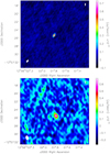 |
Fig. 1. VLA observations of the central binary VHS 1256−1257 AB. The size of the radio beam is shown in the lower left corner of each panel. Upper panel: Stokes I image of the 6 GHz data set. Lower panel: same as upper panel, but for the 33 GHz data set. |
We also used CASA for the reduction of eMerlin data, following the standard procedures. To improve the sensitivity, we combined the three consecutive dates into one data set allowing us to reach a 1σ rms of 20 μJy beam−1. No detection was found at the expected position.
Data calibration for NOEMA data was performed with the GILDAS–CLIC software (sep-2019 version)2. The continuum was obtained by averaging line–free channels over the 7.744 MHz width (USB) centered at 230.0 GHz. No emission was found at the expected position of the central binary VHS 1256−1257AB with a 1σ rms of 51 μJy beam−1.
The calibration of the ALMA data followed the standard ALMA quality assurance procedure for Cycle 6 based on the CASA data analysis package version 5.4.-70 (McMullin et al. 2007). We obtained our final image by combining all spectral channels into one image using the tclean task of the same CASA package in mfs mode. VHS 1256−1257 data were imaged as a single field with a pixel size of 0.16 arcsec and natural weighting in order to optimise the point-source sensitivity. No significant sources were found in the final image, resulting in a rms of 40 μJy beam−1 at the location of VHS 1256−1257AB.
To extract the flux density of VHS 1256−1257AB on each map where the source is detected, we used the CASA task imfit to fit an elliptical Gaussian with the size of the synthesized beam and centered at the peak intensity. We also searched for short-term variability on the detected radio emissions: (i) for two-day observations (VLA 33 GHz data), we obtained images and flux densities for each day separately; (ii) we analyzed the interferometric visibilities using the AIPS task DFTPL, which plots the discrete Fourier transform of the complex visibilities for any arbitrary point as a function of time. When necessary, we converted the CASA visibility data set to a UVFITS file using the task exportuvfits. To find a balance between signal-to-noise ratio and temporal resolution, we ran DFTPL with an interval of 60 s.
4. Results
Radio emission from an unresolved source is detected in both VLA observations. The locations of emission coincide with the expected positions of the binary VHS 1256−1256AB, according to the coordinates, proper motion, and parallax given in Gauza et al. (2015), Guirado et al. (2018), and Dupuy et al. (2020). The Stokes I flux density over the whole bandwidth was 73 ± 4 μJy and 83 ± 3 μJy for 6 GHz and 33 GHz, respectively. Circularly polarized flux density was not detected at such frequencies. As an upper limit to the fraction of circular polarisation, we computed the value of 3 × (rms of Stokes V flux density)/(Stokes I flux density), yielding 0.12 and 0.25 for the 6 GHz and 33 GHz data sets, respectively.
Figure 2 shows the temporal evolution of VHS 1256−1257AB flux density (Stokes I and Stokes V) at 6 GHz. The average values are 78 μJy and 4 μJy with a standard deviations of 37 μJy and 38 μJy for total and circular flux density, respectively. At the beginning of the observation, a few points show abnormally low total flux densities, which are likely indicative of an observational effect rather than any physical phenomenon. Throughout the observing time, the total flux density does not present any hints of bursting emission and no significant circular polarization is seen (as previously anticipated). To check for low-level periodic signals, we computed a generalized Lomb-Scargle periodogram (GLS; see Appendix B) and found the maximum power to be a 2σ peak with a period of 15.7 ± 0.3 min. We do not consider this peak to be significant; therefore, the data are consistent with quiescent emission. Figure 3 shows a similar plot for the VLA observation at 33 GHz. In this case, no significant temporal variability is detected within each observing day or between them (with a maximum peak in the GLS of 1.3σ). This indicates that the radio emission from VHS 1256−1256AB at this frequency remains stable for at least nine days.
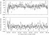 |
Fig. 2. Time evolution of flux density in VHS 1256−1257 at 6 GHz. Upper panel: points show the total flux density (Stokes I) averaged every 60 s, with a mean value of 78 μJy (plotted as a dashed line) and with a standard deviation of 37 μJy (plotted as a gray shadow). Lower panel: same as upper panel, but for Stokes V. The mean and standard deviation values in this case are 4 μJy and 38 μJy, respectively. |
The 6 GHz data clearly match the spectral behavior from Guirado et al. (2018) 10 GHz data (see Fig. 4). There are two particular images, one with bandwidth from 7.97 GHz to 8.62 GHz (10 GHz published data) and the other from 7.75 GHz to 7.90 GHz (6 GHz new data), which are extremely close in frequency. Despite both observations being almost three years apart, the integrated flux densities have remained almost the same: 75 ± 24 μJy (15 May 2015) to 73 ± 13 μJy (13 April 2018), emphasizing the stability of the radio emission not only on scales of days (as seen in Fig. 3), but on scales of years. The turnover frequency, that is, the frequency at which the source transitions from optically thick to optically thin, was estimated to be between 5 and 8.5 GHz (Guirado et al. 2018). Our new data seem to favor the lower frequency range.
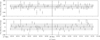 |
Fig. 3. Same as Fig. 2, but for the VLA 33 GHz observations. Mean and standard deviation values are 49 and 58 μJy (Stokes I) and 7 and 89 μJy (Stokes V). |
Motivated by previous estimations of the peak emission from the binary at 5.0–8.5 GHz, we obtained VLBI data at 5 GHz. These observations did not detect any compact radio emission at the expected position with a 1σ upper limit of 10 μJy beam−1. We also found no detection of radio emission at 230 GHz (NOEMA) and 345 GHz (ALMA), placing strong upper limits of 51 and 40 μJy beam−1, respectively. The implications of these non-detections are discussed in the next section.
5. Discussion
5.1. Constraints from the VLBI no-detections
The fact that our results show quiescent emission from the central binary that is stable up to almost three years (see Sect. 4) renders the time variability scenario unlikely to explain such non-detection. This is because VHS 1256−1257AB was observed and detected with the VLA (at a very similar frequency) only ∼6 months before the EVN observation, and only a few weeks apart in the case of VLA 33 GHz observations. Consequently, new scenarios must be considered. The first one that we propose is that of an over-resolved flux component that the EVN and eMerlin are not able to recover due to their higher angular resolution. The second scenario assumes that the detected VLA radio emission comes not from one but from both components of the binary.
Under the assumption that the lack of detection with VLBI is due to an over-resolved component, we can obtain an estimation for the size of the emitting region by taking into account both VLA 6 GHz and the EVN 5 GHz observations. From the VLA data set, we created an image centered at 5 GHz with a bandwidth of 200 MHz to imitate the EVN observation in terms of central frequency and bandwidth. In this case, we detected VHS 1256−1257AB as an unresolved source with a total flux density of 69 ± 7 μJy (rms of 6 μJy beam−1) and with a synthesized beam of 0.79″ × 0.41″. At a distance of 22.2 parsecs, this beam value imposes a maximum size for the emitting region of approximately 13 AU. To estimate a lower bound, we simulated an EVN array with the shortest projected baselines possible so that the resulting image would have an rms of 14 μJy beam−1. With this rms, we should be able to detect the 69 μJy (5σ) total flux density recovered from the VLA image, in the case that it is present. The maximum projected baseline was 2 × 10⁷λ. No detection on this image implies that the size of the emitting region must be larger than 10 mas (0.22 AU or 47 R⊙). If we consider a 3σ limit, the minimum region size would be ∼20 mas (0.44 AU or 95 R⊙). With the separation between components being 0.1″ (Stone et al. 2016), the emitting region size must be between 0.2 and 6 times such a separation. We notice that the higher rms of the eMerlin observations prevents us from repeating similar simulations that would have yielded a more stringent low bound.
Additionally, we must consider the scenario where the detected radio emission in our VLA observations comes from both of the components of the binary rather than just one. In this case, with a 50 μJy beam−1 5σ rms in our EVN observations and a 69 ± 7 μJy total flux density from the VLA equivalent bandwidth image, we estimate the maximum flux ratio between the binary components to be 2.7. The sizes of the emitting regions in this scenario would not need to fit in the values given in the over-resolved scenario. Assuming that both components contribute equally and that they have similar sizes (from 0.12 R⊙ to 0.14 R⊙, according to the age and mass ranges given in Sect. 1; Chabrier et al. 2000), we calculated a brightness temperature of 4.2−5.7 × 10⁹ K for the 6 GHz detection and 1.6−2.1 × 10⁸ K for the 33 GHz detection; both values, in principle, are consistent with synchrotron or gyrosynchrotron nonthermal radio emission (Dulk 1985). However, the spectral analysis of the data in Fig. 4 must be taken into account before assigning an emission mechanism, as we discuss in Sect. 5.3.
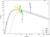 |
Fig. 4. Total flux density of VHS 1256−1257AB from VLA observations updated with our new data and with published data (Guirado et al. 2018) on a smaller bandwidth sampling (circles). Different colors indicate different bands: 1.4 GHz (red), 6 GHz (yellow), 10 GHz (green), 33 GHz (blue), 230 GHz, and 345 GHz (gray). 3σ non-detections are plotted as arrows. Lines represent different gyrosynchrotron models with δ = 1.36 (see Sect. 5.3.1): dotted line for localized emitting region at the stellar surface with size of 1 R* (LES1) and dashed and dash-dot lines for radiation belts with B0 = 2000 G (RB2) and B0 = 3000 G (RB3), respectively. |
Therefore, our VLA detections and VLBI non-detections indicate that either both components of the central binary emit at 5 GHz with a flux ratio ≲2.7 (in which case, no precise estimate of the size of the emitting region can be obtained), or, if the difference is larger, meaning a single component dominates the radio emission, the VLA 6 GHz detection would come from a region with possible sizes raging from ∼20 mas (∼730 R*) up to ∼600 mas (∼21 900 R*). These source sizes seem improbable and, consequently, the detected radio emission is likely to originate from both components with a flux ratio ≲2.7.
5.2. Constraints from short-term stability
Figure 2 demonstrates the lack of short-term variability on this binary over 4 h, indicating that the emitting region is not hidden during such a period of time. Recently, the rotation periods for each component have been obtained through the analysis of TESS data (2.0782 ± 0.0004 h and 2.1342 ± 0.0003 h; Miles-Páez 2021). There is no variability with such periods reproduced in our data (see Sect. 4), which indicates that the same emitting region is seen over almost two rotation periods.
The lack of short-term variability at radio wavelengths could be explained if the binary was observed with a pole-on configuration and if the detected radio emission originated in the polar caps of either or both components. In such scenario, no modulation of the radio emission is expected. However, Zhou et al. (2020) found that for VHS 1256−1257b sin i ≈ 1; that is, the L7 companion is viewed equatorially. A similar result was recently found for each component of the central binary (Miles-Páez 2021). Consequently, Fig. 2 should show a rotational modulation as seen in other UCDs. LP 349−25 represents an exception to this norm, showing a similar short-term stability during the entire rotation period (Osten et al. 2009). Alternative scenarios to explain the lack of rotational modulation in LP 349−25 are the following: (i) magnetic structures located at the surface of one or both components with a high degree of homogeneity; (ii) emission coming from both components emitting out of phase so that the detected radio emission remains constant (in the case of VHS 1256−1257AB, as in LP 349−25, this unlikely scenario would imply that the two components are tidally locked or that information can be communicated on timescales of < 60 s); (iii) a circumbinary radio-emitting structure, which also seems improbable for VHS 1256−1257AB given the great separation between components (∼3600 R*; Stone et al. 2016). We therefore discarded this scenario.
An alternative, better-suited scenario capable of explaining the lack of rotational modulation is that where the radio emission is originating at radiation belts around at least one of the components in a similar fashion to the magnetospheres of magnetic chemically peculiar (MCP) stars. These main-sequence stars (spectral type A/B) possess a mainly dipolar magnetic field with strengths of ∼kG. About 1 in 4 MCP stars emit at radio wavelengths (Leone et al. 1994), and the origin of such radio emission is usually linked to gyrosynchrotron emission from nonthermal electrons moving in a magnetospheric cavity with tens of stellar radii in size (see Fig. 1 of Trigilio et al. 2004). In some of these stars, the radio emission is modulated by the stellar rotation as the orientation of the magnetosphere changes with respect to the line of sight as a function of the rotational phase (oblique rotator model; Trigilio et al. 2004). This model has also been applied to the light curve of the UCD 2MASS J13142039+1320011 (McLean et al. 2011) and to TVLM 513−46546 (Leto et al. 2017). In the case of VHS 1256−1257AB, the total lack of rotational modulation could be explained if the object and belts were seen equatorially (i.e., rotation and magnetic axes perpendicular to our line of sight), which is in agreement with the measurements of Zhou et al. (2020) and Miles-Páez (2021), and would imply no modulation during the entire rotation of the object. The size of the radiation belts would not need to be as large as those present in MCP stars, as sizes similar to Jupiter’s radiation belts (de Pater 1981) or slightly larger have been used to describe the field topology of UCD magnetospheres (Metodieva et al. 2017).
Independently of the spatial origin of the radio emission, if we assume the typical conditions seen in other UCDs, that is, radio emission produced by individual bursts originating in a localized region then, in a similar fashion to LP 349−25 (Osten et al. 2009), we can constrain the electron density ne in the case where the energy loss is due to collisions in a high-density environment (Eq. (2.6.20) of Benz 2002). For a temperature > 106 K and a 10 keV particle to have a collisional deflection time of > 4 h (< 60 s), ne ≲ 6 × 10⁵ (≳2 × 10⁷) cm−3 is necessary. If the energy loss is due to radiation losses in a high magnetic field region, the timescales for radiation loss (tr; Petrosian 1985) imply magnetic field strengths B ≲ 210 G (tr > 4 h) and B ≳ 4 kG (tr < 60 s) for a 10 keV electron. As such, if the origin of the detected radio emission is akin to other UCDs, we constrained the plasma conditions to be either ne ≲ 6 × 105 cm−3 or ne ≳ 2 × 107 cm−3 and B ≲ 210 G or B ≳ 4 kG.
Therefore, the lack of short-term variability points to either the presence of radiation belts around at least one of the components of VHS 1256−1257AB that would be seen equatorially, or to a region on the stellar surface with a high degree of homogeneity. In any of the cases, if the emission region is localized, the plasma conditions would be constrained by the values given at the end of the previous paragraph.
5.3. Constraints from spectral analysis
Quiescent emission of UCDs is successfully interpreted as incoherent gyrosynchrotron emission of energetic electrons in a mild magnetic field (e.g., Berger et al. 2001; Osten et al. 2009). At low frequencies (optically thick), the gyrosynchrotron emission spectrum shows a positive slope, while at higher frequencies (optically thin) a negative slope is seen. As previously stated, the VLA detection at 6 GHz (C-band) is compatible with the spectrum presented by Guirado et al. (2018), despite the data having been collected almost three years apart (see Fig. 4). This, together with non-detection at 1.4 GHz (L-band), led us to formulate the self-absorption hypothesis in which gyrosynchrotron radiation from a power-law energy distribution of electrons would explain the observed spectrum between 1 and 12 GHz, with a turnover frequency located around 5 GHz. This mechanism produces a relatively low degree of circular polarisation (Dulk 1985), which is also seen in our observations. Our 33 GHz (Ka-band) detection, however, presents a challenge to this hypothesis as no detectable emission is expected at such frequencies, but a clear component still appears in our map (Fig. 1). To explain the broadband spectrum of VHS 1256−1257AB, we considered a few scenarios that we discuss in the following sections.
5.3.1. Single-spectrum hypothesis: Flat spectral index
The first scenario consists of an almost flat spectral index, α, for the optically thin regime that would encompass the 33 GHz detection. This is certainly far from the α = −1.1 reported by (Guirado et al. 2018) from simultaneous observations between 8 and 12 GHz, but it is in an overall better agreement with observations ranging from 4 GHz to 37 GHz, while also explaining the non-detections at NOEMA and ALMA frequencies. We now discuss the different mechanisms able to produce an almost flat spectral index.
In the case of thermal bremsstrahlung being T the temperature of the thermal plasma, A the source area, L the characteristic length scale along the line of sight, ne the electron density, and VEM the volume emission measure ( ), the flux density expected for a source located at 22.2 pc due to optically thin thermal bremsstrahlung can be expressed as:
 (1)
(1)
where the VEM has units of cm−3 and T is in units of K. If the detected radio emission comes from a chromosphere or corona at temperatures 104 − 106 K, then the volume emission measure would range from 5 × 1052 to 5 × 1053 cm−3. This range is much larger than the X-ray VEM observed in, for example, UV Ceti (2.6 × 1050 cm−3; Kundu et al. 1987) and other dMe stars (e.g., Schmitt et al. 1990; White et al. 1994). In those cases where VEM and T are known, optically thin bremsstrahlung radio fluxes from the coronas of UCDs are estimated to be orders of magnitude below the observed fluxes (Gary & Linsky 1981; Leto et al. 2000). Unless VHS 1256−1257 AB represents a special case, we must conclude that optically thin free-free emission from the corona is probably too weak to produce the measured radio fluxes. We can also dismiss optically thick thermal emission from active regions in the stellar surface or corona akin to ϵ Eridani (Bastian et al. 2018) as the observed brightness temperature in our case is TB ≫ 106 K (see Sect. 5.1).
Another possible source of free-free emission is the stellar wind. As an approximation, we assumed an isothermal, spherically symmetric, fully ionized wind originating in one of the components exhibiting spectral behavior Sν ∝ ν0.6 for the optically thick part and Sν ∝ ν−0.1 once the spectrum becomes optically thin (Panagia & Felli 1975). Using Eqs. (9) and (10) from Rodríguez et al. (2019), we estimate that a free–free emission from a stellar wind with turnover frequency located at 4 GHz and able to reproduce our 33 GHz detection would imply an electron temperature Te ∼ 3 × 10⁵ K, and a wind mass-loss rate of Ṁw ∼ 2 × 10⁻¹⁰ M⊙ yr−1, under the assumption that the wind velocity is approximately equal to the velocity escape ∼520 km s−1. The estimated mass-loss rate is ∼1000 greater than the predictions from models of winds from cool stars driven by Alfvén waves and turbulence (Cranmer & Saar 2011), and even greater than the mass-loss rate that would explain the observed spectrum in the much bigger star ϵ Eridani (Rodríguez et al. 2019; Suresh et al. 2020). For this reason, we conclude that the flat spectrum in VHS 1256−1257AB cannot be succesfully reproduced by free–free stellar wind emission.
The flatness of the spectrum could also be reproduced if the detected emission originates in a number of small active regions where self-absorbed nonthermal gyrosynchrotron emission is produced with a different turnover frequency for each region (White et al. 1989). Then, it is possible to obtain an approximately flat spectrum with bumps on it. This, however, seems highly unlikely, as turnover frequencies as large as 33 GHz would imply magnetic field strengths of ∼15 kG using the relation B(kG)≈0.151ν(GHz)1.316 (White et al. 1989).
Nonthermal gyrosynchrotron emission from a power-law energy distribution of electrons can also reproduce the required flatness of the spectrum. Fixing the optically thin spectral index to α = 0, one can obtain the spectral index of energetic electrons, δ, using the following formula (Dulk 1985):
 (2)
(2)
where ϑ is the angle between the magnetic field and the observer direction, vB is the electron gyrofrequency, B is the magnetic field, ne is the concentration of energetic electrons in the source, d is the thickness of the source projected on the observer, s is the visible area of the source, and R is the distance to the radio emission source. This would imply a particularly hard spectrum of nonthermal electrons with δ ≈ 1.36 (where dN/dE ∝ E−δ). Using this value, we performed numerical simulations of the expected gyrosynchrotron emission in the magnetosphere of VHS 1256−1257AB (see Appendix A) in two different spatial configurations: a region at the stellar surface, and radiation belts akin to Jupiter’s. The first one assumes a localized emitting region at the stellar surface which, to concur with the lack of short term variability, must always be present during our observations; for example, a polar cap seen equatorially. As a rough estimation, we fixed the size of the emitting region to be the radius of one component (0.12 R⊙, see Sect. 1). The best fit was found with B = 140 ± 50 G and ne = 2.154 ± 0.003 × 104 cm−3, where the error bars indicate the value differences between each simulation. The second configuration assumes gyrosynchrotron radio emission originating at radiation belts (see discussion in Sect. 5.2 and details in Appendix A). In this case, the best values are B = 140 ± 50 G, ne = 680 ± 30 cm−3, and B = 140 ± 50 G and ne = 320 ± 30 cm−3 for a maximum magnetic field strength at the surface level (B0) of G and 3000 G, respectively. These models are shown in Fig. 4 and indicate that a spatial configuration of radiation belts (with approximately the same size as the stellar radius) produces an overall better fit than a localized region.
Independently from its spatial origin, the values for B and ne obtained with the simulations are in agreement with the estimations that can be made using solely the detections at the extremes of the frequency range; i.e., 5 GHz and 33 GHz. Typically, gyrosynchrotron emission arises at frequencies of ν = sνB, where the harmonic number, s, takes values from 10−100 and νB is the electron gyrofrequency given by νB = 2.8 × 10⁶B, with B expressed in Gauss and νB in Hz. For the 5 GHz and 33 GHz detections, gyrosynchrotron emission implies magnetic field strengths in the radio-emitting source of 18−180 G and 120−1200 G, respectively. In the presence of plasma, gyrosynchrotron emission at harmonic s becomes suppressed at νp ≳ νBs−1/2 (Dulk 1985). Assuming that the 5 GHz detection is caused by this mechanism with harmonics ranging from 10 to 100, this implies ne ≲ 3.1 × 108 cm−3 and ne ≲ 3.1 × 105 cm−3, respectively. Therefore, if the detected 5 GHz radio emission is produced by the gyrosynchrotron mechanism involving high-value harmonics (s ∼ 100), our detection allows us to dismiss the ne ≳ 2 × 107 cm−3 estimation given in Sect. 5.2 and place an upper limit for the electron density of ne ≲ 3.1 × 105 cm−3. As such, both constraints for B and ne are met in our simulations. For B ≈ 140 G, the detection at 33 GHz indicates that the bulk of the gyrosynchrotron emission originates at s ∼ 80, which implies ne ≲ 2.6 × 107 cm−3.
Previously we argued that despite incorporating data taken almost three years apart from our new observations (green points in Fig. 4), the part of the spectrum between 4 and 12 GHz could be treated as if the data were simultaneous. We ran the simulations for the gyrosynchrotron scenarios described above, but utilizing solely data taken a few months apart; that is, the 6 GHz and 33 GHz data sets. The best simulations for each scenario did not differ from those using 6 GHz, 10 GHz, and 33 GHz observations. As such, a plausible scenario to explain the broad-band spectrum of VHS 1256−1257AB is gyrosynchrotron emission coming from radiation belts around (at least) one of the components.
Additional scenarios are best explained considering the spectrum as a superposition of a low frequency part (LF) below 15 GHz and a high frequency part (HF) above 15 GHz. We now discuss them separately.
5.3.2. Composite-spectrum hypothesis: The LF regime
There are two possible mechamisms to explain the LF regime of the spectrum: nonthermal gyrosynchrotron and optically thick thermal gyroresonance. As previously stated, quiescent emission is usually interpreted as nonthermal gyrosynchrotron emission from a power-law energy distribution of electrons. Limiting the frequencies to the LF part of the spectrum, we repeated the numerical simulations described in Sect. 5.3.1 for the same scenarios, that is, a one-stellar radius region at the surface of one component and radiation belts around at least one component of the binary. However, this time we did not fix the spectral index of energetic electrons, δ. In the case of a localized emitting region, we found no fit better than that presented in Sect. 5.3.1. In the case of radiation belts, the best fit corresponds to B = 140 ± 50 G, ne = 1.000 ± 0.003 × 104 cm−3, δ = 2.1 ± 0.2 for B0 = 2000 G, B = 140 ± 50 G, ne = 1.779 ± 0.003 × 104 cm−3, and δ = 1.8 ± 0.2 for B0 = 3000 G. These models are shown in Fig. 5 and indicate that the LF part of the spectrum of VHS 1256−1257AB can be explained with nonthermal gyrosynchrotron emission originating in radiation belts around at least one of the components.
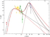 |
Fig. 5. Same as Fig. 4, but this time lines represent the different gyrosynchrotron models discussed in Sects. 5.3.2 and 5.3.3. Red and black dashed lines for radiation belts at LF with B0 = 2000 G and B0 = 3000 G, respectively; red and black dotted line for a localized emission at HF and radiation belts with B0 = 3000 G, respectively; red solid line for the combination of radiation belts with B0 = 2000 G at LF and B0 = 3000 G at HF; black solid line for the combination of radiation belts with B0 = 2000 G at LF and a localized region at HF. |
As stated in Sect. 5.3.1, the 5 GHz detection implies values of the magnetic field strength in the radio-emitting source B = 18−180 G for gyrosynchrotron emission with harmonics of s = 10−100, respectively. At a frequency of 12 GHz, this translates to B = 43−430 G. Therefore, the best-fit values for B in any of the scenarios discussed in the simulations are in agreement with these ranges.
An alternative scenario that could explain the LF part of the spectrum is optically thick, thermal gyroresonance radiation, that is, nonrelativistic electrons spiralling around magnetic field lines. The absorption coefficient for this mechanism is (Melrose et al. 1985)
 (3)
(3)
where νp = (ne2/(πme))1/2 is the plasma frequency, s the harmonic number, θ the angle between the magnetic field and the line of sight, β0 = (2kT/(mec2))1/2, and νB = eB/(2πmec) is the gyrofrequency. For an optically thick emission, and assuming a critical optical depth of τ = κl > 2, where l = 2ΛBβ0 cos θ is the resonance length and ΛB the magnetic scale height, Gudel & Benz (1989) found that the emission observed in UV Ceti could be reproduced by harmonics s = 4−6. Leto et al. (2000) found that the dMe stars V1054 Oph and AU Mic present a similar harmonic range up to where the plasma component is optically thick for gyroresonance emission. Following these results, and due to the lack of VEM and T measurements, we took s = 4 as a mere illustrative case.
The observed α ≈ −1.1 in the LF part could result from a contraction of the source size with frequency: Sν ∼ r2ν2 ∼ ν−1.1 from where r ∼ ν−1.55. Since the frequency of cyclotron emission is proportional to the magnetic field, we find that B ∼ ν ∼ r−0.65. To explain the detections at 4 GHz and 12 GHz, the gyrofrequency equation implies magnetic field strengths between 360 G and 1070 G (s = 4). With B = B0 r−0.65, a photospheric value of B0 = 1070 G implies a source radius of 5.4 R* for B = 360 G. This value does not agree with the constraints obtained from Sect. 5.1 for emission coming mainly from one of the components of the binary, reinforcing the results that the observed emission is likely coming from both components in the case of optically thick, thermal gyroresonance radiation. According to Eq. (5) of Leto et al. (2000), a source with radius of 5.4 R* would need to have T ≈ 8.0 × 10⁷ K to produce the measured emission at 5 GHz (half for equal contribution of both components). This value is an order of magnitude higher than the plasma temperatures from X-ray data analysis found in the literature for the cool plasma component of dMe stars (e.g., Schmitt et al. 1990; Giampapa et al. 1996; Sciortino et al. 1999) and UCDs (e.g., Robrade & Schmitt 2009; Stelzer et al. 2012) but similar to the hot plasma component. This optically thick gyroresonance scenario, however, runs into a problem. Gary & Linsky (1981) proposed a scaling law for the magnetic field in the outer atmospheres of late type stars where B ∼ r−2, which was found to be valid for UV Cet, V 1054 Oph, and EV Lac, but not for AU Mic, where magnetic field strength decreased with radial distance much more rapidly (Leto et al. 2000). Even the slower radial dependence of the magnetic field above active regions in our Sun falls as B ∼ r−1.5 (Dulk & McLean 1978). Therefore, although the current observations cannot rule out optically thick gyroresonance, we warn the reader that, in such cases, the presence of a magnetic field with a very low radial dependence needs to be explained.
5.3.3. Composite-spectrum hypothesis: The HF regime
Due to the young age of this binary, we considered the possible contribution that a debris disk surrounding VHS 1256−1257AB would have to the HF part. In principle, one can find parameters of such a disk that would reproduce the density flux recovered in our 33 GHz image. However, this hypothesis was quickly dismissed with the ALMA data. We used the BT-Settl photospheric model (Baraffe et al. 2015) valid for a cool dwarf with solar metallicity, Teff = 2600 K, and log g = 5.0 [cm s−2], which are the parameters expected for an M7.5 source with an age of a few hundred million years (Chabrier et al. 2000). This photospheric flux density was then combined with the emission of a putative thin dusty disk with the parameters of the famous AU Mic debris disk (Liu 2004); that is, 0.89 Mlunar, a grain size of 100 μm, and a temperature of 40 K. We found that the expected flux density at 340 GHz would be ten times larger than our 3σ constraint from the ALMA data. Therefore, our observations dismissed the presence of a massive disc similar to that of AU Mic and, consequently, led us to consider alternative scenarios.
Up to this point, we assumed that the detected radio emission, if it is nonthermal gyrosynchrotron, is coming from only one of the components of the binary or from both components but with equal B, nb, and δ. We may also consider the scenario where each component contributes differently not only in terms of integrated flux but in terms of the physical conditions. In this manner, we hypothesize that one component may be the responsible for the radio emission in the LF regime, while the other one may be responsible for it in the HF regime. To test this hypothesis, we ran the gyrosynchrotron simulations described above for the cases of a localized radio emission and a radiation belt with B0 = 3000 G. The best fit for a localized emission corresponds to B = 1760 ± 50 G, ne = 2.0000 ± 0.0003 × 105 cm−3, and δ = 2.8 ± 0.2. For a radiation belt with B0 = 3000 G, we found B = 1050 ± 50 G, ne = 4.70000 ± 0.00003 × 106 cm−3, and δ = 3.0 ± 0.2 (see Fig. 5). The localized region value for the magnetic field strength does not meet the constraint of Sect. 5.2, if the emision is similar to other UCDs. As such, if the emission at 33 GHz is due to nonthermal gyrosynchrotron coming from one of the components, our data favor a radiation belt as the spatial origin.
Can the HF part be explained by thermal gyrosynchrotron? This mechanism is usually expected in highly magnetized stars (B∼ kG) that posses very hot plasma (T ∼ 108 K). Assuming a homogeneous source, this mechanism would produce an optically thick spectral index ∝ν2, which would peak at frequencies of ≥10 GHz and a steep optically thin spectral index ∝ν−8 (Güdel 2002). With this spectral behavior, thermal gyrosynchrotron could be responsible for the emission seen at 33 GHz, and given its ultra-steep behavior, it would be almost imperceptible at NOEMA and ALMA frequencies. However, the fact plasma temperatures as high as 108 K are needed and that a very high circular polarisation (≥30%) is expected from this mechanism (Matthews 2019) while no detectable polarisation is seen in VHS 1256−1257AB renders thermal gyrosynchrotron very unlikely. Perhaps this is thermal gyroresonance emission akin to that invoked to explain the U-shaped spectra of AU Mic (Cox 1985), UV Ceti (Gudel & Benz 1989), ER Vul (García-Sánchez et al. 2003), and other dMe stars (Gudel et al. 1996; Leto et al. 2000). In these objects, the emission is assumed to come from the X-ray-emitting plasma (which is optically thick) and is responsible for the increase in flux seen after 5−8 GHz. However, our observations show a decrease in flux not only at 4−5 GHz but also at > 33 GHz, indicating that the emission at these higher frequencies should come from an optically thin plasma. Is this a reasonable scenario? For a range of objects where both T and VEM are known, White et al. (1994) estimated that thermal gyroresonance is optically thick unless the magnetic scale height is as follows: ΛB ≪ 0.01 R*. In such a case, a clear eclipse signature of the hot X-ray plasma would be expected, while none is seen during our observations. Consequently, we conclude that optically thin gyroresonance emission is not a plausible mechanism for the HF part of the spectrum of VHS 1256−1257.
One final alternative mechanism to consider is the electron cyclotron maser instability (ECMI) mechanism (as proposed by Hallinan et al. 2008, to explain the broadband, non-flaring radio emission of UCDs). This emission would have strong cut-offs at low and high frequencies, justifying the non-detection at 1.4 GHz as well as those at NOEMA and ALMA frequencies. However, our detection at 33 GHz makes this scenario highly unlikely, since it would imply the existence of magnetic field strengths of ≥11 kG, which is an order of magnitude higher than that reported in Guirado et al. (2018) and also much larger than theoretical limits on the surface field strengths of low-mass stars (Feiden & Chaboyer 2014). Additionally, this mechanism is expected to produce radio emission with a high degree of circular polarisation, which is not the case for our observations.
Therefore, a distribution of electrons (ne ≈ 106.5 cm−3) following a power-law (δ ≈ 3.0) in the presence of a strong magnetic field (B ≈ 1 kG) and located at a radiation belt around one of the components of VHS 1256−1257AB would produce nonthermal gyrosynchrotron emission in the HF regime similar to that detected in our observations.
5.4. Combining all the constraints
From the discussions of Sects. 5.2 and 5.3, we conclude that one of the most plausible scenarios that reproduces the broad-brand spectrum of this object is gyrosynchrotron emission from a power-law distribution of electrons where both components of the binary possess different physical conditions (B, ne and δ). When limiting the emission to originate in only one of the components or, equivalently, in both components but with the same B, ne and δ, we found an acceptable fit with emission originating from radiation belts (Fig. 4). This hypothesis fits well with the spatial constraint from Sect. 5.1. On the other hand, a composite-spectrum hypothesis produces a considerably better fit (Fig. 5), particularly when we allow each component of the binary to have a different set of free parameters: B, ne, and δ. This is not unexpected as we are effectively doubling the number of degrees of freedom. In this scenario, the emission of one of the components would originate in radiation belts peaking at ∼4 GHz, while emission from the other component would peak at ∼30 GHz and would also originate in radiation belts around it. Although this scenario is in agreement with the lack of short-term variability (Sect. 5.2), it is at odds with the spatial constraints obtained from the lack of detection with VLBI (Sect. 5.1). In this configuration, the flux ratio between the binary components at 5 GHz would be much larger than 2.7, and, therefore, the VLA 6 GHz detection would need to come from a region of 730 R* < R < 21 900 R* in size; assuming there is no temporal variability, this size is much larger than the radiation belts’ diameters, which definitely does not favor this scenario.
Another possible scenario capable of concurring with all the constraints discussed above is the combination of optically thick gyroresonance at LF and nonthermal gyrosynchrotron emission at HF. In this case, an explanation for the slow radial dependence of the magnetic field (B ∼ r−0.65) needs to be given for the LF regime. At the HF regime, no strict constraints apply, as a localized emitting region or radiation belts around one or two of the components could be plausible.
Therefore, if the measured stability in radio emission over almost three years is real, current VLA and VLBI observations of VHS 1256−1257AB could be explained by nonthermal gyrosynchrotron radio emission coming from both components and originating in equatorial radiation belts around each UCD. Although a combination of optically thick gyroresonance and nonthermal gyrosynchrotron emission could also be a possible explanation, our analysis renders such a scenario less likely.
6. Conclusions
We present new detections of radio emission in the central binary of the substellar triple system VHS 1256−1257 centered at 6 GHz and 33 GHz. This emission is not detected with VLBI arrays. We also placed strong upper limits to the radio emission of this binary at 230 GHz and 345 GHz. Both detections at 6 GHz and 33 GHz present a Stokes I flux density of 73 ± 4 μJy and 83 ± 13 μJy, respectively, with no detectable circular polarisation or pulses. We now summarize the constraints that arise from the observations.
-
The emission at 33 GHz appears stable over a period of nine days, whereas that at 6 GHz is compatible with stability for almost three years.
-
The lack of detection with VLBI arrays implies that the radio emission produced at 4–8 GHz originates either in both components of the central binary with a flux ratio of ≲2.7 or in a region with between ∼20 mas and ∼600 mas in size (∼730 and ∼21 900 R*).
-
The lack of detection with ALMA dismisses the presence of a significant or massive debris disk similar to that of AU Mic.
-
Both 6 GHz and 33 GHz observations lack any density flux variability during the observations, which has some implications as well. Either the detected flux is emitted in radiation belts around each component of the binary or in a region with a high degree of homogeneity located on the stellar surface.
-
If the emission comes from radiation belts, the rotation and magnetic axes should be perpendicular to our line of sight; that is, they would be seen equatorially.
-
If the emission comes from a localized radio emission (as seen in other UCDs), the plasma conditions must be ne ≲ 6 × 105 cm−3 or ne ≳ 2 × 107 cm−3 and B ≲ 210 G or B ≳ 4 kG.
We discuss various scenarios to explain the spectral behavior of VHS 1256−1257AB. Taking into account the constraints described above, we have narrowed them down to two: (i) a combination of optically thick gyroresonance and nonthermal gyrosynchrotron. This scenario seems unlikely as the radial dependence of the magnetic field is uncommonly slow (B ∼ r−0.65) and would need a well-reasoned justification; (ii) a nonthermal gyrosynchrotron mechanism operating at radiation belts around both components of the binary, which would be seen equatorially. Plausible conditions for this more likely scenario are a low plasma density (ne = 300−700 cm−3), a moderate magnetic field strength (B ≈ 140 G, assuming a ∼kG maximum strength on the stellar surface), and a power-law distribution of electrons with δ fixed at 1.36. These values should not be taken as definitive, as the simulations have only been used as a proof of feasibility. New multifrequency observations (at 10−30 GHz) of this intriguing system would allow for a more certain determination of both the emission mechanisms involved and the physical parameters, shedding some light on the question of how UCD emit at radio frequencies.
https://github.com/mzechmeister/GLS
Acknowledgments
We sincerely thank the anonymous referee for his/her very useful and constructive criticisms and suggestions. This paper is based on observations carried out with the IRAM NOEMA interferometer and the IRAM 30-m telescope. IRAM is supported by INSU/CNRS (France), MPG (Germany), and IGN (Spain). JBC and JCG were partially supported by the Spanish MINECO projects AYA2015-63939-C2-2-P, PGC2018-098915-B-C22 and by the Generalitat Valenciana project GVPROMETEO2020−080. MPT acknowledges financial support from the State Agency for Research of the Spanish MCIU through the “Center of Excellence Severo Ochoa” award to the Instituto de Astrofísica de Andalucía (SEV-2017-0709) and through grants PGC2018-098915-B-C21 and PID2020-117404GB-C21 (MCI/AEI/FEDER, UE). RA was supported by the Generalitat Valenciana postdoctoral grant APOSTD/2018/177. BG acknowledges support from the UK Science and Technology Facilities Council (STFC) via the Consolidated Grant ST/R000905/1. MRZO and VJSB acknowledge the financial support from PID2019-109522GB-C51 and PID2019-109522GB-C53, respectively.
References
- Baraffe, I., Homeier, D., Allard, F., & Chabrier, G. 2015, A&A, 577, A42 [NASA ADS] [CrossRef] [EDP Sciences] [Google Scholar]
- Bastian, T. S., Villadsen, J., Maps, A., Hallinan, G., & Beasley, A. J. 2018, ApJ, 857, 133 [NASA ADS] [CrossRef] [Google Scholar]
- Benz, A. 2002, Plasma Astrophysics, 2nd edn., 279 [Google Scholar]
- Berger, E. 2002, ApJ, 572, 503 [NASA ADS] [CrossRef] [Google Scholar]
- Berger, E. 2006, ApJ, 648, 629 [NASA ADS] [CrossRef] [Google Scholar]
- Berger, E., Ball, S., Becker, K. M., et al. 2001, Nature, 410, 338 [NASA ADS] [CrossRef] [Google Scholar]
- Berger, E., Rutledge, R. E., Phan-Bao, N., et al. 2009, ApJ, 695, 310 [NASA ADS] [CrossRef] [Google Scholar]
- Biller, B. A., Vos, J., Buenzli, E., et al. 2018, AJ, 155, 95 [NASA ADS] [CrossRef] [Google Scholar]
- Bouy, H., Martín, E. L., Brandner, W., & Bouvier, J. 2005, AJ, 129, 511 [NASA ADS] [CrossRef] [Google Scholar]
- Browning, M. K. 2008, ApJ, 676, 1262 [Google Scholar]
- Chabrier, G., Baraffe, I., Allard, F., & Hauschildt, P. 2000, ApJ, 542, 464 [Google Scholar]
- Christensen, U. R., Holzwarth, V., & Reiners, A. 2009, Nature, 457, 167 [Google Scholar]
- Cox, J. J., & Gibson, D. M. 1985, Thermal Emission and Possible Rotational Modulation in AU Mic, eds. R. M. Hjellming, & D. M. Gibson, 116, 233 [NASA ADS] [Google Scholar]
- Cranmer, S. R., & Saar, S. H. 2011, ApJ, 741, 54 [Google Scholar]
- de Pater, I. 1981, J. Geophys. Res., 86, 3423 [NASA ADS] [CrossRef] [Google Scholar]
- Donati, J.-F., Forveille, T., Collier Cameron, A., et al. 2006, Science, 311, 633 [Google Scholar]
- Dulk, G. A. 1985, ARA&A, 23, 169 [Google Scholar]
- Dulk, G. A., & McLean, D. J. 1978, Sol. Phys., 57, 279 [CrossRef] [Google Scholar]
- Dupuy, T. J., Liu, M. C., Magnier, E. A., et al. 2020, Res. Notes Am. Astron. Soc., 4, 54 [Google Scholar]
- Feiden, G. A., & Chaboyer, B. 2014, ApJ, 789, 53 [NASA ADS] [CrossRef] [Google Scholar]
- Fleishman, G. D., & Kuznetsov, A. A. 2010, ApJ, 721, 1127 [NASA ADS] [CrossRef] [Google Scholar]
- Gaia Collaboration (Brown, A. G. A., et al.) 2021, A&A, 649, A1 [NASA ADS] [CrossRef] [EDP Sciences] [Google Scholar]
- García-Sánchez, J., Paredes, J. M., & Ribó, M. 2003, A&A, 403, 613 [NASA ADS] [CrossRef] [EDP Sciences] [Google Scholar]
- Gary, D. E., & Linsky, J. L. 1981, ApJ, 250, 284 [NASA ADS] [CrossRef] [Google Scholar]
- Gastine, T., Morin, J., Duarte, L., et al. 2013, A&A, 549, L5 [NASA ADS] [CrossRef] [EDP Sciences] [Google Scholar]
- Gauza, B., Béjar, V. J. S., Pérez-Garrido, A., et al. 2015, ApJ, 804, 96 [NASA ADS] [CrossRef] [Google Scholar]
- Giampapa, M. S., Rosner, R., Kashyap, V., et al. 1996, ApJ, 463, 707 [NASA ADS] [CrossRef] [Google Scholar]
- Girard, J. N., Zarka, P., Tasse, C., et al. 2016, A&A, 587, A3 [NASA ADS] [CrossRef] [EDP Sciences] [Google Scholar]
- Gizis, J. E., Faherty, J. K., Liu, M. C., et al. 2012, AJ, 144, 94 [NASA ADS] [CrossRef] [Google Scholar]
- Güdel, M. 2002, ARA&A, 40, 217 [Google Scholar]
- Gudel, M., & Benz, A. O. 1989, A&A, 211, L5 [NASA ADS] [Google Scholar]
- Gudel, M., & Benz, A. O. 1996, in Radio Emission from the Stars and the Sun, eds. A. R. Taylor, & J. M. Paredes, ASP Conf. Ser., 93, 303 [NASA ADS] [Google Scholar]
- Guirado, J. C., Azulay, R., Gauza, B., et al. 2018, A&A, 610, A23 [NASA ADS] [CrossRef] [EDP Sciences] [Google Scholar]
- Hallinan, G., Bourke, S., Lane, C., et al. 2007, ApJ, 663, L25 [NASA ADS] [CrossRef] [Google Scholar]
- Hallinan, G., Antonova, A., Doyle, J. G., et al. 2008, ApJ, 684, 644 [Google Scholar]
- Kao, M. M., Hallinan, G., Pineda, J. S., et al. 2016, ApJ, 818, 24 [NASA ADS] [CrossRef] [Google Scholar]
- Kirkpatrick, J. D., Henry, T. J., & Irwin, M. J. 1997, AJ, 113, 1421 [NASA ADS] [CrossRef] [Google Scholar]
- Kundu, M. R., Jackson, P. D., White, S. M., & Melozzi, M. 1987, ApJ, 312, 822 [NASA ADS] [CrossRef] [Google Scholar]
- Leone, F., Trigilio, C., & Umana, G. 1994, A&A, 283, 908 [NASA ADS] [Google Scholar]
- Leto, G., Pagano, I., Linsky, J. L., Rodonò, M., & Umana, G. 2000, A&A, 359, 1035 [NASA ADS] [Google Scholar]
- Leto, P., Trigilio, C., Buemi, C. S., et al. 2017, MNRAS, 469, 1949 [NASA ADS] [CrossRef] [Google Scholar]
- Lew, B. W. P., Apai, D., Zhou, Y., et al. 2016, ApJ, 829, L32 [NASA ADS] [CrossRef] [Google Scholar]
- Liu, M. C. 2004, Science, 305, 1442 [NASA ADS] [CrossRef] [Google Scholar]
- Liu, M. C., Magnier, E. A., Deacon, N. R., et al. 2013, ApJ, 777, L20 [NASA ADS] [CrossRef] [Google Scholar]
- Marois, C., Macintosh, B., Barman, T., et al. 2008, Science, 322, 1348 [Google Scholar]
- Marois, C., Zuckerman, B., Konopacky, Q. M., Macintosh, B., & Barman, T. 2010, Nature, 468, 1080 [NASA ADS] [CrossRef] [Google Scholar]
- Matthews, L. D. 2019, PASP, 131, 016001 [NASA ADS] [CrossRef] [Google Scholar]
- McLean, M., Berger, E., Irwin, J., Forbrich, J., & Reiners, A. 2011, ApJ, 741, 27 [NASA ADS] [CrossRef] [Google Scholar]
- McMullin, J. P., Waters, B., Schiebel, D., Young, W., & Golap, K. 2007, in Astronomical Data Analysis Software and Systems XVI, eds. R. A. Shaw, F. Hill, & D. J. Bell, ASP Conf. Ser., 376, 127 [Google Scholar]
- Melrose, D. B. 1985, Plasma Emission Mechanisms, eds. D. J. McLean, & N. R. Labrum, 177 [Google Scholar]
- Metodieva, Y. T., Kuznetsov, A. A., Antonova, A. E., et al. 2017, MNRAS, 465, 1995 [NASA ADS] [CrossRef] [Google Scholar]
- Miles-Páez, P. A. 2021, A&A, 651, L7 [NASA ADS] [CrossRef] [EDP Sciences] [Google Scholar]
- Mohanty, S., Basri, G., Shu, F., Allard, F., & Chabrier, G. 2002, ApJ, 571, 469 [NASA ADS] [CrossRef] [Google Scholar]
- Morin, J., Dormy, E., Schrinner, M., & Donati, J. F. 2011, MNRAS, 418, L133 [NASA ADS] [CrossRef] [Google Scholar]
- Osten, R. A., Phan-Bao, N., Hawley, S. L., Reid, I. N., & Ojha, R. 2009, ApJ, 700, 1750 [NASA ADS] [CrossRef] [Google Scholar]
- Panagia, N., & Felli, M. 1975, A&A, 39, 1 [Google Scholar]
- Petrosian, V. 1985, ApJ, 299, 987 [NASA ADS] [CrossRef] [Google Scholar]
- Radigan, J., Jayawardhana, R., Lafrenière, D., et al. 2013, ApJ, 778, 36 [NASA ADS] [CrossRef] [Google Scholar]
- Reiners, A., & Basri, G. 2010, ApJ, 710, 924 [Google Scholar]
- Rich, E. A., Currie, T., Wisniewski, J. P., et al. 2016, ApJ, 830, 114 [NASA ADS] [Google Scholar]
- Robrade, J., & Schmitt, J. H. M. M. 2009, A&A, 496, 229 [NASA ADS] [CrossRef] [EDP Sciences] [Google Scholar]
- Rodríguez, L. F., Lizano, S., Loinard, L., et al. 2019, ApJ, 871, 172 [CrossRef] [Google Scholar]
- Route, M., & Wolszczan, A. 2016, ApJ, 821, L21 [NASA ADS] [CrossRef] [Google Scholar]
- Schmitt, J. H. M. M., Collura, A., Sciortino, S., et al. 1990, ApJ, 365, 704 [NASA ADS] [CrossRef] [Google Scholar]
- Sciortino, S., Maggio, A., Favata, F., & Orlando, S. 1999, A&A, 342, 502 [NASA ADS] [Google Scholar]
- Shepherd, M. C., Pearson, T. J., & Taylor, G. B. 1994, BAAS, 26, 987 [NASA ADS] [Google Scholar]
- Shulyak, D., Reiners, A., Engeln, A., et al. 2017, Nat. Astron., 1, 0184 [NASA ADS] [CrossRef] [Google Scholar]
- Simitev, R. D., & Busse, F. H. 2009, EPL (Europhysics Letters), 85, 19001 [NASA ADS] [CrossRef] [Google Scholar]
- Stelzer, B., Alcalá, J., Biazzo, K., et al. 2012, A&A, 537, A94 [NASA ADS] [CrossRef] [EDP Sciences] [Google Scholar]
- Stone, J. M., Skemer, A. J., Kratter, K. M., et al. 2016, ApJ, 818, L12 [NASA ADS] [CrossRef] [Google Scholar]
- Suresh, A., Chatterjee, S., Cordes, J. M., Bastian, T. S., & Hallinan, G. 2020, ApJ, 904, 138 [Google Scholar]
- Trigilio, C., Leto, P., Umana, G., Leone, F., & Buemi, C. S. 2004, A&A, 418, 593 [NASA ADS] [CrossRef] [EDP Sciences] [Google Scholar]
- White, S. M., Kundu, M. R., & Jackson, P. D. 1989, A&A, 225, 112 [NASA ADS] [Google Scholar]
- White, S. M., Lim, J., & Kundu, M. R. 1994, ApJ, 422, 293 [NASA ADS] [CrossRef] [Google Scholar]
- Zakhozhay, O. V., Zapatero Osorio, M. R., Béjar, V. J. S., & Boehler, Y. 2017, MNRAS, 464, 1108 [NASA ADS] [CrossRef] [Google Scholar]
- Zarka, P. 2000, Am. Geophys. Union Geophys. Monograph Ser., 119, 167 [NASA ADS] [Google Scholar]
- Zechmeister, M., & Kürster, M. 2009, A&A, 496, 577 [CrossRef] [EDP Sciences] [Google Scholar]
- Zhou, Y., Bowler, B. P., Morley, C. V., et al. 2020, AJ, 160, 77 [NASA ADS] [CrossRef] [Google Scholar]
Appendix A: Gyrosynchrotron modeling
We computed the emission spectra of VHS 1256−1257 AB using a fast gyrosynchrotron code (Fleishman & Kuznetsov 2010) in a similar fashion to the procedure described in Metodieva et al. (2017). Due to our limited data points, we employed the smallest number of parameters possible to describe the source of radio emission. As such, we considered a homogeneous emission source with depth of L and visible area of L2. The energetic electrons are characterized by an isotropic power-law spectrum (dN/dE ∝ E−δ), where δ is known as the spectral index of such distribution. We assumed that this spectrum is valid in the energy range from 10 keV to 100 MeV, which is consistent with previous simulations (see Metodieva et al. 2017, and references therein). We also assumed the presence of a uniform magnetic field with strength B and a viewing angle relative to the line of sight θ.
The fact that we did not detect any Stokes V flux density can be explained by the presence of inhomegeneities in the source. In this case, even if the emission from one region is circularly polarized, it will be compensated by another region with an opposite circular polarisation. This is not considered in our models, where we used only Stokes I total flux density and a fixed viewing angle of 80°.
Regarding the rest of parameters that define our observations, we let δ vary from 1.1 to 3.5 (10 passes), B from 10 to 5000 G (40 passes), and ne from 102 to 107 cm−3 (20 passes). The two spatial scenarios considered in this work will determine the parameter L. Firstly, we considered a localized emitting region at the stellar surface we have assumed a size of 0.12 R⊙ which corresponds to the estimated radius of one component of the binary. Secondly, we considered emission akin to the Jovian decimetric radiation, where the gyrosynchrotron mechanism occurs in radiation belts filled with high-energy electrons (Zarka 2000). Following the work of Metodieva et al. (2017), we approximated these radiation belts as a torus located in the equatorial plane and with volume:
 (A.1)
(A.1)
where R and r represent the major and minor radius, respectively. The right hand part of this formula assumes that r ≃ R − R∗, as seen in radio observations of Jupiter (Girard et al. 2016, and references therein).
For a dipole-like magnetic field, we can write the average field strength as
 (A.2)
(A.2)
where B is the magnetic field strength at the minor axis of the torus that represents the radiation belt (at distance R from the UCD center), and B0 is the maximum surface magnetic field strength.
As a very rough approximation, we reduced the toroidal source to a homogeneous one so that its volume (Eq. A.1) V = L3 and its magnetic field strength B is given by Eq. A.2. For a given magnetic field strength B and assuming B0, the source size can be expressed as follows:
 (A.3)
(A.3)
Since UCDs where radio emission is present typically show magnetic fields with the strengths of a few thousand Gauss at the surface level, we ran our simulations with B0 = 2000 G and B0 = 3000 G, and, to avoid nonphysical results, we limited the free parameter B to be lower than B0.
Appendix B: GLS periodogram
To compute the generalized Lomb-Scargle periodogram we used the code provided by Zechmeister & Kürster (2009)3 with the ZK normalisation. We computed such periodogram for the data sets with detections: 6 GHz and 33 GHs Stokes I data sets. The results are shown in Fig. B.1 with maximum peaks of 2σ and 1.3σ at 15.7 ± 0.3 minutes and 2.79 ± 0.05 minutes, respectively.
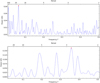 |
Fig. B.1. GLS periodogram of 6 GHz Stokes I data set (upper panel) and 33 GHz Stokes I data set (lower panel). Period is given in minutes. The red circles indicate the maximum peak found in the data: 15.7 ± 0.3 minutes at 6 GHz and 2.79 ± 0.05 minutes at 33 GHz. |
All Tables
All Figures
|
Fig. 1. VLA observations of the central binary VHS 1256−1257 AB. The size of the radio beam is shown in the lower left corner of each panel. Upper panel: Stokes I image of the 6 GHz data set. Lower panel: same as upper panel, but for the 33 GHz data set. |
| In the text | |
|
Fig. 2. Time evolution of flux density in VHS 1256−1257 at 6 GHz. Upper panel: points show the total flux density (Stokes I) averaged every 60 s, with a mean value of 78 μJy (plotted as a dashed line) and with a standard deviation of 37 μJy (plotted as a gray shadow). Lower panel: same as upper panel, but for Stokes V. The mean and standard deviation values in this case are 4 μJy and 38 μJy, respectively. |
| In the text | |
|
Fig. 3. Same as Fig. 2, but for the VLA 33 GHz observations. Mean and standard deviation values are 49 and 58 μJy (Stokes I) and 7 and 89 μJy (Stokes V). |
| In the text | |
|
Fig. 4. Total flux density of VHS 1256−1257AB from VLA observations updated with our new data and with published data (Guirado et al. 2018) on a smaller bandwidth sampling (circles). Different colors indicate different bands: 1.4 GHz (red), 6 GHz (yellow), 10 GHz (green), 33 GHz (blue), 230 GHz, and 345 GHz (gray). 3σ non-detections are plotted as arrows. Lines represent different gyrosynchrotron models with δ = 1.36 (see Sect. 5.3.1): dotted line for localized emitting region at the stellar surface with size of 1 R* (LES1) and dashed and dash-dot lines for radiation belts with B0 = 2000 G (RB2) and B0 = 3000 G (RB3), respectively. |
| In the text | |
|
Fig. 5. Same as Fig. 4, but this time lines represent the different gyrosynchrotron models discussed in Sects. 5.3.2 and 5.3.3. Red and black dashed lines for radiation belts at LF with B0 = 2000 G and B0 = 3000 G, respectively; red and black dotted line for a localized emission at HF and radiation belts with B0 = 3000 G, respectively; red solid line for the combination of radiation belts with B0 = 2000 G at LF and B0 = 3000 G at HF; black solid line for the combination of radiation belts with B0 = 2000 G at LF and a localized region at HF. |
| In the text | |
|
Fig. B.1. GLS periodogram of 6 GHz Stokes I data set (upper panel) and 33 GHz Stokes I data set (lower panel). Period is given in minutes. The red circles indicate the maximum peak found in the data: 15.7 ± 0.3 minutes at 6 GHz and 2.79 ± 0.05 minutes at 33 GHz. |
| In the text | |
Current usage metrics show cumulative count of Article Views (full-text article views including HTML views, PDF and ePub downloads, according to the available data) and Abstracts Views on Vision4Press platform.
Data correspond to usage on the plateform after 2015. The current usage metrics is available 48-96 hours after online publication and is updated daily on week days.
Initial download of the metrics may take a while.