| Issue |
A&A
Volume 678, October 2023
|
|
|---|---|---|
| Article Number | A185 | |
| Number of page(s) | 6 | |
| Section | Stellar structure and evolution | |
| DOI | https://doi.org/10.1051/0004-6361/202347156 | |
| Published online | 20 October 2023 | |
Understanding the radio emission from ϵ Eridani
1
Instituto de Radioastronomía y Astrofísica, Universidad Nacional Autónoma de México, A.P. 3-72 (Xangari), 58089 Morelia, Michoacán, Mexico
e-mail: This email address is being protected from spambots. You need JavaScript enabled to view it.
2
Instituto de Astronomía, Universidad Nacional Autónoma de México, A.P. 70-264, CDMX 04510, Mexico
Received:
11
June
2023
Accepted:
28
August
2023
Abstract
Some solar-type stars are known to present faint, time-variable radio continuum emission whose nature is not clearly established. We report on Jansky Very Large Array observations of the nearby star ϵ Eridani at 10.0 and 33.0 GHz. We find that this star has flux density variations on scales down to days, hours, and minutes. On 2020 April 15 it exhibited a radio pulse at 10.0 GHz with a total duration of about 20 min and a peak four times larger than the plateau of 40 μJy present in that epoch. We were able to model the time behavior of this radio pulse in terms of the radiation from shocks ramming into the stellar wind. Such shocks can be produced by the wind interaction of violently expanding gas heated suddenly by energetic electrons from a stellar flare, similar to the observed solar flares. Because of the large temperature needed in the working surface to produce the observed emission, this has to be nonthermal. It could be gyrosynchrotron or synchrotron emission. Unfortunately, the spectral index or polarization measurements from the radio pulse do not have a high enough signal-to-noise ratio to allow us to determine its nature.
Key words: radiation mechanisms: general / stars: individual: ϵ Eridani / radio continuum: stars
© The Authors 2023
 Open Access article, published by EDP Sciences, under the terms of the Creative Commons Attribution License (https://creativecommons.org/licenses/by/4.0), which permits unrestricted use, distribution, and reproduction in any medium, provided the original work is properly cited.
This article is published in open access under the Subscribe to Open model. This email address is being protected from spambots. You need JavaScript enabled to view it. to support open access publication.
1. Introduction
Located at 3.22 pc, ϵ Eridani (HD 22049) is a young Sun-like star close to our Solar System. Its spectral type is K2V, and its estimated age is 0.8 Gyr (Di Folco et al. 2004). It has a circumstellar debris disk with a physical extension of ∼64 AU and a radial width of ∼20 AU, possibly the residual of the process of formation of a young planetary system (Greaves et al. 1998). Backman et al. (2009) and Reidemeister et al. (2011) have suggested that this disk consists of different components: two warm inner belts, a cold outer belt, and an extended halo of small grains. Observations by Chavez-Dagostino et al. (2016) and Bastian et al. (2018) show continuum emission from the central star at millimeter and centimeter wavelengths.
Like our Sun, ϵ Eridani exhibits an active chromosphere (e.g., Baliunas et al. 1981), as well as an active X-ray corona (e.g., Johnson 1981). In addition, it shows a magnetic activity cycle, which was originally reported by Hatzes et al. (2000). Metcalfe et al. (2013) report the simultaneous operation of two magnetic activity cycles, where the amplitude of the shorter cycle of 2.95 yr (see, also, Jeffers et al. 2017) is modulated by a longer, 12.7-year cycle. This resembles the interaction of the 11-year solar cycle with the quasi-biennial (2-year) variations of the Sun (Fletcher et al. 2010).
Bastian et al. (2018) observed radio-continuum emission associated with ϵ Eridani with the Jansky Very Large Array (VLA) at four frequency bands: 2–4 GHz, 4–8 GHz, 8–12 GHz, and 12–18 GHz. They report quasi-steady unpolarized emission in the three high-frequency bands, and point out that this quiescent emission is consistent with optically thick emission from the star at coronal temperatures. In the coronal regions of ϵ Eridani, the opacity at frequencies higher than 2–4 GHz is dominated by gyroresonance absorption, suggesting magnetic fields between 475 G and 2700 G in the low corona and the production of gyroresonance emission between 4–8 GHz and 8–12 GHz.
In addition, Bastian et al. (2018) detected a radio pulse from ϵ Eridani in the 2–4 GHz band. The detected radio pulse (a sudden brief increase in emission) had a degree of circular polarization of up to 50% and lasted a few minutes. They proposed that the origin of the radio pulse may be nonthermal gyrosynchrotron emission from mildly relativistic electrons interacting with the coronal magnetic fields (∼100 G) of the star. Alternatively, coherent cyclotron maser instability emission in the bandwidth 2–4 GHz is also a possible mechanism for the stellar conditions, with magnetic fields of 700–1400 kG. Nevertheless, the problem for cyclotron maser instability emission in coronal conditions is the escape of the radiation, since it is absorbed by gyroresonance processes. Alternatively, Bastian et al. (2018) discuss the possibility that the radio pulse could come from an as yet undetected nearby planet with a 1 kG magnetic field, from the interaction with space weather events driven by stellar flares and/or coronal mass ejections from ϵ Eridani.
Bastian et al. (1998) pointed out that radio observations were fundamental in establishing that particle acceleration in solar flares is a two-phase process (Wild et al. 1963). There is a first phase of particle acceleration in which electrons reach energies of ∼100 keV, producing hard X-ray emission, microwave emission, and type III radio bursts. A second phase occurs ∼10 min after the first phase, in which shock waves are produced by the initial energy released. These shocks then propagate into the corona. During the latter stage, electrons and ions are further accelerated by the Fermi mechanism to energies as high as 100 MeV and 1 GeV, respectively, and type II and type IV radio bursts occur. These bursts are thought to be responsible for geomagnetic effects. In addition, since their discovery, coronal mass ejections have been recognized as the primary drivers of interplanetary and geomagnetic perturbations (see Gosling et al. 1991; Gosling 1993). Consequently, an accepted point of view nowadays is that interplanetary and geomagnetic disturbances are produced by two types of solar energetic phenomena, flares and coronal mass ejections, whose relationship is still poorly understood.
Recently, Burton et al. (2022) reported the detection of three flares from ϵ Eridani using the Atacama Large Millimeter Array (ALMA) at 1.3 mm. They characterized the temporal, spectral, and polarization of these flare events and suggested that their properties are similar to those of the Sun at similar wavelengths. Also, Loyd et al. (2022) conducted a coronal dimming analysis at far-ultraviolet spectral lines in archival observations of ϵ Eridani and found a prominent flare in the 2015 data.
In another work, Rodriguez et al. (2019, hereafter RLL19) reported VLA observations of ϵ Eridani at 33 GHz. These observations had high enough angular resolution to demonstrate the stellar origin of the radio emission since the detected emission has an angular size of  (which corresponds to a physical extension of 0.2 au from the star), which is smaller than the semimajor axis (∼3.4 au) of the exoplanet ϵ Eridani b. In addition, RLL19 showed that the observed centimeter emission of ϵ Eridani from 5 to 50 GHz is remarkably flat and could be due to optically thin free–free emission from a steady stellar wind with a mass-loss rate of ∼6.6 × 10⁻¹¹ M⊙ yr−1, which is 3300 times larger than the solar value, Ṁ⊙ = 2 × 10⁻¹⁴ M⊙ yr−1 (Feldman et al. 1977). Nonetheless, other mechanisms such as coronal free–free and gyroresonance emission could not be ruled out. The high mass-loss rate inferred by RLL19 is at odds with the mass-loss rate 30 times the solar value estimated by Wood et al. (2002) from the interstellar hot HI that surrounds the star and is observed in absorption in the Lyα spectrum. The Lyα absorption comes from the interstellar medium gas that is heated by the interaction with the stellar wind. Wood et al. (2002) used hydrodynamic models of astrospheres to infer the mass-loss rates from the HI absorption. Furthermore, Cranmer & Saar (2011) modeled the steady mass-loss rates of cool main-sequence stars and evolved giants. They studied magnetohydrodynamic turbulence motions from subsurface convection zones and their dissipation and escape through the stellar wind. They estimated an even smaller value for the mass-loss rate of ϵ Eridani, of only 2.4 times the solar value. On the other hand, Johnstone et al. (2015) investigated the evolution of stellar rotation and wind properties of low-mass main-sequence stars. They note that there is a large uncertainty regarding the evolution of the stellar winds of these stars, the major problems being the lack of observational constraints on the wind properties and the large spread in rotation rates at young ages. Thus, disagreement between the mass-loss rates obtained from observations and theoretical models of ϵ Eridani is still an open problem.
One way to determine if the observed radio emission from ϵ Eridani is thermal or nonthermal is to study the variability and/or polarization characteristics of the emission. Extremely fast variability would imply that the source is small, and very high brightness temperatures, not achievable with thermal mechanisms, would be required. The presence of linear or circular polarization is indicative of synchrotron or gyrosynchrotron emission, respectively (Güdel 2002). In addition, the spectral index could help in determining the nature of the radio emission, since negative indices (< − 0.1) cannot be obtained with free–free emission (Rodriguez et al. 1993). For this reason, we monitored the source at 10 GHz and 33 GHz, notably finding a radio pulse at 10 GHz. We investigated the possibility that the pulse can be produced by shocks in the ϵ Eridani stellar wind. As discussed above, such shocks could be produced in the second phase of stellar flares, after the magnetic energy is released.
The rest of this paper is organized as follows. In Sects. 2 and 3 we discuss the observations. In Sect. 4 we present the model of the flare–wind interaction used to interpret the radio pulse observed at 10 GHz. In Sect. 5 we present our conclusions.
2. Observations
The observations were part of our VLA project 20A-020, made with the Karl G. Jansky VLA of NRAO1 in its C configuration during eight epochs in 2020 February–May. We used the X band (8–12 GHz) at six epochs and the Ka band (29–37 GHz) at two epochs. The flux and bandpass calibrator was J0137+3309 or J0542+4951, and the phase calibrator was always J0339−0146. In the X band, the digital correlator of the VLA was configured in 32 spectral windows of 128 MHz width, covering the range 8–12 GHz. In the Ka band, the digital correlator of the VLA was configured in 64 spectral windows of 128 MHz width, covering the range 29–37 GHz. In both bands, each spectral window is divided into 64 channels with an individual spectral resolution of 2 MHz. The data were calibrated in the standard manner using the Common Astronomy Software Applications (CASA) package of NRAO and the pipeline provided for VLA2 observations (McMullin et al. 2007).
We created an image concatenating the six epochs observed at 10.0 GHz (the center of the X band) to search for sources in the field. A robust weighting of 2 (Briggs 1995) was used to optimize sensitivity in all the images discussed here. A total of 13 sources were detected (see Table 1). One of the radio sources corresponds to ϵ Eridani and of the remaining 12 sources, 10 had been previously detected by RLL19. With the exception of [RLL2019] 3, which shows an increase of a factor of 2 between the observations reported in RLL19 (taken in 2013) and those presented here, the other sources show flux densities consistent within ∼25% between the two epochs.
10 GHz sources in the field of ϵ Eridani.
The region was observed at 10.0 GHz at six epochs and at 33.0 GHz (the center of the Ka band) at two epochs, as listed in Table 2. In this table we also give the flux densities of ϵ Eridani and of the steady source [RLL2019] 7 for each individual epoch. [RLL2019] 7 was used as a comparison source to check that the variability was not due to some systematic effect. While [RLL2019] 7 shows 10.0 GHz flux densities that, within the noise, are consistent with no variability, ϵ Eridani exhibits important time variability. Two observations made on 2020 April 05 at 10.0 GHz with a time difference of 3.6 h show a flux density increase of about 2.2. On 2020 April 15, ϵ Eridani appeared unusually bright. A 10 GHz image of the emission at that epoch is shown in Fig. 1. An analysis of the flux density within the time interval of the observations (approximately one hour) shows that most of the increase comes from a flare. This flare had a duration of only about 20 min and shows the characteristic rapid rise and slower fall of flares (see Fig. 2). We tried to estimate the spectral index of the emission during the flare by making images at 9.0 and 11.0 GHz. The flux densities obtained, 155±17 and 175±24 μJy respectively, imply a spectral index of 0.6±0.9, which, unfortunately, does not have a high enough signal-to-noise ratio to discriminate between possible emission mechanisms. The poor signal-to-noise ratio comes from the fact that the two frequencies used are close to each other.
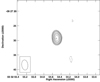 |
Fig. 1. 10.0 GHz image of ϵ Eridani for the epoch 2020 April 15. Contours are −4, −3, 3, 4, 5, 6, 8, 10, 12, and 15 times 4.0 μJy beam−1, the rms noise in this region of the image. The synthesized beam ( |

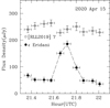 |
Fig. 2. 10.0 GHz flux densities for ϵ Eridani (solid circles) and [RLL2019] 7 (hollow squares) during the observations of 2020 April 15. The hour is given in Coordinated Universal Time (UTC). The horizontal bars indicate the duration of the scan, while the vertical bars indicate the noise of the measurement. The dashed line joins the data points for ϵ Eridani. We have added 80 μJy to the flux densities of [RLL2019] 7 to better separate the data points of the two sources. |
Flux density of ϵ Eridani and [RLL2019] 7 as a function of time (averaged over each epoch of observation).
At 33 GHz, ϵ Eridani was detected only in the observations of 2020 May 08. Given the small primary beam and lower sensitivity at this frequency, this was the only source detected. Between the two epochs observed at 33 GHz, with a separation of 10 days, the flux density decreased by a factor of at least ∼2. Again, we tried to estimate the spectral index of the emission on 2020 May 08 by making images at 31.0 and 35.0 GHz. The flux densities obtained, 62±15 and 61±20 μJy respectively, imply a spectral index of −0.1±3.4, which, again, does not have a high enough signal-to-noise ratio to discriminate between possible emission mechanisms. Finally, the last column of Table 2 gives the 4σ upper limit to the circular polarization of ϵ Eridani. No circular polarization was detected at any epoch.
3. Individual sources
3.1. Sources 2 and 13
As noted by RLL19, source 11 of Table 1 is associated with a millimeter source detected by Chavez-Dagostino et al. (2016). In the  region we imaged at 10.0 GHz, a total of 13 radio sources were detected (Table 1). We wanted to include optical counterparts other than ϵ Eri and thus added the Gaia Data Release 3 sources from the same region of the sky to our sample (Gaia Collaboration 2016, 2023), for a total of 64 sources. Remarkably, radio sources 2 and 13 coincide within
  with the sources Gaia DR3 5164707626664526592 and 5164696081792414464, respectively. We speculate that these two Gaia sources could be background galaxies. According to the NASA/IPAC Extragalactic Database (NED), only source 2 is an infrared source. However, there are no other data, and the nature of the source (galactic or extragalactic) is not determined in the NED.
3.2. Source 11
This source was detected as a single source in the 2013 observations presented by RLL19, which had an angular resolution of ∼6″. The higher-angular-resolution observations presented here (Fig. 3) show it is actually a double source, probably a radio galaxy.
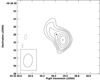 |
Fig. 3. 10.0 GHz image of the VLA11 region from all the data obtained in 2020. Contours are −4, −3, 3, 4, 5, 6, 8, 10, and 12 times 2.4 μJy beam−1, the rms noise in this region of the image. The synthesized beam ( |

4. The radio behavior of ϵ Eridani
4.1. Comparison with the Sun
At 10.0 GHz, the quiet Sun (at sunspot minimum) has a flux density of ≃2.8 × 10⁶ Jy as measured from the Earth (Giersch & Kennewell 2022). A typical plateau flux density for ϵ Eridani at 10.0 GHz is ≃40 μJy (this paper). If it were located at 1 au, we would measure a flux density of ≃1.8 × 10⁷ Jy, about eight times larger than that of the Sun.
With respect to flare activity, Nita et al. (2002) investigated the peak flux distribution of 40 years of solar radio burst data. They find that in the 8.4–11.8 GHz band during solar maximum, one can expect one flare above 8 × 10⁷ Jy about every 30 days. The total peak flux density of 190 μJy of the ϵ Eridani flare reported here would become 8.4 × 10⁷ Jy at 1 au, comparable to the brightest solar flares. On the other hand, Wang et al. (2020) studied 86 solar events at 9.4 GHz between 2000 and 2010. They find that the peak flux densities are distributed along two orders of magnitude, from about 2 × 10⁵ to about 2 × 10⁷ Jy, but the relatively small number of flares observed limits their statistics.
4.2. Interpretation of the observed radio pulse at 10 GHz
Unfortunately, it was not possible to determine the spectral index of the emission during the radio pulse at 10 GHz accurately enough to determine if the origin of the emission is thermal or nonthermal. As discussed in Sect. 4.2, the derived value of the spectral index is 0.6±0.9.
The observed pulse at 10 GHz could be produced by shocks in the ionized stellar wind of ϵ Eridani (see RLL19). As mentioned above, shocks can occur from the interaction of gas heated by energetic electrons from a stellar flare with the steady stellar wind of the star. When the heated gas collides with the stellar wind, a working surface (WS), bounded by two shock fronts, will be formed as a fast flow overtakes the previously ejected slow wind. In this section we model the observed radio pulse at 10 GHz of ϵ Eridani as produced by shocks in the stellar wind inside a cone with solid angle Ω.
We assumed that there is an increase in the flow velocity at the base of the wind, that is, during the violent expansion event the ejection velocity drastically increases with respect to the stellar wind value. We also allowed the expanding gas to have a mass-loss rate different from that of the stellar wind. This type of variability in the flow parameters has previously been studied by Montes-Doria et al. (2022) in the case of the Sun. They used the general model of the WS dynamics from Cantó et al. (2000) for highly supersonic flows, which is based on mass and momentum conservation.
The Montes-Doria et al. (2022) model gives an analytic solution for the dynamical evolution of the WS. In this model, the wind is ejected with a constant velocity v1 = vw and an isotropic mass-loss rate Ṁw. At an injection time τ = 0, one considers mass injection within a solid angle Ω, with an increased velocity v2 = a v1, with a > 1, during an interval of time Δτ, and a change in the mass-loss rate per unit solid angle from the wind mass-loss rate ṁ1 = Ṁw/4π to ṁ2 = bṁ1. In this case, the WS forms instantaneously and has an initial phase where it moves at a constant speed, vWS = σvw, where σ = a1/2(1 + a1/2b1/2)/(a1/2 + b1/2). Consequently, the position of the WS during this initial phase is given by rWS = R* + σvwt, where R* is the injection radius. Once all the heated gas has entered the WS, the inner shock disappears, giving rise to a decelerating phase. This occurs at a critical time tc = a Δτ/(a − σ). For later times, the WS decelerates with a velocity and position given by Eqs. (2) and (3) of Montes-Doria et al. (2022). The WS moves away from the source and decelerates, asymptotically approaching the wind velocity, vw. During its evolution, the WS will lose energy via radiation. From Eqs. (4), (5), and (19) of Cantó et al. (2000), the bolometric luminosity of the WS (within the solid angle Ω) can be written as
 (1)
(1)
for t ≤ tc, when the WS is bounded by two shocks, and
 (2)
(2)
for t > tc, when the internal shock disappears and the WS decelerates.
For simplicity, we assumed that a constant fraction, ϵ, of the WS bolometric luminosity is radiated at 10 GHz. Thus, the 10 GHz flux is given by
 (3)
(3)
where FWS is the bolometric flux, and D = 3.22 pc is the distance to ϵ Eridani.
To correct the ten data points of the 2020 April 15 observations, we fitted and subtracted the slope of a baseline in time obtained from a linear fit to the first four points. The resulting flux densities are given in Table 3. In Fig. 4 we show these data points as well as a model, as a solid red line. This model gives the flux from a WS produced in a wind with mass-loss rate Ṁw = 6.6 × 10⁻¹¹ M⊙ yr−1 and velocity vw = 650 km s−1 (taken from the model of RLL2019 for the steady wind of ϵ Eridani), a velocity increase a = 3.3, a mass-loss rate parameter b = 2.6, a time interval of injection of high velocity gas Δτ = 3.0 min, and a solid angle Ω = 9.5 × 10⁻² str (corresponding to a half opening angle θ = 10°). The emission of the WS is superimposed on a steady wind emission of 40 μJy. The WS has initial velocity vWS = 1300 km s−1. The inner shock disappears at the critical time tc = 8.2 min, and then the WS starts to decelerate and eventually reaches the wind velocity. The deceleration starts at a distance Rc = 1.7 R⊙ from the center of the star. We note that the duration of the observed radio pulse is longer than the model time interval of ejection of fast material (Δτ).
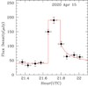 |
Fig. 4. Model of the radio pulse as the emission of a WS formed in the stellar wind (solid red line) superimposed on a steady emission of 40 μJy. The data points are those given in Table 3. |
Flux density of ϵ Eridani at 10 GHz on 2020 April 15.
The observed maximum flux of the radio pulse is 150 μJy, emitted on top of a steady wind emission of 40 μJy. For the shock model discussed above, the maximum of the total bolometric flux is Fmax = 1.4 × 10¹³ Jy (obtained by substituting vWS/vw = σ in Eqs. (1) and (3)). To observe 150 μJy at the peak of the 10 GHz pulse, one needs a fraction, ϵ, of the total energy emitted at this frequency to be ϵ = 150 μJy/Fmax = 1.0 × 10⁻¹⁷. On the other hand, as discussed in the Introduction, Wood et al. (2002) estimated a mass-loss rate for ϵ Eridani of 30 times the solar value, that is to say, 110 times smaller than the value of RLL19. Assuming the same wind speed (which is the escape speed from the surface of the star), the shock would have a maximum flux, Fmax, 110 times smaller because the shock luminosity is proportional to Ṁw (Eq. (1)). In this case, the fraction of the total energy emitted at 10 GHz would be 110 times higher, namely ϵ = 1.2 × 10⁻¹⁵.
In this simple model, we do not solve for the shock microphysics. Nevertheless, it can be used to obtain further insights into the origin of the emission. First, the estimated size, l, of the emitting region at the distance Rc = 1.7 R⊙ with opening angle θ = 10° is l ∼ 2.1 × 1010 cm. Thus, at the distance of ϵ Eridani, the WS would need to have a brightness temperature Tb ∼ 3.6 × 10⁶ K to produce the observed peak flux of 150 μJy at 10 GHz.
If the emission is thermal, one can calculate the fraction of energy emitted by a black body (BB) in the range 8–12 GHz. The integral over the whole spectrum, Bν(T), is  , where σB is the Stefan-Boltzmann constant. In the Rayleigh-Jeans approximation, the integral over the VLA bandwidth at 10 GHz is
  . Then, the fraction of the BB energy that is radiated in the 10 GHz band is ϵBB = I10 GHz/Itotal = 1.4 × 10⁻²²(T/3.6×106 K)−3. The fraction of thermal BB energy emitted at 10 GHz is thus too small compared to the values calculated above and so the emission of the WS cannot be thermal emission. Therefore, the emission produced by the WS needs to be nonthermal, for example synchrotron emission by relativistic electrons accelerated in the shocks via the Fermi mechanism. In the Sun after a solar flare, electrons are Fermi-accelerated in shocks up to energies of 100 Mev (e.g., Bastian et al. 1998).
In summary, internal shocks produced in the wind, expected from gas heated by stellar flares, can produce the temporal variation in the observed 10 GHz pulse in ϵ Eridani. The emission of the WS has to be nonthermal. Further monitoring of this source is needed to obtain the spectral index or polarization measurements of the radio emission and thus further constrain the emission mechanism. The nonthermal emission could be due to gyrosynchrotron from a flare due to magnetic reconnection in the low corona (Nita et al. 2002) or to synchrotron emission from relativistic electrons accelerated in shocks, as in the scenario discussed above. Further observations are required to determine the polarization state and spectral index of the emission. A positive spectral index would indicate gyrosynchrotron or optically thick synchrotron emission. In addition, gyrosynchrotron would produce circularly polarized emission, while one expects linear polarization in the case of synchrotron emission (Güdel 2002). In particular, the observed radiation is entirely consistent with nonthermal gyrosynchrotron emission from a solar-like flare in the low corona. For example, for a source radius of 5% of the stellar radius, the brightness temperature would be a few times 108 K, consistent with nonthermal gyrosynchrotron emission. This interpretation is also supported by the fact that at lower frequencies Bastian et al. (2018) doubtless detected a gyrosynchrotron pulse.
5. Conclusions
Our main conclusions can be summarized as follows:
We present sensitive, high-angular-resolution VLA observations of the nearby (3.22 pc) Sun-like star epsilon Eridani at 10.0 (six epochs) and 33.0 GHz (two epochs). While the other radio sources in the field are steady, ϵ Eridani shows flux density variations down to scales of days, hours, and even minutes. The emission at 10 GHz, excluding the radio pulse observed on 2020 April 15, varied by a factor of ∼3 during the observation campaign.
The 2020 April 15 radio pulse of ϵ Eridani lasted for about 20 min. At the peak of the pulse, the flux density was ∼150 μJy, a factor of ∼4 above the plateau of ∼40 μJy present at that epoch.
We successfully modeled the energy and temporal variation in the 10 GHz radio pulse in terms of the emission from shocks in the wind of ϵ Eridani. These shocks have enough energy to produce the observed flux. The model does not solve for the microphysics of the shock emission. Nevertheless, the brightness temperature required to produce the observed flux implies that the emission has to be nonthermal.
Unfortunately, neither the spectral index nor the polarization measurements of the radio flare emission are stringent enough to determine the nature of the nonthermal radio emission, either gyrosynchrotron from stellar flares or synchrotron emission from relativistic electrons accelerated in shocks. However, the observed flare radiation is consistent with nonthermal gyrosynchrotron emission from a solar-like flare in the low corona. Ultra-sensitive observations such as those that will be provided by the Square Kilometer Array and the Next Generation VLA may be required to firmly establish the nature of the radio emission of ϵ Eridani and similar stars.
The National Radio Astronomy Observatory is a facility of the National Science Foundation operated under cooperative agreement by Associated Universities, Inc.
Acknowledgments
This work was supported by grants PAPIIT-UNAM IN103921, IG100422, IN103023. This research has made use of the NASA/IPAC Extragalactic Database (NED), which is funded by the National Aeronautics and Space Administration and operated by the California Institute of Technology. This work has made use of data from the European Space Agency (ESA) mission Gaia (https://www.cosmos.esa.int/gaia), processed by the Gaia Data Processing and Analysis Consortium (DPAC, https://www.cosmos.esa.int/web/gaia/dpac/consortium). Funding for the DPAC has been provided by national institutions, in particular the institutions participating in the Gaia Multilateral Agreement. We thank the referee for very useful comments that improved the interpretation of the data.
References
- Backman, D., Marengo, M., Stapelfeldt, K., et al. 2009, ApJ, 690, 1522 [Google Scholar]
- Baliunas, S. L., Hartmann, L., Vaughan, A. H., et al. 1981, ApJ, 246, 473 [NASA ADS] [CrossRef] [Google Scholar]
- Bastian, T. S., Benz, A. O., & Gary, D. E. 1998, ARA&A, 36, 131 [Google Scholar]
- Bastian, T. S., Villadsen, J., Maps, A., et al. 2018, ApJ, 857, 133 [NASA ADS] [CrossRef] [Google Scholar]
- Benedict, G. F., McArthur, B. E., Gatewood, G., et al. 2006, AJ, 132, 2206 [Google Scholar]
- Briggs, D. S. 1995, Bull. Am. Astron. Soc., 27, 1444 [Google Scholar]
- Burton, K., MacGregor, M. A., & Osten, R. A. 2022, ApJ, 939, L6 [CrossRef] [Google Scholar]
- Cantó, J., Raga, A. C., & D’Alessio, P. 2000, MNRAS, 313, 656 [CrossRef] [Google Scholar]
- Chavez-Dagostino, M., Bertone, E., Cruz-Saenz Miera, F., et al. 2016, MNRAS, 462, 2285 [NASA ADS] [CrossRef] [Google Scholar]
- Cranmer, S. R., & Saar, S. H. 2011, ApJ, 741, 54 [Google Scholar]
- Di Folco, E., Thévenin, F., Kervella, P., et al. 2004, A&A, 426, 601 [NASA ADS] [CrossRef] [EDP Sciences] [Google Scholar]
- Feldman, W. C., Asbridge, J. R., Bame, S. J., et al. 1977, The Solar Output and its Variation, 351 [Google Scholar]
- Fletcher, S. T., Broomhall, A.-M., Salabert, D., et al. 2010, ApJ, 718, L19 [NASA ADS] [CrossRef] [Google Scholar]
- Gaia Collaboration (Prusti, T., et al.) 2016, A&A, 595, A1 [NASA ADS] [CrossRef] [EDP Sciences] [Google Scholar]
- Gaia Collaboration (Brown, A. G. A., et al.) 2020, VizieR Online Data Catalog: I/350 [Google Scholar]
- Gaia Collaboration (Vallenari, A., et al.) 2023, A&A, 674, A1 [NASA ADS] [CrossRef] [EDP Sciences] [Google Scholar]
- Giersch, O., & Kennewell, J. 2022, Radio Sci., 57, e2022RS007456 [NASA ADS] [CrossRef] [Google Scholar]
- Gosling, J. T. 1993, J. Geophys. Res., 98, 18937 [NASA ADS] [CrossRef] [Google Scholar]
- Gosling, J. T., McComas, D. J., Phillips, J. L., et al. 1991, J. Geophys. Res., 96, 7831 [NASA ADS] [CrossRef] [Google Scholar]
- Greaves, J. S., Holland, W. S., Moriarty-Schieven, G., et al. 1998, ApJ, 506, L133 [NASA ADS] [CrossRef] [Google Scholar]
- Güdel, M. 2002, ARA&A, 40, 217 [Google Scholar]
- Hatzes, A. P., Cochran, W. D., McArthur, B., et al. 2000, ApJ, 544, L145 [Google Scholar]
- Jeffers, S. V., Boro Saikia, S., Barnes, J. R., et al. 2017, MNRAS, 471, L96 [NASA ADS] [Google Scholar]
- Johnson, H. M. 1981, ApJ, 243, 234 [NASA ADS] [CrossRef] [Google Scholar]
- Johnstone, C. P., Güdel, M., Brott, I., et al. 2015, A&A, 577, A28 [NASA ADS] [CrossRef] [EDP Sciences] [Google Scholar]
- Loyd, R. O. P., Mason, J. P., Jin, M., et al. 2022, ApJ, 936, 170 [NASA ADS] [CrossRef] [Google Scholar]
- McMullin, J. P., Waters, B., Schiebel, D., et al. 2007, ASP Conf. Ser., 376, 127 [NASA ADS] [Google Scholar]
- Metcalfe, T. S., Buccino, A. P., Brown, B. P., et al. 2013, ApJ, 763, L26 [Google Scholar]
- Montes-Doria, D., González, R. F., Cantó, J., et al. 2022, MNRAS, 509, 1892 [Google Scholar]
- Nita, G. M., Gary, D. E., Lanzerotti, L. J., et al. 2002, ApJ, 570, 423 [CrossRef] [Google Scholar]
- Reidemeister, M., Krivov, A. V., Stark, C. C., et al. 2011, A&A, 527, A57 [NASA ADS] [CrossRef] [EDP Sciences] [Google Scholar]
- Rodriguez, L. F., Marti, J., Canto, J., et al. 1993, Rev. Mex. Astron. Astrofis., 25, 2 [Google Scholar]
- Rodriguez, L. F., Lizano, S., Loinard, L., et al. 2019, ApJ, 871, 172 [CrossRef] [Google Scholar]
- Wang, L., Liu, S.-M., & Ning, Z.-J. 2020, RAA, 20, 178 [NASA ADS] [Google Scholar]
- Wild, J. P., Smerd, S. F., & Weiss, A. A. 1963, ARA&A, 1, 291 [NASA ADS] [CrossRef] [Google Scholar]
- Wood, B. E., Müller, H.-R., Zank, G. P., et al. 2002, ApJ, 574, 412 [NASA ADS] [CrossRef] [Google Scholar]
All Tables
Flux density of ϵ Eridani and [RLL2019] 7 as a function of time (averaged over each epoch of observation).
All Figures
|
Fig. 1. 10.0 GHz image of ϵ Eridani for the epoch 2020 April 15. Contours are −4, −3, 3, 4, 5, 6, 8, 10, 12, and 15 times 4.0 μJy beam−1, the rms noise in this region of the image. The synthesized beam ( |
| In the text | |
|
Fig. 2. 10.0 GHz flux densities for ϵ Eridani (solid circles) and [RLL2019] 7 (hollow squares) during the observations of 2020 April 15. The hour is given in Coordinated Universal Time (UTC). The horizontal bars indicate the duration of the scan, while the vertical bars indicate the noise of the measurement. The dashed line joins the data points for ϵ Eridani. We have added 80 μJy to the flux densities of [RLL2019] 7 to better separate the data points of the two sources. |
| In the text | |
|
Fig. 3. 10.0 GHz image of the VLA11 region from all the data obtained in 2020. Contours are −4, −3, 3, 4, 5, 6, 8, 10, and 12 times 2.4 μJy beam−1, the rms noise in this region of the image. The synthesized beam ( |
| In the text | |
|
Fig. 4. Model of the radio pulse as the emission of a WS formed in the stellar wind (solid red line) superimposed on a steady emission of 40 μJy. The data points are those given in Table 3. |
| In the text | |
Current usage metrics show cumulative count of Article Views (full-text article views including HTML views, PDF and ePub downloads, according to the available data) and Abstracts Views on Vision4Press platform.
Data correspond to usage on the plateform after 2015. The current usage metrics is available 48-96 hours after online publication and is updated daily on week days.
Initial download of the metrics may take a while.