| Issue |
A&A
Volume 660, April 2022
|
|
|---|---|---|
| Article Number | A71 | |
| Number of page(s) | 8 | |
| Section | The Sun and the Heliosphere | |
| DOI | https://doi.org/10.1051/0004-6361/202142201 | |
| Published online | 13 April 2022 | |
Excitation of Langmuir waves at shocks and solar type II radio bursts
1
Leibniz-Institut für Astrophysik Potsdam (AIP), An der Sternwarte 16, 14482 Potsdam, Germany
e-mail: This email address is being protected from spambots. You need JavaScript enabled to view it.
2
Solar-Terrestrial Centre of Excellence – SIDC, Royal Observatory of Belgium, Avenue Circulaire 3, 1180 Brussels, Belgium
3
Centre for Mathematical Plasma Astrophysics, Department of Mathematics, KU Leuven, Celestijnenlaan 200B, 3001 Leuven, Belgium
4
CRAL Space, United Kingdom Research and Innovation (UKRI), Science & Technology Facilities Council (STFC), Rutherford Appleton Laboratory (RAL), Harwell Campus, Oxfordshire OX11 0QX, UK
5
Astronomy & Astrophysics Section, Dublin Institute for Advanced Studies, Dublin 2 D02 XF86, Ireland
6
Space Radio-Diagonostics Research Center, University of Warmia and Mazury, Oczapowskiego 2, 10-719 Olstyn, Poland
7
CBK PAN, Bartycka 18A, Warsaw 00-716, Poland
8
Institute for Radio Astronomy, Oude Hoogeveensedijk 4, 7991 PD Dwingeloo, The Netherlands
Received:
10
September
2021
Accepted:
10
January
2022
Abstract
Context. In the solar corona, shocks can be generated due to the pressure pulse of a flare and/or driven by a rising coronal mass ejection (CME). Coronal shock waves can be observed as solar type II radio bursts in the Sun’s radio radiation. In dynamic radio spectra, they appear as stripes of an enhanced radio emission slowly drifting from high to low frequencies. The radio emission is thought to be plasma emission, that is to say the emission happens near the electron plasma frequency and/or its harmonics. Plasma emission means that energetic electrons excite Langmuir waves, which convert into radio waves via non-linear plasma processes. Thus, energetic electrons are necessary for plasma emission. In the case of type II radio bursts, the energetic electrons are considered to be shock accelerated.
Aims. Shock drift acceleration (SDA) is regarded as the mechanism for producing energetic electrons in the foreshock region. SDA delivers a shifted loss-cone velocity distribution function (VDF) for the energetic electrons. The aim of the paper is to study in which way and under which conditions a shifted loss-cone VDF of electrons excites Langmuir waves in an efficient way in the corona.
Methods. By means of the results of SDA, the shape of the resulted VDF was derived. It is a shifted loss-cone VDF showing both a loss-cone and a beam-like component. The growth rates for exciting Langmuir waves were calculated in the framework of Maxwell-Vlasov equations. The results are discussed by employing plasma and shock parameters usually found in the corona at the 25 MHz level.
Results. We have found that moderate coronal shocks with an Alfven-Mach number in the range 1.59 < MA < 2.53 are able to accelerate electrons up to energies sufficient enough to excite Langmur waves, which convert into radio waves seen as solar type II radio bursts.
Key words: Sun: flares / Sun: radio radiation / Sun: particle emission / Sun: corona
© ESO 2022
1. Introduction
In astrophysics, shock waves play an important role since they are regarded as the source of cosmic rays. For instance, such shocks appear in the vicinity of super-nova remnants (see e.g. Dickel 1991), travelling interplanetary shocks ahead of coronal mass ejections (CMEs) (Uchida 1960; Stewart et al. 1974a,b; Hundhausen et al. 1984; Krimigis 1992), and bow shocks in the vicinity of planets (Krimigis 1992; Klassen et al. 2008) as well as in the solar corona (Uchida 1960; Stewart et al. 1974a,b; Rouillard et al. 2016). In the corona, shock waves can either be generated by blast waves due to pressure pulses of the flare (Uchida et al. 1973; Vršnak et al. 1995; Temmer et al. 2009; Magdalenic et al. 2012) or they can be driven by a CME (Stewart et al. 1974a,b; Hundhausen et al. 1984; Gopalswamy 2006; Melnik et al. 2008). Furthermore, coronal shock waves can also occur as so-called termination shocks in the outflow region of the magnetic reconnection region (Forbes 1986; Shibata et al. 1995; Aurass et al. 2002; Aurass & Mann 2004; Mann et al. 2009; Shen et al. 2018; Cai et al. 2019). Coronal shock waves can be observed as type II radio bursts in the metric and decameter wave ranges (Wild & McCready 1950; Uchida 1960; Cane et al. 1987; Melnik et al. 2004; Gopalswamy et al. 2005; Schmidt & Cairns 2012a,b; Schmidt et al. 2014; Zucca et al. 2018; Rouillard et al. 2016; Magdalenic et al. 2020; Kouloumvakos et al. 2021; Wu et al. 2021; see as reviews: Nelson & Melrose 1985; Mann 1995, 2006; Aurass 1996; Cairns et al. 2003).
An example of a solar type II radio burst is presented in Fig. 1 (adapted from Magdalenic et al. 2020). It was observed with the novel radio telescope LOFAR (LOw Frequency ARray) (van Haarlem et al. 2013) in the frequency range 10−90 MHz. This example shows all typical features of solar type II radio bursts (Smerd et al. 1962; Wild & Smerd 1972, see as reviews e.g. Nelson & Melrose 1985; Mann 1995). In dynamic radio spectra, type II bursts appear as stripes of enhanced radio emission. These stripes drift slowly from high to low frequencies. As in the presented example, type II bursts show a fundamental harmonic structure, that is at 15:15:00 UT the fundamental and harmonic band start at ≈30 and 60 MHz, respectively. The fundamental band drifts from 40 MHz to 14 MHz in the period 15:09−15:21 UT, leading to a drift rate of the fundamental band of −0.036 MHz s−1. It is a typical value in this frequency range (Mann 1995; Dorovskyy et al. 2015). Both the fundamental band and the harmonic one are divided into sub-bands. This is called band-splitting, which is a usual phenomenon of solar type II radio bursts (Smerd et al. 1962; Vršnak et al. 2001, 2002; Magdalenic et al. 2020). Furthermore, rapidly drifting stripes of enhanced radio emission are seen as fine structures in both the fundamental and harmonic band. They have typical drift rates of about ±1 MHz s−1 (Mann & Klassen 2005). They are called ‘herringbones’ (Nelson & Melrose 1985; Cairns & Robinson 1987; Mann et al. 2018) and are regarded as radio signatures of electron beams accelerated at the shock wave associated with the type II burst.
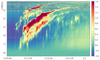 |
Fig. 1. Dynamic radio spectrum in the frequency range 10−90 MHz as recorded with the radio telescope LOFAR during the period 15:10−15:30 UT on 25 August 2014 The intensity is colour coded in arbitrary units as seen in the bar on the right-hand side (adapted from Magdalenic et al. 2020). |
In LOFAR’s frequency range, that is 10−240 MHz, the Sun’s non-thermal radio emission is thought to be plasma emission as originally proposed by Ginzburg & Zheleznyakov (1958). In this case, energetic electrons excite electrostatic Langmuir waves which convert into escaping radio waves due to non-linear plasma processes (Ginzburg & Zheleznyakov 1958; Melrose 1985 as a textbook). Thus, the radio waves are emitted near the local electron plasma frequency and/or its harmonics. As a result, the appearance of energetic electrons is a necessary requirement for exciting Langmuir waves and non-thermal radio emission.
Assuming plasma emission for type II radio bursts, the individual frequencies are emitted at different height levels because the electron plasma frequency depends on the square root of the electron number density and the density is gravitationally stratified in the corona. Hence, the up- and downward movement of a radio source manifests in a negative and positive drift in the dynamic radio spectrum, respectively. The density model by Mann et al. (1999) results from a special solution of Parker (1958) wind equation and describes the radial behaviour of the electron number density well from the corona up to 1 AU in the interplanetary space. It gives a relationship between the emission frequency and its radial localization in the corona.
In the special example presented in Fig. 1, the fundamental band drifts from 40 MHz to 14 MHz within 720 s. According to the density model of Mann et al. (1999), the 40 MHz and 14 MHz level correspond to a radial distance 2.25 R⊙ = 1.57 × 10⁶ km (R⊙, Sun’s radius) and 1.68 R⊙ = 1.17 × 10⁶ km, respectively. Thus, the shock travels a radial distance of 4.00 × 10⁵ km within 720 s resulting in a radial velocity of 556 km s−1.1 We note that this is the radial shock velocity. The real one can be much larger in the case of the shock travelling horizontally along the solar surface. The herringbones shooting away from both the fundamental and harmonic band towards higher and lower frequencies have drift rates of ±1.0 MHz s−1 in the example presented in Fig. 1, which is typical for these features (Mann & Klassen 2002; Dorovskyy et al. 2015). Such a drift rate results in a radial velocity of 25 000 km s−1 which should be regarded as a typical velocity of shock-accelerated electron beams in the corona (Mann & Klassen 2005). However, there are also cases in which the electrons associated with the herringbones have velocities up to 100 000 km s−1 as reported by Dorovskyy et al. (2015).
The type II burst presented in Fig. 1 appears around 25 MHz in the fundamental band. The 25 MHz level corresponding to an electron number density Ne = 7.75 × 106 cm−3 is typically located at a distance of ≈2 R⊙ from the centre of the Sun (Mann et al. 1999). At this height, a magnetic field B of 0.5 G (Dulk & McLean 1978) is obtained. The model by Dulk & McLean (1978) approximately describes the radial behaviour of the magnetic field strength above active regions, where solar type II radio bursts occur. With these parameters, one gets an electron plasma frequency ωpe = (4πe2Ne/me)1/2 = 1.57 × 10⁸ s−1 (e, elementary charge; me, electron mass), electron cyclotron frequency ωce = eB/mec = 8.79 × 10⁶ s−1 (c, velocity of light), a ratio between the electron plasma frequency to the electron cyclotron frequency ωpe/ωce ≈ 18, and an Alfvén speed vA = 365 km s−1. Assuming T = 1.4 × 10⁶ K as a typical temperature in the corona (Koutchmy 1994), a thermal electron velocity vth, e = (kBT/me)1/2 = 4600 km s−1 (kB, Boltzmann’s constant) and sound speed  = 180 km s−1 (mp, proton mass; γ = 5/3, ratio of the specific heats;
  = 0.6, mean molecular weight Priest 1982) are obtained. Then, the ratio β between the thermal and the magnetic pressure, that is
  , is found to be 0.3. The Debye length λDe = vth, e/ωpe is found to be 3 cm. These parameters are regarded as typical plasma parameters of type II radio burst sources in the following study.
The aim of the paper is to study in which way and under which conditions energetic electrons accelerated at coronal shock waves are able to excite Langmuir waves, which are necessary for non-thermal radio radiation as observed in terms of solar type II radio bursts. The energetic electrons are considered to be produced by shock drift acceleration (SDA). Therefore, a brief description of SDA is given in Sect. 2. In Sect. 3, the excitation of Langmuir waves is studied by means of the Maxwell-Vlasov equations (Baumjohann & Treumann 1997; Treumann & Baumjohann 1997). The numerical results delivered in Sect. 3 are discussed in Sect. 4. The paper is closed with a summary of the obtained results (Sect. 5).
2. Shock drift acceleration
As already mentioned in Sect. 1, solar type II radio bursts are the radio signature of shock waves travelling through the corona. A fast magnetosonic shock is accompanied by compressions of both the density and the magnetic field (Priest 1982). Hence, such a shock represents a moving magnetic mirror at which charged particles can be reflected and accelerated. This process is usually called shock drift acceleration (SDA). The acceleration happens due to the electric field, which is induced in the shock transition region. A much more detailed description of SDA is given in the papers by Holman & Pesses (1983), Ball & Melrose (2001), Mann & Klassen (2005), and Mann et al. (2018). Here, SDA is treated in a classical (i.e. non-relativistic) manner, whereas Mann et al. (2009) described the SDA in a fully relativistic manner.
The SDA is usually described in the de Hoffmann-Teller frame (see Sect. 4 in Mann & Klassen 2005), where the shock wave is at rest and the motional electric field is removed. Hence, the reflection process can be treated by conservation of the energy
 (1)
(1)
and the magnetic moment
 (2)
(2)
where Vi, ∥ and Vr, ∥ denote the particle velocity parallel to the ambient magnetic field before and after the reflection process, respectively. Furthermore, B1 and B2 are the magnetic field vectors in the upstream and downstream region, respectively. The index HT denotes the quantity in the de Hoffmann-Teller frame. The cross-shock potential ϕHT must be taken in the de Hoffmann-Teller frame since it is frame dependent. The velocity components in the de Hoffmann-Teller frame are related to those in the laboratory frame by
 (3)
(3)
 (4)
(4)
(see Eqs. (13) and (14) in Mann & Klassen 2005), where θ is the angle between the upstream magnetic field B1 and the shock normal ns. At SDA, the velocity component parallel to the magnetic field changes its sign. As a result of SDA, the velocity gain is found to be
 (5)
(5)
with vs as the shock speed in the laboratory frame (Holman & Pesses 1983; Ball & Melrose 2001). The velocity perpendicular to the magnetic field stays unchanged during the reflection.
Due to the different inertia of electrons and protons, an electric field is established across the shock (see e.g. Goodrich & Scudder 1984; Kunic et al. 2001). It is directed from the downstream into the upstream region. In the de Hoffmann-Teller frame, the (cross-shock) potential related to this electric field is given by
![Mathematical equation: $$ \begin{aligned} e\phi _{\rm HT} = \frac{\gamma }{(\gamma - 1)} \cdot k_{\rm B}T_{1} \cdot \left[\frac{T_{2}}{T_{1}} - 1\right] \end{aligned} $$](/articles/aa/full_html/2022/04/aa42201-21/aa42201-21-eq9.gif) (6)
(6)
(see Eq. (10) in Mann & Klassen 2005), where ϕHT = 0 was chosen in the far upstream region. Furthermore, T1 and T2 denote the temperatures in the upstream and downstream region, respectively.
In particular, the discussion in Mann et al. (2018) (as well as the inspection of Eq. (5)) shows that just quasi-perpendicular shocks (i.e. θ → 90°) are able to accelerate electrons very efficiently. In the case of nearly perpendicular shocks, that is θ → 90°, the Rankine-Hugoniot relationships (Priest 1982) in magnetohydrodynamics (MHD) describe the jump in temperature and magnetic field across the shock
 (7)
(7)
and
 (8)
(8)
(see Eqs. (A.8) and (A.9) in Mann et al. 2018), respectively. Also, X = N2/N1 denotes the ratio between the particle number densities in the upstream (N1) and downstream (N2) region. The Alfven-Mach number MA = vs/vA1 is related to X by
![Mathematical equation: $$ \begin{aligned} M_{\rm A} = \sqrt{X \cdot \frac{[\gamma (\beta + 1) + X(2-\gamma )]}{[(\gamma +1)-X(\gamma -1)]}} \end{aligned} $$](/articles/aa/full_html/2022/04/aa42201-21/aa42201-21-eq12.gif) (9)
(9)
(see Eq. (10) in Mann et al. 2018). For instance, Fig. 2 presents the dependence of MA on X for β = 0.29 and γ = 5/3. With the expression for the jump of the temperature across the shock (see Eq. (7)), the cross-shock potential (see Eq. (6)) and the related velocity Ve = (2eϕHT/me)1/2 is found to be
 (10)
(10)
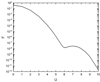 |
Fig. 3. Shape of the complete VDF F with its dependence on the electron velocity U normalized to the thermal electron speed in the upstream region. The shock parameters are X = 1.9, MA = 1.94, and θ = 88.14° with β = 0.29 and γ = 5/3. |
and
 (11)
(11)
respectively.
The conditions under which the reflection takes place can be derived by using Eqs. (2) and (3) to be
 (12)
(12)
The so-called loss-cone angle αlc is defined by αlc = arcsin[(B1/B2)1/2]=arcsin[(1/X)1/2] because of Eq. (8).
After the reflection, the velocity distribution function (VDF) fr of the electrons has the shape of a shifted loss-cone distribution (Leroy & Mangeney 1984; Wu 1984) (see also Eq. (15) in Mann & Klassen 2005) as illustrated in Figs. 3 and 4 in Mann et al. (2018). The VDF fr has both a beam-like and loss-cone-like shape. Hence, there are special regions with both ∂fr/∂V∥ > 0 and ∂fr/∂V⊥ > 0 giving rise to the excitation of plasma waves. Even regions with ∂fr/∂V∥ > 0 lead to the excitation of electrostatic Langmuir waves (Baumjohann & Treumann 1997).
In Sect. 3, the excitation of Langmuir waves is discussed for the case of an initial Maxwellian VDF
 (13)
(13)
in the upstream region. It is normalized to unity. After the reflection via SDA, the reduced VDF
![Mathematical equation: $$ \begin{aligned} F_{\rm acc} = \Theta (V_{\parallel }-V_{\rm s}) \cdot F_{\rm b} \cdot \exp \left(-\frac{[V_{\parallel }-V_{\rm b}]^{2}}{2{ v}_{\rm th,e}^{2}\cos ^{2}\alpha _{\rm lc}}\right) \end{aligned} $$](/articles/aa/full_html/2022/04/aa42201-21/aa42201-21-eq17.gif) (14)
(14)
is found with Vb = Vs(1 + cos2αlc) and
![Mathematical equation: $$ \begin{aligned} F_{\rm b} = \frac{1}{(2\pi { v}_{\rm th,e}^{2})^{1/2}} \cdot e^{-[V_{\rm s}^{2}\sin ^{2}\alpha _{\rm lc} + V_{\rm e}^{2}\tan ^{2}\alpha _{\rm lc}]/2{ v}_{\rm th,e}^{2}} \end{aligned} $$](/articles/aa/full_html/2022/04/aa42201-21/aa42201-21-eq18.gif) (15)
(15)
for the reflected electrons (see Eqs. (17)–(19) in Mann et al. 2018). Here, the Θ(x) is the well-known step function, that is Θ(x) = 1 and Θ(x) = 0 for x ≥ 0 and x < 0, respectively. The reduced VDF is obtained by integrating the usual VDF with respect to the velocity component perpendicular to the magnetic field. We note that Facc represents a distribution function of an electron beam with the velocity Vb and the width 21/2vth,e cos αlc.
3. Excitation of Langmuir waves
The resonant interaction of the beam electrons with the surrounding plasma waves leads to the excitation of Langmuir waves. The resonance condition is given by
 (16)
(16)
where ωL is the frequency of the Langmuir wave and k is the wave number of the Langmuir wave (Baumjohann & Treumann 1997). In addition, Vres is the velocity of the electrons resonantly interacting with the Langmuir waves, and ωL is related to k by the dispersion relation
 (17)
(17)
(Baumjohann & Treumann 1997). Introducing dimensionless quantities according to ν = ωL/ωpe and q = kλDe with the Debye length λDe, the dispersion relation (see Eq. (17)) and the resonance condition (see Eq. (16)) can be written as
 (18)
(18)
and
 (19)
(19)
with Ures = Vres/vth, e leading to
 (20)
(20)
and
 (21)
(21)
respectively. The growth rate γ of Langmuir waves is given by Eq. (4.3) in Treumann & Baumjohann (1997), which can be expressed by
 (22)
(22)
taken at U = Ures = ν/q. Here, F(U) is the reduced VDF, where U denotes the electron velocities normalized to the thermal one. As is well known, wave growth and damping occurs for dF/dU > 0 and dF/dU < 0, respectively.
The full reduced VDF consists of the VDF of the background plasma FM, which is a Maxwellian one (see Eq. (13))
 (23)
(23)
and of the VDF Facc of the accelerated electrons (see Eqs. (15) and (16))
 (24)
(24)
with
 (25)
(25)
where U = V∥/vth, e, Us = Vs/vth, e, and Ub = Vb/vth, e = Us ⋅ (1 + cos2αlc). The complete VDF F is given by F = Facc + FM with Eqs. (23) and (24). For illustration purposes, it is presented in Fig. 3 for a temperature of 1.4 MK and a shock with the parameters X = 1.9, MA = 1.94, and θ = 88.14° as well as β = 0.29 and γ = 5/3. Employing the plasma parameters at the 25 MHz level in the corona as given in Sect. 1, this shock has a velocity of 708 km s−1 and of 21 813 km s−1 in the laboratory and de Hoffmann-Teller frame, respectively. It provides an electron beam with the velocity of 32 145 km s−1 corresponding to a kinetic energy of 3 keV. We note that such a shock is discussed in more detail in Sect. 4. The component of the thermal and accelerated electrons is evidently seen. The VDF shows a local minimum and maximum at U = 6.10 and U = 7.00, respectively. Hence, F has a positive slope in the region 6.10 < U < 7.00, where an instability and, consequently, wave growing occur.
With F = Facc + FM and Eqs. (23) and (24), one gets
![Mathematical equation: $$ \begin{aligned} \frac{\mathrm{d}F}{\mathrm{d}U} =&\frac{1}{(2\pi )^{1/2}}\nonumber \\&\times \left[\frac{(U_{\rm b}-U)}{\cos ^{2} \alpha _{\rm lc}} \cdot F_{\rm b} \cdot e^{-(U-U_{\rm b})^{2}/2\cos ^{2} \alpha _{\rm lc}} - U \cdot e^{-U^{2}/2}\right] \end{aligned} $$](/articles/aa/full_html/2022/04/aa42201-21/aa42201-21-eq29.gif) (26)
(26)
in the region U > Us. Wave growing requires dF/dU > 0 and, hence, U < Ub. The first term on the right-hand side of Eq. (26) has a local maximum at Umax = Ub − cos αls, that is to say wave growing is mostly efficient for electrons with velocities
 (27)
(27)
Equation (27) means that a definite resonance velocity Ures is related to a given shock speed Us. In other words, each individual shock has its own resonance velocity. Inserting U = Ures into Eq. (26) and the thusly obtained expression for dF/dU taken at U = Ures into Eq. (22), one gets for the maximum growth rate
![Mathematical equation: $$ \begin{aligned} \frac{\gamma _{\rm max}}{\omega _{\rm pe}} = \sqrt{\frac{\pi }{8}} \cdot U_{\rm res} \sqrt{U_{\rm res}^{2}-3} \cdot \left[\frac{F_{\rm b,max} \cdot e^{-1/2}}{\cos \alpha _{\rm lc}} - U_{\rm res} \cdot e^{U_{\rm res}^{2}/2}\right] \end{aligned} $$](/articles/aa/full_html/2022/04/aa42201-21/aa42201-21-eq31.gif) (28)
(28)
with
![Mathematical equation: $$ \begin{aligned} F_{\rm b,max} = \exp \left(-\frac{1}{2} \left[\frac{(U_{\rm res} + \cos \alpha _{\rm lc})^{2}}{(1 + \cos ^{2} \alpha _{\rm lc})^{2}} \cdot \sin ^{2} \alpha _{\rm lc} + U_{\rm e}^{2} \cdot \tan ^{2} \alpha _{\rm lc}\right]\right). \end{aligned} $$](/articles/aa/full_html/2022/04/aa42201-21/aa42201-21-eq32.gif) (29)
(29)
Here, Eqs. (20) and (21) have been used. For illustration purposes, the dependence of the growth rate γmax/ωpe on the resonant electron velocity Ures is drawn in Fig. 4. It shows that thermal wave damping occurs until Ures = 5.97. There, wave damping changes into wave growing. Beyond this value, the growth rate rapidly increases up to γmax/ωpe = 1.17 × 10⁻⁶ at Ures = 6.3. Subsequently, it falls down exponentially. Concerning Fig. 4, we note once again that the resonance velocity Ures is related to the shock speed Us according to Eq. (27), in other words, a shock with the speed Us belongs to a fixed resonance velocity Ures.
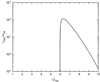 |
Fig. 4. Dependence of the growing rate γmax/ωpe on the velocity Ures of the resonant electrons. We note that γ and β were chosen to be 5/3 and 0.29, respectively. |
Figure 4 shows that the growth rate γmax/ωpe has a clear maximum. In Table 1, the dependence of the maximum max(γmax/ωpe) of the growth rate on the shock strength expressed by the density jump X across the shock is calculated and presented in Fig. 5. Inspecting Table 1, the velocity of electrons resonantly interacting with the electrons for growing Langmuir waves decreases from Ures = 7.3 down to Ures = 6.3 with increasing X in the range X < 1.9 and, subsequently, it increases with increasing X. A shock with X = 1.9 and MA = 1.94 produces, in the most efficient way, energetic electrons which generate Langmuir waves with a maximum growth rate of max(γmax/ωpe) = 1.17 × 10⁻⁶. The electrons resonantly interact with the Langmuir waves which have a velocity Ures = 6.3 in this case.
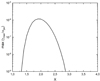 |
Fig. 5. Dependence of the maximum max(γmax/ωpe) of the growing rate on the density jump X across the shock. Again β = 0.29 and γ = 5/3 were chosen. |
4. Discussion
In Sect. 3, it was demonstrated that the electrons accelerated by SDA are able to excite Langmuir waves under plasma conditions at the 25 MHz-level in the corona. These Langmuir waves convert non-linearily into radio waves (Melrose 1985) observed as type II radio bursts. Which growth rate of Langmuir waves is needed for type II radio bursts? Looking to Fig. 1, where a typical example of a solar type II radio burst is presented, the herringbones are the elementary features as mentioned in Sect. 1. They appear for ≈1 s at a fixed frequency. Hence, an enhanced Langmuir wave level should be produced within 0.1 s. The enhancement of the electric field E related to the Langmuir wave by a factor of 10, 100, and 1000 above the thermal one Etherm according to
 (30)
(30)
require a growth rate γmax/ωpe = 1.47 × 10⁻⁷, 2.93 × 10⁻⁷, and 4.40 × 10⁻⁷, respectively. The energy density wL, therm of the thermal level of Langmuir waves is given by
 (31)
(31)
(Krall & Trivelpiece 1973). Adopting the plasma parameters of the 25 MHz level, wL, therm = 7.0 × 10⁻¹³ Ws m−3 is found with λDe = 3 cm and kBT = 120 eV. Hence, the Langmuir waves are associated with electric fields of 0.4 V m−1 on the thermal level. For instance, an enhancement of the electric field of 100 with respect to the thermal one is considered for discussion. Then, γmax/ωpe ≥ 2.93 × 10⁻⁷ is required. This condition is fulfilled for shock parameters in the ranges 1.55 < X < 2.37 and 1.59 < MA < 2.53 (see Table 1 and Fig. 5). Thus, coronal shock waves with a moderate strength are able to accelerate electrons and to generate Langmuir waves. Thus, the solar type II burst emission should be produced by such shocks.
This scenario happens in the most efficient way for coronal shocks with X = 1.9 and MA = 1.94 as revealed by the inspection of Table 1. This special case will be discussed in a little more detail. The plasma parameters usually found in the sources of solar type II bursts (see seventh paragraph in Sect. 1) will be employed for doing that. Because of Eq. (8), the jump in the magnetic field is B2/B1 = X = 1.9, leading to a loss-cone angle αlc = 46.51°. The shock speed vs = MAvA is found to be 710 km s−1 by using MA = 1.94 and an Alfven speed vA = 365 km s−1. In this special case, the Langmuir waves responsible for the radio waves are generated by electrons with a velocity of 29 000 km s−1 because of Ures = 6.3 (see Table 1) and vth, e = 4600 km s−1 as the thermal electron velocity. Because of Ures = Ub − cos αlc = Us(1 + cos2αlc)−cos αlc (see Eq. (27)) Ub = 7.00 is derived and leads to a beam velocity of 32 000 km s−1 corresponding to a kinetic energy of 2.9 keV. Furthermore, the shock speed Us = Ub/(1 + cos2αlc) = 4.75 (or 22 000 km s−1) in the de Hoffmann-Teller frame is obtained by using a thermal electron velocity of vth, e = 4600 km s−1. We note that the shock speed Vs in the de Hoffmann-Teller frame is defined by Vs = vssec θ. Then, θ = 88.14° is found for the angle between the upstream magnetic field and the shock normal, that is to say it is a nearly perpendicular shock geometry. Hence, the Alfven-Mach number  in the de Hoffmann-Teller frame is found to be 60. For the special event on 25 August 2014 (see Fig. 1), a radial velocity vs, r = 556 km s−1 (see sixth paragraph of Sect. 1) was derived for the shock associated with the solar type II radio burst. Since a typical shock velocity vs = 710 km s−1 is expected at the 25 MHz level (see seventh paragraph of Sect. 1) the shock normal takes an angle αr = arccos(vs, r/vs) = 38.45° with respect to the radial direction. Here, there are two different angles. That is the angle θ of the shock normal and the upstream magnetic field and the angle αr between the shock normal and the radial direction. We note that the magnetic field does not necessarily need to be radially directed in the source region of solar type II radio bursts.
The growth rate γmax/ωpe = 1.17 × 10⁻⁶ leads to γmax = 183 s−1 and  = 5.4 ms, that is the energy density of Langmuir waves is rapidly enhanced above the thermal level. According to Eq. (21), the excited Langmuir waves have a frequency ωL = 1.04 ωpe.
The number density of accelerated electrons can be calculated by integrating the reduced distribution function Facc(U) with respect to U, providing
![Mathematical equation: $$ \begin{aligned} \frac{N_{\rm acc}}{N_{1}} =&\exp (-[U_{\rm s}^{2}\sin ^{2}\alpha _{\rm lc} + U_{\rm e}^{2}\tan ^{2}\alpha _{\rm lc}]/2)\nonumber \\&\times \frac{\cos \alpha _{\rm lc}}{2}\left[1 + 2\Phi _{0}(U \cos \alpha _{\rm lc})\right] \end{aligned} $$](/articles/aa/full_html/2022/04/aa42201-21/aa42201-21-eq37.gif) (32)
(32)
with
 (33)
(33)
Employing the above given parameters, one find Nacc/N1 = 5.0 × 10⁻⁸ (Nacc = 0.39 cm−3), that is only a very tiny part of the upstream electrons are finally accelerated up to an energy of a few keV. These electrons carry an energy density  = 1.8 × 10⁻⁹ erg cm−3.
Solar type II radio bursts have typical fluxes of 1000 sfu (see e.g. Nelson & Melrose 1985) at 1 AU (1 AU = 1.496 × 10⁸ km, 1 AU) (1 sfu = 10−22 W m−2 Hz−1 = 10−19 erg cm−2 s−1 Hz−1). The radio flux in the frequency intervall Δf at 1 AU is related to the energy density wradio of the radio waves at the emission site in the corona by
 (34)
(34)
where c is the velocity of light. Then, wradio ≈ 1.5 × 10⁻¹⁶ erg cm−3 is obtained with Δf = 1 MHz. Thus, the energy density of the electron beam is much greater than the energy density of the emitted radio waves, that is to say the electrons accelerated by SDA at a coronal shock have sufficiently enough energy to generate the radio waves which are observed as type II radio bursts.
5. Summary
Solar type II radio bursts are regarded as the radio signature of shock waves travelling through the corona. Such shocks can be generated either by blast waves due to the pressure pulse of a flare and/or driven ahead of CMEs. If these shocks penetrate into interplanetary space, they can be observed as interplanetary type II radio bursts. Coronal shocks are able to accelerate electrons by means of SDA. SDA produces a shifted loss-cone VDF for the energetic electrons. This VDF has both a beam-like and a loss-cone component. The beam-like component is able to excite Langmuir wave, which can be converted into escaping radio waves seen as type II radio emission.
Under coronal circumstances, Langmuir waves are efficiently excited by a shock wave with moderate strength, that is the density jump X across the shock and the Alfven-Mach number are in the ranges 1.55 < X < 2.37 and 1.59 < MA < 2.53, respectively. Thus, solar type II radio bursts are associated with shocks of moderate Alfven-Mach numbers. This result explains why type II radio burst observations provide only moderate Alfven-Mach numbers of the associated shocks (see e.g. Vršnak et al. 2002; Warmuth & Mann 2005; Magdalenic et al. 2020). For plasma conditions at the 25 MHz level in the corona, a shock wave with X = 1.9 and MA = 1.94 produces Langmuir waves in the most efficient way. In this case, the maximum growing rate is γmax = 184 s−1, which rapidly provides an enhanced Langmuir wave level above the thermal one within 5.4 ms. The conversion of Langmuir waves into escaping radio waves has been treated by Schmidt & Cairns (2012a,b) and Schmidt et al. (2014), for instance.
Coronal shock waves are able to produce electrons up to energies of a few keV by SDA. However, only a small fraction of the order of 10−8 are finally accelerated. These electrons carry an energy density of 1.8 × 10⁻⁹ erg cm−3, but that is sufficient enough to generate radio waves with an energy density of 1.5 × 10⁻¹⁶ erg cm−3 at the emission site in the corona in order to provide the observed type II radio fluxes at 1 AU.
For the same event, Magdalenic et al. (2020) obtained a radial velocity of the type II burst source of 800 km s−1 by employing a 3.5-fold Saito (1970) density model, whereas the density model by Mann et al. (1999) is adopted in this paper leading to the difference in the radial type II burst velocities.
References
- Aurass, H. 1996, in Coronal Physics from Radio and Space Observations, ed. G. Trottet (Heidelberg: Springer-Verlag), Lect. Notes Phys., 135 [Google Scholar]
- Aurass, H., & Mann, G. 2004, A&A, 615, 526 [Google Scholar]
- Aurass, H., Vršnak, B., & Mann, G. 2002, A&A, 384, 273 [NASA ADS] [CrossRef] [EDP Sciences] [Google Scholar]
- Ball, L., & Melrose, D. B. 2001, PASA, 18, 361 [NASA ADS] [CrossRef] [Google Scholar]
- Baumjohann, W., & Treumann, R. A. 1997, Basic Space Plasma Physics (London: Imperial College Press), 202 [Google Scholar]
- Cai, Q., Shen, C., Raymond, J. C., et al. 2019, MNRAS, 489, 3183 [Google Scholar]
- Cairns, I. H., & Robinson, R. D. 1987, Sol. Phys., 111, 365 [Google Scholar]
- Cairns, I. H., Knock, S. A., Robinson, P. A., & Kunic, Z. 2003, Space Sci. Rev., 107, 27 [NASA ADS] [CrossRef] [Google Scholar]
- Cane, H. V., Sheeley, N. R., & Howard, R. A. 1987, J. Geophys. Res., 92, 9869 [NASA ADS] [CrossRef] [Google Scholar]
- Dickel, J. 1991, The Radio Spectra of Supernova Remnants (New York: Springer-Verlag) [Google Scholar]
- Dorovskyy, V. V., Melnik, V. N., Konovalenko, A. A., et al. 2015, Sol. Phys., 290, 2031 [NASA ADS] [CrossRef] [Google Scholar]
- Dulk, G. A., & McLean, D. J. 1978, A&A, 66, 315 [NASA ADS] [Google Scholar]
- Forbes, T. G. 1986, ApJ, 305, 553 [NASA ADS] [CrossRef] [Google Scholar]
- Ginzburg, V. L., & Zheleznyakov, V. V. 1958, Sov. Astron., 2, 653 [NASA ADS] [Google Scholar]
- Gopalswamy, N. 2006, J. Air Waste Manage. Assoc., 27, 243 [Google Scholar]
- Gopalswamy, N., Aguilar-Rodriguez, E., Yashiro, S., et al. 2005, J. Geophys. Res., 110, A12S07 [NASA ADS] [CrossRef] [Google Scholar]
- Goodrich, C. C., & Scudder, J. D. 1984, J. Geophys. Res., 89, 6654 [NASA ADS] [CrossRef] [Google Scholar]
- Holman, G. D., & Pesses, M. E. 1983, ApJ, 267, 837 [NASA ADS] [CrossRef] [Google Scholar]
- Hundhausen, A. J., Sawyer, C. B., House, L. L., Illing, R. M. E., & Wagner, W. J. 1984, J. Geophys. Res., 89, 2639 [NASA ADS] [CrossRef] [Google Scholar]
- Klassen, A., Gomez-Herrera, R., Böhm, E., et al. 2008, Ann. Geophys., 26, 901 [Google Scholar]
- Krall, N. A., & Trivelpiece, A. W. 1973, Principles of Plasma Physics (New York: McGraw-Hill) [Google Scholar]
- Krimigis, S. M. 1992, Space Sci. Rev., 59, 167 [NASA ADS] [CrossRef] [Google Scholar]
- Kouloumvakos, A., Rouillard, A., Warmuth, A., et al. 2021, ApJ, 513, 34 [Google Scholar]
- Koutchmy, S. 1994, Adv. Space Res., 14, 29 [CrossRef] [Google Scholar]
- Kunic, Z., Cairns, I. H., & Knock, S. A. 2001, J. Geophys. Res., 107, 101029 [Google Scholar]
- Leroy, M. M., & Mangeney, A. 1984, Ann. Geophys., 2, 449 [NASA ADS] [Google Scholar]
- Magdalenic, J., Marque, C., Zhukov, A. N., Vršnak, B., & Veronig, A. 2012, ApJ, 746, 152 [NASA ADS] [CrossRef] [Google Scholar]
- Magdalenic, J., Marque, C., Fallows, R. A., et al. 2020, ApJ, 897, L15 [NASA ADS] [CrossRef] [Google Scholar]
- Mann, G. 1995, in Coronal Magnetic Energy Release, eds. A. O. Benz, & A. Krüger (Heidelberg: Springer-Verlag), Lect. Notes Phys., 183 [NASA ADS] [CrossRef] [Google Scholar]
- Mann, G. 2006, Solar Eruptions and Energetic Particles (Washington, DC: AGU), 221 [Google Scholar]
- Mann, G., & Klassen, A. 2002, Proc. 10th European Solar Physics Meeting, Prague, Czech Rep., ESA SP-506, 245 [Google Scholar]
- Mann, G., & Klassen, A. 2005, A&A, 441, 319 [NASA ADS] [CrossRef] [EDP Sciences] [Google Scholar]
- Mann, G., Jansen, F., MacDowall, R. J., Kaiser, M. L., & Stone, R. G. 1999, A&A, 348, 614 [NASA ADS] [Google Scholar]
- Mann, G., Warmuth, A., & Aurass, H. 2009, A&A, 394, 669 [NASA ADS] [CrossRef] [EDP Sciences] [Google Scholar]
- Mann, G., Melnik, V. N., Rucker, H. O., Konovalenko, A. A., & Brazhenko, A. I. 2018, A&A, 609, A41 [NASA ADS] [CrossRef] [EDP Sciences] [Google Scholar]
- Melnik, V. N., Konovalenko, A. A., Rucker, H. O., et al. 2004, Sol. Phys., 222, 151 [NASA ADS] [CrossRef] [Google Scholar]
- Melnik, V. N., Rucker, H. O., Konovalenko, A. A., et al. 2008, Solar Physics Research Trends (New York: Nova Science Publishers), 287 [Google Scholar]
- Melrose, D. 1985, Solar Radio Physics (Cambridge: Cambridge University Press), 177 [Google Scholar]
- Nelson, G. S., & Melrose, D. 1985, Solar Radio Physics (Cambridge: Cambridge University Press), 333 [Google Scholar]
- Parker, E. N. 1958, ApJ, 128, 664 [Google Scholar]
- Priest, E. R. 1982, Solar Magnetohydrodynamics (Dordrecht: Kluwer Academic Publishers), 1999 [Google Scholar]
- Rouillard, A. P., Plotnikov, I., Pinto, R. F., et al. 2016, ApJ, 833, 45 [NASA ADS] [CrossRef] [Google Scholar]
- Saito, K. 1970, Ann. Tokyo Astron. Obs., 12, 51 [Google Scholar]
- Schmidt, J. M., & Cairns, I. H. 2012a, J. Geophys. Res., 117, A04106 [NASA ADS] [Google Scholar]
- Schmidt, J. M., & Cairns, I. H. 2012b, J. Geophys. Res., 117, A11104 [NASA ADS] [Google Scholar]
- Schmidt, J. M., Cairns, I. H., & Lobzin, V. V. 2014, J. Geophys. Res., 119, 6042 [NASA ADS] [CrossRef] [Google Scholar]
- Shen, C., Kong, X., Guo, F., Raymond, J. C., & Chen, B. 2018, ApJ, 869, 116 [NASA ADS] [CrossRef] [Google Scholar]
- Shibata, K., Masuda, S., Shimojo, M., et al. 1995, ApJ, 451, L83 [Google Scholar]
- Smerd, S. F., Wild, J. P., & Sheridan, K. V. 1962, Aust. J. Phys., 15, 180 [NASA ADS] [CrossRef] [Google Scholar]
- Stewart, R. T., Howard, R. A., Hansen, F., Gergely, T., & Kundu, M. R. 1974a, Sol. Phys., 36, 219 [NASA ADS] [CrossRef] [Google Scholar]
- Stewart, R. T., McCabe, M., Koomen, M. J., Hansen, F., & Dulk, G. 1974b, Sol. Phys., 26, 203 [NASA ADS] [CrossRef] [Google Scholar]
- Temmer, M., Vršnak, B., Zic, T., & Veronig, A. M. 2009, ApJ, 702, 1343 [NASA ADS] [CrossRef] [Google Scholar]
- Treumann, R. A., & Baumjohann, W. 1997, Advance Space Plasma Physics (London: Imperial College Press), 69 [CrossRef] [Google Scholar]
- Uchida, Y. 1960, PASJ, 12, 376 [NASA ADS] [Google Scholar]
- Uchida, Y., Altschuler, D., & Newkirk, G. 1973, Sol. Phys., 28, 495 [NASA ADS] [CrossRef] [Google Scholar]
- van Haarlem, M. P., Wise, M. W., Gunst, A. W., et al. 2013, A&A, 556, A2 [NASA ADS] [CrossRef] [EDP Sciences] [Google Scholar]
- Vršnak, B., Ruždjak, V., & Aurass, H. 1995, Sol. Phys., 158, 331 [NASA ADS] [Google Scholar]
- Vršnak, B., Aurass, H., Magdalenic, J., & Gopalswamy, N. 2001, A&A, 377, 321 [NASA ADS] [CrossRef] [EDP Sciences] [Google Scholar]
- Vršnak, B., Magdalenic, J., Aurass, H., & Mann, G. 2002, A&A, 396, 673 [NASA ADS] [CrossRef] [EDP Sciences] [Google Scholar]
- Warmuth, A., & Mann, G. 2005, A&A, 435, 1123 [NASA ADS] [CrossRef] [EDP Sciences] [Google Scholar]
- Wild, J. P., & McCready, L. L. 1950, Aust. J. Sci. Res. A Phys. Sci., 3, 387 [Google Scholar]
- Wild, J. P., & Smerd, S. F. 1972, ARA&A, 10, 159 [Google Scholar]
- Wu, C. S. 1984, J. Geophys. Res., 89, 8857 [NASA ADS] [CrossRef] [Google Scholar]
- Zucca, P., Morodan, D. E., Rouillard, A. P., et al. 2018, A&A, 615, A89 [NASA ADS] [CrossRef] [EDP Sciences] [Google Scholar]
- Wu, Y., Rouillard, A. O., Kouloumvakos, A., et al. 2021, ApJ, 909, 163 [NASA ADS] [CrossRef] [Google Scholar]
All Tables
All Figures
|
Fig. 1. Dynamic radio spectrum in the frequency range 10−90 MHz as recorded with the radio telescope LOFAR during the period 15:10−15:30 UT on 25 August 2014 The intensity is colour coded in arbitrary units as seen in the bar on the right-hand side (adapted from Magdalenic et al. 2020). |
| In the text | |
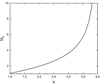 |
Fig. 2. Dependence of MA on X according to Eq. (9) for β = 0.29 and γ = 5/3. |
| In the text | |
|
Fig. 3. Shape of the complete VDF F with its dependence on the electron velocity U normalized to the thermal electron speed in the upstream region. The shock parameters are X = 1.9, MA = 1.94, and θ = 88.14° with β = 0.29 and γ = 5/3. |
| In the text | |
|
Fig. 4. Dependence of the growing rate γmax/ωpe on the velocity Ures of the resonant electrons. We note that γ and β were chosen to be 5/3 and 0.29, respectively. |
| In the text | |
|
Fig. 5. Dependence of the maximum max(γmax/ωpe) of the growing rate on the density jump X across the shock. Again β = 0.29 and γ = 5/3 were chosen. |
| In the text | |
Current usage metrics show cumulative count of Article Views (full-text article views including HTML views, PDF and ePub downloads, according to the available data) and Abstracts Views on Vision4Press platform.
Data correspond to usage on the plateform after 2015. The current usage metrics is available 48-96 hours after online publication and is updated daily on week days.
Initial download of the metrics may take a while.