| Issue |
A&A
Volume 665, September 2022
|
|
|---|---|---|
| Article Number | A98 | |
| Number of page(s) | 7 | |
| Section | The Sun and the Heliosphere | |
| DOI | https://doi.org/10.1051/0004-6361/202243175 | |
| Published online | 15 September 2022 | |
Diagnostics of the dynamics of the Langmuir spectrum based on radio emission during the 12 March 2015 solar radio burst
1
Ioffe Institute, 26 Politekhnicheskaya, 194021 St. Petersburg, Russia
e-mail: igor.koudriavtsev@mail.ioffe.ru
2
Central Astronomical Observatory of RAS, St. Petersburg, Pulkovskoe shosse 65/1 196140, Russia
3
Special Astrophysical Observatory of RAS, Pulkovskoe shosse 65/2, 196140 St. Petersburg, Russia
e-mail: arles@mail.ru
4
Astronomical Institute ASCR, Fričova 298, 251 65 Ondřejov, Czech Republic
e-mail: marian.karlicky@asu.cas.cz
Received:
22
January
2022
Accepted:
21
June
2022
Aims. We investigate the dynamics of spectra of Langmuir waves in the plasma radiation of solar radio bursts.
Methods. We simulated the radio emission that is formed during the merging of Langmuir waves. The observed frequency spectra of radio bursts were fitted by the model spectrum of Langmuir waves.
Results. We determined shapes of the Langmuir wave spectra, consistent with the solar burst observed in the 0.8–2.0 GHz range on 12 March 2015 by the Ondřejov radiospectrograph. We estimated the sizes of the corresponding radio source for different values of the energy density of Langmuir waves. We present the time evolution of the model Langmuir wave spectra at four instants. Finally, we explain a role of the induced scattering of Langmuir waves in the formation of their spectra.
Key words: Sun: flares / Sun: radio radiation / Sun: oscillations
© I. V. Kudryavtsev et al. 2022
 Open Access article, published by EDP Sciences, under the terms of the Creative Commons Attribution License (https://creativecommons.org/licenses/by/4.0), which permits unrestricted use, distribution, and reproduction in any medium, provided the original work is properly cited.
This article is published in open access under the Subscribe-to-Open model. Subscribe to A&A to support open access publication.
1. Introduction
Radio bursts in decimetric and metric frequency ranges are an integral part of solar flares. Their main types are classified as type I, II, III, IV, and V. Their basic characteristics, together with their fine structures, are described, for example, in books by Kundu (1965), Krueger (1979) and McLean & Labrum (1985). These radio bursts are important because they are used for diagnostics of solar flare plasma. Most of these radio bursts are generated by the so-called plasma emission mechanism (Ginzburg & Zhelezniakov 1958). It is a two-step process where, first, owing to some plasma instability (e.g., the bump-on-tail or double-plasma resonance instability), the plasma (Langmuir or upper-hybrid) waves are generated, and then these waves are converted into the electromagnetic waves observed by radio spectrographs. There are two main conversion processes: (a) the scattering of Langmuir waves on plasma particles, thus giving a radio emission close to the electron plasma frequency; and (b) the merging of two Langmuir waves with the radio emission on the double plasma frequency (see also Tsytovich 1977; Melrose 1980; Willes et al. 1996).
In Ginzburg & Zhelezniakov (1958), the authors came to the conclusion that radio bursts can be the result of the generation of radio emission by a coherent plasma mechanism. Thus, for a plasma density of 108 cm−3, the density of fast electrons should be approximately 106 cm−3. In this paper, the coalescence of excited plasma waves (with a fixed direction of the wave vector k) and plasma waves representing thermal fluctuations is considered.
Unlike in Ginzburg & Zhelezniakov (1958), in Zheleznyakov & Zaitsev (1970), the coalescence of excited plasma waves with plasma waves, the distribution of which was formed after the Rayleigh scattering of excited waves, was considered. The intensity of such scattered plasma waves exceeds the level of thermal fluctuations, which increases the efficiency of the transformation of Langmuir waves into transverse electromagnetic waves. In Zheleznyakov & Zaitsev (1970), the authors assumed the density of fast electrons as approximately (1 − 10) cm−3 to explain the intensity of radio emission of type III bursts in the background solar plasma density 108 cm−3.
Furthermore, in Zaitsev & Stepanov (1983) the excitation of Langmuir waves was considered as a result of the loss-cone instability, and a sufficient energy density of Langmuir waves Wl ∼ (10−8 − 10−6)nkbT was estimated to explain the observed radiation from flare kernels with a linear size of the emitting region of 108 cm.
According to Liperovskiǐ & Tsytovich (1969) and Tsytovich (1977), the induced scattering of Langmuir waves on background plasma particles is the key process influencing the resulting spectrum of Langmuir waves. Measuring the fine frequency structure of the spectra of the radio bursts that are formed during the merger of Langmuir waves may allow us to consider the role of the scattering of Langmuir waves in the formation of their spectra, their dynamics, and to diagnose the emitting region.
In this paper we consider the model spectra of plasma waves that allow us to describe the frequency spectra of a radio burst at various time instants during the development of a solar flare on 12 March 2015, assuming that this radio emission is the result of the merger of Langmuir waves. In addition, based on the measured radio emission spectra, we estimate the characteristic size of the radiation region for different values of energy density of Langmuir waves.
The paper is organized as follows. In Sect. 2 we derive the equations and relations necessary for the diagnostics. In Sect. 3 we describe the observational data to which we apply the developed diagnostics. In Sect. 4 we show the results of this diagnosis, and we discuss them in the Sect. 5. In Sect. 6 we summarize the conclusions.
2. Plasma emission formalism
The spectral radiation power of electromagnetic waves with a wave vector k formed by pairwise merging of Langmuir plasmons from a unit volume is determined by the expressions (Tsytovich 1977):
![$$ \begin{aligned} Q_{\boldsymbol{k},\boldsymbol{k_1},\boldsymbol{k_2}}&=\frac{\pi }{8m_{\rm e}} \cdot \frac{\omega }{k^2}\frac{\left( k^2_1-k^2_2\right)^2 \left[\boldsymbol{k_1}\boldsymbol{k_2}\right]^2}{n \, \omega _{\rm pe} \, k_1^2 \, k_2^2} \cdot \delta (\boldsymbol{k}-\boldsymbol{k_1}-\boldsymbol{k_2}) \nonumber \\&\quad \times \delta \left( \sqrt{k^2c^2+\omega ^2_{\rm pe}} -2\omega _{\rm pe} - \frac{3V^2_{\rm Te} \left( k^2_1+k^2_2\right) }{2\omega _{\rm pe} } \right), \end{aligned} $$](/articles/aa/full_html/2022/09/aa43175-22/aa43175-22-eq2.gif)
where k1 and k2 are the wave vectors of two Langmuir plasmons, ω is the frequency of a transverse electromagnetic wave,  is the spectral energy density of Langmuir waves,
  is the electron plasma frequency, e and me are the charge and mass of electrons, ne is the concentration of electrons in the plasma, c is the speed of light,
  is the thermal velocity of the background plasma, kB is the Boltzmann constant, and Te is the temperature of the electron plasma.
The energy density of Langmuir waves is determined by the expression:
Expressions ((1), (2)) define the spectrum of transverse electromagnetic waves formed during the merger of Langmuir waves around the frequency range of approximately 2ωpe, which is discussed in detail in Kudryavtsev & Kaltman (2021). At the same time, even in a homogeneous plasma (i.e., at ne = const.), electromagnetic waves are generated with different frequencies and the width of the frequency spectrum of the generated radio emission can reach ≈20% of a peak frequency or even more. The width of the spectrum of the generated radio radiation is determined by the width of the distribution of Langmuir waves over the wave number k. Thus, in Ratcliffe et al. (2014), it is noted that, if the width of the Langmuir wave spectrum expands to k ∼ 0.2ωpe/VTe, then the width of the radio emission spectrum increases to Δf/f = 0.06, and if the Langmuir wave spectrum expands to k ∼ 0.6ωpe/VTe, then the width of the radio emission spectrum increases to Δf/f = 0.5.
The spectral power of the radio emission generated by this mechanism in a homogeneous plasma of volume V can be written as:

where ϑ and φ are, respectively, the polar and azimuthal angles of the electromagnetic wave vector k. The spectral energy density Qω emitted by a unit volume of plasma is related to the spectral power of radiation by the wave number Qk, for different directions of generation, by the expression:
We can see, for example, a similar formula for the isotropic case in Tsytovich (1977), as well as the work of Kudryavtsev & Kaltman (2021).
In the process of modeling, we set the spectral energy density of Langmuir waves in the form:

where A is a normalization factor. F(k) defines the spectrum of Langmuir waves modulo wave vector and our further goal is to find its correct shape.
The total energy density of Langmuir waves is
where we get the expression for A:
In this paper, we consider the isotropic distribution of Langmuir waves and assume χ(ϑ) = 1.
Using the energy conservation law expressed as ω = ωl(k1)+ωl(k2), where ωl(k) is the Langmuir wave frequency, the minimal and maximal frequency of the radio emission ωmin and ωmax can be estimated as
where kmin and kmax are the minimal and maximal wave vector of Langmuir waves. Therefore, the radio wave frequency ω is in the interval ωmin < ω < ωmax.
The radiation power of transverse electromagnetic waves Q(ϑ, φ) is related to the spectral radiation power Qω(ω, ϑ, φ) by the expression
where

The radiation power of transverse electromagnetic waves Q(ϑ, φ) has the dimension erg cm−3 s−1 sr−1. The spectral power of the radiation Qω(ω, ϑ, φ) has the dimension erg cm−3 sr−1, and Qf(f, ϑ, φ) has the dimension erg cm−3 s−1 sr−1 Hz−1.
Let V be the volume of the radiating region, and S be the area perpendicular to the direction of the Sun at a distance R, where R is 1 AU. The solid angle at which the site S is “visible” from the place of radio emission generation on the Sun is equal to Ω = S/R2.
Then, the spectral power of the radiation through the area S is equal to V ⋅ Qf(f, ϑ, φ)⋅Ω, and the intensity of the radiation (in erg cm−2 s−1 Hz−1):

From Eqs. (1), (6), and (13), it can be seen that Qω(ω, ϑ, φ) and J(f, ϑ, φ) are proportional to (Wl)2. Let the intensity of radio emission with frequency f from the merger of Langmuir waves at a distance of 1 AU be Y sfu. Then the intensity J (in units erg (cm2 s Hz)−1) is equal to:
From Eqs. (1) and (8), it follows that the function Qω(ω, ϑ, φ) is proportional to (Wl)2, and therefore in calculations we use the function qω(ω, ϑ, φ) = Qω(ω, ϑ, φ)/(Wl)2, which is independent of Wl and is determined only by the functions F(k) and χ(ϑ).
Since the shape of the calculated spectrum is determined by the choice of the function F(k), it is sufficient to consider the maximum value Ymax of the radio emission frequency spectrum. We introduce the characteristic size L = V1/3 of the radiation region and obtain an expression relating L to the energy density of Langmuir waves:
where qmax is determined by the type of function F(k), by the plasma parameters, and is calculated using the expression (1), (2), (6), and (8). In next section we model the form of the function F(k) and find the characteristic size L according to the data of radio observations.
3. Observations of the frequency spectra of the 12 March 2015 radio burst
The example of diagnostics is presented for the radio burst shown in Zemanová et al. (2020) that was associated with the complex evolution of a class M1.4 flare (12 Mar. 2015). To analyze the radio emission, we used data from the radio spectrometer in Ondřejov (Jiřička & Karlický 2008) in the range of 0.8–2.0 GHz (Fig. 1).
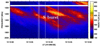 |
Fig. 1. Radio spectrum observed during the 12 March 2015 flare by the Ondřejov radiospectrograph showing slowly positively drifting bursts. The white vertical lines show times of analyzed radio flux vs. frequency plots. |
Several slowly positively drifting bursts recorded from 12:10:20 to 12:10:50 UT with a maximum of about 12:10:40 UT were interpreted in Zemanová et al. (2020) by proton beams propagating into a large filament. Among these slowly positively drifting bursts, the S burst (indicated in Fig. 1) is the most interesting because its S-like form indicates that the beam was propagating through a helical structure of the filament. In this structure the beam was propagating in an almost horizontal direction in the solar atmosphere, or in other words, in a big angle to the density gradient in the gravitationally stratified solar atmosphere. Analyzing times and locations of EUV brightenings at times of the S burst, and modeling of the beam propagation in the helical structure with the filament, Zemanová et al. (2020) estimated the beam velocity to be about 30 000 km s−1. Assuming now that the temperature at the helical structure is 1 MK, then the ratio of the beam velocity and the electron thermal velocity is about 7.7, which is sufficient for Langmuir wave generation (Ginzburg & Zhelezniakov 1958; Benz 1993). At the time of 12:10:36 UT, the S burst begins to appear with a maximum of about 1.1 GHz. At 12:10:43 UT, its peak in the radio flux vs. frequency plot has a maximum at 1.6 GHz.
The development of flare processes affected a vast area of the solar atmosphere (Fig. 2). Observational manifestations in different spectral bands and their possible connection with physical flare processes of magnetic reconnection and particle acceleration were thoroughly analyzed in Zemanová et al. (2020). We note that simultaneously with positively drifting bursts, a plasma jet was observed in the images in the extreme ultraviolet wavelengths of AIA/SDO (Fig. 3). We searched a sequence of images closest to the moment of the start of the S burst, using all available AIA lines to clarify the moment of the appearance of the jet. We found that the jet started at 12:10:24 UT and appeared during a group of slowly positively drifting bursts.
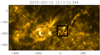 |
Fig. 2. AIA, 171A: The development of flare processes affected a vast area of the solar atmosphere. The area of development of jet is indicated by a black square (see Fig. 3). Data courtesy of the AIA (NASA/SDO) science team. |
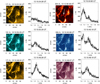 |
Fig. 3. Simultaneously with radio bursts, a plasma jet was observed in the images in the extreme ultraviolet wavelengths of AIA/SDO (data courtesy of the AIA (NASA/SDO) science team). Areas of AIA/SDO images correspond to the area in the black square in Fig. 2. The white arrow points to the jet. |
It is interesting to investigate the features of the dynamics of the frequency profile of the S burst. Despite the rapid small changes in the radio emission profile, most likely occurring faster than the available time resolution of 0.1 s, it is possible to identify a smooth trend of profile changes with time. Over time, the left low-frequency edge of the profile (relative to the maximum frequency) becomes flatter, and the right high-frequency edge becomes sharper, so S burst has a gentle rise and a sharper decline, being in the final stage of its development (Figs. 3 and 4). In next section we demonstrate examples of the possible frequency spectra of the Langmuir wave, which we found to be in accordance with the measured radio emission spectra for four time instants indicated by the white vertical lines on the dynamic spectrum in Fig. 1.
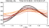 |
Fig. 4. Smoothed profiles of the burst combined by the frequency of the maximum (indicated by the vertical dotted line) between 12:10:36.8 and 12:10:40.7 UT. Every third profile is shown, and the first in time (the darkest) and the last (the lightest) are highlighted with thicker lines. The frequency scale corresponds to the first (initial) profile. |
4. Results: Simulation of S burst for different time instants
In this section we present selected spectra of Langmuir waves that simulate the frequency spectra of the S burst during a pairwise merger of Langmuir plasmons for four time instants. We do not solve the integral equation, Eq. (1), but we simply fit the Langmuir spectra. The coincidence of the shape of the calculated spectrum with the observed one is ensured by the choice of the function F(k).
We consider radio emission as the sum of background radiation and radiation from the merger of Langmuir waves. The value of the coronal temperature taken was 106 K.
The function F(k) of the distribution of Langmuir waves over wave numbers is characterized by several basic parameters: k0, kmin, and kmax, as well as parameters that determine the slopes of the function. The parameter k0 characterizes the region of wave numbers in which the bulk of Langmuir waves is generated. The parameter kmin determines a certain minimum value of the wave numbers, but since the contribution of waves with minimal wave numbers to the resulting radiation is small, this parameter is difficult to accurately estimate, and thus we present the results for its three possible values. The parameter kmax characterizes the breakage of the spectrum from the side of the maximum wave numbers. The found forms of the function F(k) and the values of these and other parameters are given below.
Figure 5 shows the measured and model spectra of the radio burst, as well as the corresponding model spectrum of Langmuir waves for the four time instants. Our estimates of the size of the solar plasma regions in which radio bursts are generated are given in Table 1. Because the emission region size (L) as well as the energy density of Langmuir waves are not known, the size of the emission region is estimated assuming different values of the energy density of Langmuir waves. We also use reconstruction with kmin = wpe/(15VTe), according to Eq. (15). To do this, using Formulas (1)–(6), we calculated the values of the function q(ω), which determine the radio emission spectra for the considered time instants.
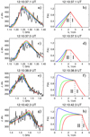 |
Fig. 5. Spectra of radio burst and spectra of Langmuir waves. Left column: measured and model spectra of the radio burst. Right column: corresponding model spectra of Langmuir waves. The calculation results are given for kmin = ωpe/(10VTe), kmin = ωpe/(15VTe), and kmin = ωpe/(60VTe) (red, green, and blue curves, respectively). |
Estimated parameters for selected time instants.
Curves with other kmin in Fig. 5 are constructed for the same volume of the emission region and for the same energy density of Langmuir waves. As can be seen from these figures, an increase in the value of the kmin of the Langmuir spectrum leads not only to a narrowing of the spectrum width of the generated radio emission, but also to a certain increase in the maximum of the radio burst. A decrease in kmin leads to an increase in this width and a decrease in the maximum of the burst.
4.1. Time instant 12:10:37.1 UT
The measured radio spectrum can be modeled with the following function for Langmuir spectra (Figs. 5a and 5b):
The parameters are: δ1 = 1, δ2 = 0.5, and kmax = wpe/(2.3VTe). The function F(k) has a maximum at k0 = wpe/(4.0VTe). The maximum intensity of radiation increases with a decrease in the width of the spectrum of Langmuir waves.
4.2. Time instant 12:10:37.5 UT
The measured radio spectrum can be modeled with the same function, Function (16), for Langmuir spectra, but with a “cut-off” top: if the value of F(k) is greater than Fmax = 0.75, then F(k) = Fmax (Figs. 5c and 5d). The parameters of the function F(k) are: δ1 = 1.5, δ2 = 0.6, kmax = wpe/(2.5VTe), and k0 = wpe/(4.8VTe).
4.3. Time instant 12:10:38.9 UT
We modified the function F(k) in this way:
Parameters of the function F(k) are: γ = 1, δ1 = 0.7, δ2 = 0.5, kmax = wpe/(2.2VTe), and k0 = wpe/(3.3VTe). Figures 5e and 5f show observed and model radio spectra and modeled Langmuir spectrum for this time instant.
4.4. Time instant 12:10:42.3 UT
The measured radio spectrum can be modeled with the same function, Function (17), for Langmuir spectra as previous time instant, but with parameters: γ = 1, δ1 = 0.7, δ2 = 4.0, kmax = wpe/(2.2VTe), and k0 = wpe/(2.7VTe). Figures 5g and 5h show observed and model radio spectra and modeled Langmuir spectrum for this time instant.
4.5. Fitting the spectra for time instant 12:10:42.3 UT
Using the example of the last, most difficult profile, we show in more detail how we adjusted the spectrum of Langmuir waves. Figure 6 illustrates the procedure for selecting the spectrum of Langmuir waves that allows us to simulate the measured radio emission spectrum for the time instant 12:10:42.3 UT.
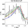 |
Fig. 6. Fitting of parameters for the spectrum at 12:10:42.3 UT. |
First, we set function F(k) in form of Function (17), with γ = 0 for left part of spectrum, and the other parameters were the same as in Sect. 4.4. The corresponding simulated radio emission profile (blue line in Fig. 6) shows that in this form, the function F(k) does not allow us to obtain the spectrum of the radio burst at time 12:10:42.3 UT: the measured spectrum of the burst in the band from 1.4 GHz to 1.6 GHz has an almost linear growth, while the simulated (blue) spectrum of the burst grows stronger with increasing frequency.
The simulated spectrum with γ = 1 (green line) is a much better fit of the observed one. Figure 6 also shows how the parameter k0 affects the calculated radio spectrum. At k0 = ωpe/(2.6VTe) (red line), the maximum of the calculated spectrum of the radio burst is shifted toward higher values of the frequency relative to the case with k0 = ωpe/(2.7VTe)(red and blue lines).
5. Discussion
5.1. Jet and Langmuir turbulence
In the paper by Chen et al. (2018), it is concluded that the particles are accelerated in the area behind the jet spiral, coinciding with the presumed location of magnetic reconnection. In an interpretation of the jet accompanying burst investigated in present paper (Fig. 3), the most probable reason for its appearance is that during the acceleration process of the beam, the plasma close to the acceleration region is heated and also particles slower than beam velocities are accelerated, thus increasing the plasma density in the direction of an accelerated particle motion. We also propose that the jet may indicate a region of enhanced Langmuir turbulence.
5.2. The I and II regions on diagnosed Langmuir spectra
Figure 5 (right column) highlights regions I and II. Langmuir waves are probably generated in the region close to boundary between regions I and II. Region I may correspond to a decrease in the spectral energy density of Langmuir waves as a result of the effective absorption of Langmuir waves with phase velocities less than 3VTe by thermal electrons (the so-called Landau damping). Region II can be interpreted as the region “pumping” the energy of Langmuir waves from waves with large wave numbers to waves with small kl during the induced scattering of these waves on thermal plasma particles. It can be assumed that the generation of these waves occurs in the region of wave numbers  , and the induced scattering of Langmuir waves can lead to the appearance of waves with wave numbers
  (Liperovskiǐ & Tsytovich 1969).
A characteristic feature of the measured spectrum of the radio burst at time instant 12:10:37.5 (Figs. 5c and 5d) is the flat top of the spectrum. This is associated with the horizontal section of the spectrum of Langmuir waves.
Langmuir waves, which spectra are shown in Fig. 5, have phase velocities less than the speed of light c. At the same time, even if in the first two presented time instants the “pumping” of the energy of Langmuir waves from waves with large wave numbers k to waves with small k due to induced scattering by thermal particles is present, this “pumping” does not manifest itself as clearly as in the third and fourth time instants. It should be noted that Langmuir waves with phase velocities greater than  , which may appear as a result of “pumping”, cannot merge into an electromagnetic wave, since the law of conservation of momentum cannot be fulfilled for them (Zheleznyakov 1996).
The widths of region II at time instants 12:10:38.9 UT and 12:10:42.3 UT (Figs. 5f and 5h) indicate that there is a decrease in the number of fast particles in the plasma that generate Langmuir waves and prevent the expansion of the wave spectrum into the region of small k (Liperovskiǐ & Tsytovich 1969). The difference in the calculated frequency spectra of the radio burst in Fig. 5h is very small: at frequencies of 1.4–1.5 GHz, the radiation intensity in the case of  is slightly higher than at
  . With a decrease in
  , the radio emission spectrum flattens. It is impossible to make an unambiguous choice between the options presented in Fig. 5h only on the basis of comparison with the measured spectrum of radio emission. However, the very existence of a significant flat part in region II indicates the existence of induced scattering of Langmuir waves by thermal particles in the solar plasma, where radio emission is generated at 12:10:42.3 UT.
5.3. Induced scattering of Langmuir waves
Having studied the instantaneous profiles of radio spectra for different time instants, we found the effect of flattening the low-frequency edge over time. This is consistent with the effect of a gradual transfer of the energy of Langmuir waves to the region of small wave numbers due to the induced scattering of these waves on thermal ions and plasma electrons (Liperovskiǐ & Tsytovich 1969).
Among nonlinear processes involving Langmuir waves, induced scattering of Langmuir plasmons on electrons (l + e → l′+e′) and plasma ions (l + i → l′+i′), as well as scattering of one Langmuir plasmon on another (l1 + l2 → l3 + l4), is of particular importance for the formation of the spectrum of these waves (Tsytovich 1977). The first two processes lead to the “pumping” of energy from waves with large wave numbers to waves with small k. However, for waves with small wave numbers, the third process (l1 + l2 → l3 + l4) becomes important, which prevents the concentration of Langmuir plasmons in the region k ≈ 0. In this case, a spectrum of Langmuir waves can be formed with a sharp increase and a maximum at a small wave number.
It is well known that induced scattering of Langmuir waves on plasma particles leads to the transformation of the spectrum of these waves: the energy passes from waves with large values of the wave number k to waves with smaller values of k (Liperovskiǐ & Tsytovich 1969). At the same time, it is possible to form a spectrum of Langmuir waves with a maximum at a wavenumber much smaller than the wavenumber kg of generated waves. However, there are processes in the plasma that prevent the formation of such a spectrum of Langmuir waves (Liperovskiǐ & Tsytovich 1969). The first of these processes are the Coulomb collisions of thermal electrons in plasma, which lead to the absorption of waves. Another factor preventing the transformation of the spectrum of Langmuir waves in the region of small wave numbers is the presence of fast (nonthermal) particles in the plasma. As our simulations have shown, the flattening of the radiation spectrum is associated with the broadening of the spectrum of Langmuir waves, and this broadening may be the result of induced scattering of Langmuir waves on plasma particles.
It follows from the above that, based on the measured spectra of radio bursts generated around the frequency range of approximately 2ωpe, it is possible to study the dynamics of the spectra of Langmuir waves in astrophysical plasma and the role of induced scattering of Langmuir waves. Thus, all this allows us to improve the diagnostics of the emitting area.
5.4. A direct and inverse problem
It should be noted that we are not solving a direct problem, but instead we consider the inverse problem. Nevertheless, we compare the wavenumbers obtained by the direct and inverse approach. Taking the maximum flux frequency of the S burst at three times (12:10:37.1, 12:10:38.9, and 12:10:42.3 UT) as about 1250, 1370, and 1600 MHz, we can roughly estimate the wavenumbers obtained from the direct approach as k = ωl/vb ≈ ωpe/vb, for Langmuir waves propagating along the direction of motion of fast particles with a velocity vb, where ωl is the frequency of the Langmuir wave. As f ≈ 2ωpe/(2π) = ωpe/π, then ωpe ≈ πf and k ≈ πf/vb. Using the velocity of fast particles of 30 000 km s−1 estimated in the work of Zemanová et al. (2020), we get k approximately equal to 1.31 cm−1, 1.43 cm−1, and 1.68 cm−1 for f equal to 1250, 1370, and 1600 MHz. The increase in k corresponds to the increase in k in Fig. 5. In our inverse approach, we found that the wavenumbers are higher. The difference in determination of the wavenumbers in the direct and inverse approaches can be explained as follows: we assume that the burst bandwidth is 200 MHz (e.g., between 1300 and 1500 MHz). In our inverse approach, we used the model that is homogeneous in selected times and its density corresponds to the minimum frequency of the burst-frequency profile (1300 MHz in our example), in other words, to the minimum density and plasma frequency. Then, considering the dispersion relation for Langmuir waves, for a description of the full burst bandwidth up to 1500 MHz, the wavenumbers with higher values are necessary comparing to the case with the inhomogeneous densities in the burst source (real case), because in the inhomogeneous source, densities are mostly above the minimum density. Thus, plasma frequencies are above the minimum plasma frequency. Therefore, in the real inhomogeneous model for generation of the maximum burst frequency (1500 MHz), the k-values need not be as high as in the model with the homogenous and minimal source density.
In addition, as noted above, this estimate for k is given only for Langmuir waves that propagate strictly along the direction of motion of fast particles. However, the one-dimensional approximation can be considered only in the case of a strong magnetic field (for example, Tsytovich 1977), that is, when ωBe ≫ ωpe. If this condition is not satisfied, then Langmuir waves are also excited at different angles ϑ to the velocity of fast particles vb, and the resonance condition has the form kvb cos ϑ = ωl or k = ωl/(vb cos ϑ). Therefore, at 0 < ϑ < 90°, the value k will be greater than the above values of k (1.31 cm−1, 1.43 cm−1, and 1.68 cm−1) obtained for ϑ = 0°. We also note that an increase in the plasma temperature decreases the wavenumber values of Langmuir waves, presented in Fig. 5, as kmax ∼ 1/VTe.
6. Conclusions
We present an example of diagnostics for a radio burst associated with the complex evolution of a class M1.4 flare (12 March 2015), which led to the appearance of a plasma jet and simultaneous generations of radio bursts. To analyze the radio emission, we used data from a radio spectrometer in Ondrejov (Czech Republic) in the range of 0.8–2 GHz. We got the following results.
-
Assuming that the observed radio emission is the result of the coalescence of plasma waves, we find such forms of the frequency spectra of Langmuir waves at which the calculated radio emission corresponds to the measured radio spectra.
-
Having studied the instantaneous profiles of radio spectra for individual radio burst structures, we found the effect of the flattening of the low-frequency edge over time.
-
This flattening of the low-frequency edge is consistent with the effect of gradual transfer of the energy of Langmuir waves to the region of small wave numbers due to the induced scattering of these waves on thermal ions and plasma electrons.
-
Induced scattering can cause a large width of the Langmuir spectrum, while the beam width in terms of velocities can be narrow.
The main conclusion we come to is that measuring the fine frequency structure of radio spectra that are formed by merging Langmuir waves can allow us to diagnose the approximate shape of the spectra of Langmuir waves at different time instants. This also allows us to consider the role of the induced scattering of Langmuir waves in the formation of their spectra and their dynamics.
Acknowledgments
I. Kudryavtsev acknowledges support from the Grant 18-29-21016 of the RFBR. T. Kaltman acknowledges support from under the Ministry of Science and Higher Education of the Russian Federation grant 075-15-2022-262 (13.MNPMU.21.0003). M. Karlický acknowledges support from the project RVO-67985815 and GA ČR grants 20-09922J, 20-07908S, 21-16508J and 22-34841S.
References
- Benz, A. O. 1993, Plasma Astrophysics: Kinetic Processes in Solar and Stellar Coronae (Dordrecht: Kluwer Academic Publishers), 184, 175 [NASA ADS] [Google Scholar]
- Chen, B., Yu, S., Battaglia, M., et al. 2018, ApJ, 866, 62 [Google Scholar]
- Ginzburg, V. L., & Zhelezniakov, V. V. 1958, Sov. Astron., 2, 653 [Google Scholar]
- Jiřička, K., & Karlický, M. 2008, Sol. Phys., 253, 95 [CrossRef] [Google Scholar]
- Krueger, A. 1979, Introduction to Solar Radio Astronomy and Radio Physics (Dordrecht: D. Reidel Publ. Comp) [CrossRef] [Google Scholar]
- Kudryavtsev, I. V., & Kaltman, T. I. 2021, MNRAS, 503, 5740 [NASA ADS] [CrossRef] [Google Scholar]
- Kundu, M. R. 1965, Solar Radio Astronomy (New York: Interscience Publication) [Google Scholar]
- Liperovskiǐ, V. A., & Tsytovich, V. N. 1969, Sov. J. Exp. Theoret. Phys., 30, 682 [Google Scholar]
- McLean, D. J., & Labrum, N. R. 1985, Solar Radiophysics: Studies of Emission from the Sun at Metre Wavelengths (Cambridge: Cambridge University Press) [Google Scholar]
- Melrose, D. B. 1980, Plasma Astrophysics: Nonthermal Processes in Diffuse Magnetized Plasmas. Volume 2 - Astrophysical Applications, 212 [Google Scholar]
- Ratcliffe, H., Kontar, E. P., & Reid, H. A. S. 2014, A&A, 572, A111 [NASA ADS] [CrossRef] [EDP Sciences] [Google Scholar]
- Tsytovich, V. N. 1977, Theory of Turbulent Plasma, New York, NY (USA): Consultants Bureau [CrossRef] [Google Scholar]
- Willes, A. J., Robinson, P. A., & Melrose, D. B. 1996, Phys. Plasmas, 3, 149 [NASA ADS] [CrossRef] [Google Scholar]
- Zaitsev, V. V., & Stepanov, A. V. 1983, Sol. Phys., 88, 297 [Google Scholar]
- Zemanová, A., Karlický, M., Kašparová, J., & Dudík, J. 2020, ApJ, 905, 111 [CrossRef] [Google Scholar]
- Zheleznyakov, V. V. 1996, Radiation in Astrophysical Plasmas, Astrophysics & Space Science Library, 204 [CrossRef] [Google Scholar]
- Zheleznyakov, V. V., & Zaitsev, V. V. 1970, AZh, 47, 308 [NASA ADS] [Google Scholar]
All Tables
All Figures
|
Fig. 1. Radio spectrum observed during the 12 March 2015 flare by the Ondřejov radiospectrograph showing slowly positively drifting bursts. The white vertical lines show times of analyzed radio flux vs. frequency plots. |
| In the text | |
|
Fig. 2. AIA, 171A: The development of flare processes affected a vast area of the solar atmosphere. The area of development of jet is indicated by a black square (see Fig. 3). Data courtesy of the AIA (NASA/SDO) science team. |
| In the text | |
|
Fig. 3. Simultaneously with radio bursts, a plasma jet was observed in the images in the extreme ultraviolet wavelengths of AIA/SDO (data courtesy of the AIA (NASA/SDO) science team). Areas of AIA/SDO images correspond to the area in the black square in Fig. 2. The white arrow points to the jet. |
| In the text | |
|
Fig. 4. Smoothed profiles of the burst combined by the frequency of the maximum (indicated by the vertical dotted line) between 12:10:36.8 and 12:10:40.7 UT. Every third profile is shown, and the first in time (the darkest) and the last (the lightest) are highlighted with thicker lines. The frequency scale corresponds to the first (initial) profile. |
| In the text | |
|
Fig. 5. Spectra of radio burst and spectra of Langmuir waves. Left column: measured and model spectra of the radio burst. Right column: corresponding model spectra of Langmuir waves. The calculation results are given for kmin = ωpe/(10VTe), kmin = ωpe/(15VTe), and kmin = ωpe/(60VTe) (red, green, and blue curves, respectively). |
| In the text | |
|
Fig. 6. Fitting of parameters for the spectrum at 12:10:42.3 UT. |
| In the text | |
Current usage metrics show cumulative count of Article Views (full-text article views including HTML views, PDF and ePub downloads, according to the available data) and Abstracts Views on Vision4Press platform.
Data correspond to usage on the plateform after 2015. The current usage metrics is available 48-96 hours after online publication and is updated daily on week days.
Initial download of the metrics may take a while.