| Issue |
A&A
Volume 685, May 2024
|
|
|---|---|---|
| Article Number | A87 | |
| Number of page(s) | 19 | |
| Section | Astrophysical processes | |
| DOI | https://doi.org/10.1051/0004-6361/202348670 | |
| Published online | 08 May 2024 | |
Narrow spectra of repeating fast radio bursts: A magnetospheric origin
1
School of Astronomy and Space Science, University of Chinese Academy of Sciences, Beijing 100049, PR China
2
State Key Laboratory of Nuclear Physics and Technology, School of Physics, Peking University, Beijing 100871, PR China
3
Department of Astronomy, School of Physics, Peking University, Beijing 100871, PR China
e-mail: This email address is being protected from spambots. You need JavaScript enabled to view it.
4
South-Western Institute for Astronomy Research, Yunnan University, Kunming, Yunnan 650504, PR China
5
Purple Mountain Observatory, Chinese Academy of Sciences, Nanjing 210023, PR China
6
Kavli Institute for Astronomy and Astrophysics, Peking University, Beijing 100871, PR China
7
New Cornerstone Science Laboratory, National Astronomical Observatories, Chinese Academy of Sciences, Beijing 100101, PR China
8
Institute for Frontiers in Astronomy and Astrophysics, Beijing Normal University, Beijing 102206, PR China
Received:
20
November
2023
Accepted:
21
February
2024
Abstract
Fast radio bursts (FRBs) can present a variety of polarization properties and some of them are characterized by narrow spectra. In this work, we study spectral properties from the perspective of intrinsic radiation mechanisms and absorption through the waves propagating in the magnetosphere. The intrinsic radiation mechanisms are considered by invoking quasi-periodic bunch distribution and perturbations on charged bunches moving on curved trajectories. The narrowband emission is likely to reflect some quasi-periodic structure on the bulk of bunches, which may be due to quasi-periodically sparking in a “gap” or quasi-monochromatic Langmuir waves. A sharp spike would appear in the spectrum if the perturbations were to induce a monochromatic oscillation of bunches; however, it is difficult to create a narrow spectrum because the Lorentz factor has large fluctuations, so the spike disappears. Both the bunching mechanism and perturbations scenarios share the same polarization properties, with a uniformly distributed bulk of bunches. We investigated the absorption effects, including Landau damping and curvature self-absorption in the magnetosphere, which are significant at low frequencies. Subluminous O-mode photons cannot escape from the magnetosphere due to the Landau damping, leading to a height-dependent lower frequency cut-off. The spectra can be narrow when the frequency cut-off is close to the characteristic frequency of curvature radiation, however, such conditions cannot always be met. The spectral index is 5/3 at low-frequency bands due to the curvature self-absorption is not as steep as what is seen in observations. The intrinsic radiation mechanisms are more likely to generate the observed narrow spectra of FRBs, rather than the absorption effects.
Key words: polarization / radiation mechanisms: non-thermal / stars: magnetars / stars: neutron
© The Authors 2024
 Open Access article, published by EDP Sciences, under the terms of the Creative Commons Attribution License (https://creativecommons.org/licenses/by/4.0), which permits unrestricted use, distribution, and reproduction in any medium, provided the original work is properly cited.
This article is published in open access under the Subscribe to Open model. This email address is being protected from spambots. You need JavaScript enabled to view it. to support open access publication.
1. Introduction
Fast radio bursts (FRBs) are millisecond-duration and energetic radio pulses (see Cordes & Chatterjee 2019; Petroff et al. 2019, for reviews). They are similar in some respects to single pulses from radio pulsars, however, the bright temperature of FRBs is many orders of magnitude higher than that of normal pulses from Galactic pulsars. The physical origin(s) of FRB are still unknown and the only certainty is that their radiation mechanisms must be coherent.
Magnetars have been invoked as the most likely candidate to interpret the emission of FRBs, especially repeating ones. The models can be generally divided into two categories by considering the distance of the emission region from the magnetar (Zhang 2020): emission within the magnetosphere (pulsar-like model, e.g., Katz 2014; Kumar et al. 2017; Yang & Zhang 2018; Wadiasingh & Timokhin 2019; Lu et al. 2020; Cooper & Wijers 2021; Wang et al. 2022a; Zhang 2022; Liu et al. 2023a; Qu & Zhang 2023) and emission from relativistic shocks region far outside the magnetosphere (GRB-like model, e.g., Metzger et al. 2019; Beloborodov 2020; Margalit et al. 2020; Chen et al. 2022; Khangulyan et al. 2022). A magnetar origin for at least some FRBs was established after the detection of FRB 20200428D1, an FRB-like burst from SGR J1935+2154, which is a Galactic magnetar (Bochenek et al. 2020; CHIME/FRB Collaboration 2020a). Nevertheless, the localization of FRB 20200120E to an old globular cluster in M 81 (Bhardwaj et al. 2021; Majid et al. 2021; Kirsten et al. 2022) poses a challenge to the assumption of a young magnetar born via a massive stellar collapse. This would mean that the magnetar formed in accretion-induced collapse or a system associated with a compact binary merger (Kremer et al. 2021; Lu et al. 2022).
The spectral-time characteristics of FRBs are significant tools that are useful for gaining a deeper understanding of emission mechanisms. The burst morphologies of FRBs are varied. Some FRBs have a narrow bandwidth, for instance, with the sub-bursts of FRB 20220912A showing that the relative spectral bandwidth of the radio bursts was distributed near at Δν/ν ≃ 0.2 (Zhang et al. 2023). Similar phenomena of narrowband can appear at FRB 20121102A, in which spectra are modeled by simple power laws with indices ranging from −10 to +14 (Spitler et al. 2016). Simple narrowband and other three features (simple broadband, temporally complex, and downward drifting) are summarized as four observed archetypes of burst morphology among the first CHIME/FRB catalog (Pleunis et al. 2021). The narrow spectra may result from small deflection angle radiation or coherent processes. Alternatively, they could be modulated by scintillation and plasma lensing in the FRB source environment (Yang 2023).
Downward drift in the central frequency of consecutive sub-bursts with later-arriving time, has been discovered in at least some FRBs (CHIME/FRB Collaboration 2019a; Hessels et al. 2019; Fonseca et al. 2020). In addition, a variety of drifting patterns including upward drifting, complex structure, and no drifting subpulse, was found in a sample of more than 600 bursts detected from the repeater source FRB 20201124A (Zhou et al. 2022). Such a downward drifting structure was unprecedentedly seen in pulsar PSR B0950+08 (Bilous et al. 2022), suggesting that FRBs originate from the magnetosphere of a pulsar. Downward drifting patterns can be aptly understood by invoking magnetospheric curvature radiation (Wang et al. 2019), however, it is unclear why the spectral bandwidth can be extremely narrow, namely, Δν/ν ≃ 0.1.
Polarization properties carry significant information about radiation mechanisms to shed light on the possible origin of FRBs. High levels of linear polarization are dominant for most sources and most bursts for individual repeating sources (e.g., Michilli et al. 2018; Day et al. 2020; Luo et al. 2020; Sherman et al. 2023), while some bursts have significant circular polarization fractions, which can be even up to 90% (e.g., Masui et al. 2015; Xu et al. 2022; Jiang et al. 2022; Kumar et al. 2022). The properties are reminiscent of pulsars, which show a wide variety of polarization fractions between sources. The emission is highly linearly polarized when the line of sight (LOS) is confined into a beam angle, whereas highly circular polarization is present when the LOS is outside, when considering bunched charges moving at ultra-relativistic speed in the magnetosphere (Wang et al. 2022b; Liu et al. 2023b).
In this work, we attempt to understand the origin(s) of the observed narrow spectra of FRBs from the perspective of intrinsic radiation mechanisms and absorption effects in the magnetosphere. The paper is organized as follows. The intrinsic radiation mechanisms by charged bunches in the magnetosphere are discussed in Sect. 2. We investigate two scenarios of the spectrum, including the bunch mechanism (Sect. 2.1) and perturbations on the bunch moving at curved trajectories (Sect. 2.2). The polarization properties of the intrinsic radiation mechanisms are summarized in Sect. 2.3. In Sect. 3, we discuss several possible mechanisms as triggers that may generate emitting charged bunches (Sect. 3.1), as well as oscillations and Alfvén waves. Some absorption effects during the wave propagating in the magnetosphere are investigated in Sect. 4. We discuss the bunch’s evolution in the magnetosphere in Sect. 5. The results are discussed and summarized in Sects. 6 and 7. The convention Qx = Q/10x in cgs units and spherical coordinates (r, θ, φ) relating to the magnetic axis are used throughout the paper.
2. Intrinsic radiation mechanism
A sudden trigger may occur on the stellar surface and last at least a few milliseconds to create free charges. Such a trigger event is a sudden and violent process in contrast to a consecutive “sparking” process in the polar cap region of a pulsar (Ruderman & Sutherland 1975). The charges can form bunches and the total emission of charges is coherently enhanced significantly if the bunch size is smaller than the half wavelength. We note that electrons as the emitting charges are the point of interest in the following discussion, leading to negatively net-charged bunches. We attempt to study how to trigger the emitting charges and how to form bunches in Sect. 3.
Within the magnetosphere, the charged particles are suddenly accelerated to ultra-relativistic velocities and stream outward along the magnetic field lines. The charges hardly move across the magnetic field lines because the cyclotron cooling is very fast in a strong magnetic field and charges stay in the lowest Landau level so that charges’ trajectories essentially track with the field lines.
Curvature radiation can be produced via the perpendicular acceleration for a charge moving at a curved trajectory. It is a natural consequence that charges moving at curved trajectories, which has been widely discussed in pulsars (Ruderman & Sutherland 1975; Cheng & Ruderman 1977; Melikidze et al. 2000; Gil et al. 2004; Gangadhara et al. 2021) and FRBs (Kumar et al. 2017; Katz 2018; Lu & Kumar 2018; Ghisellini & Locatelli 2018; Yang & Zhang 2018; Wang et al. 2022a; Cui et al. 2023). However, the noticeable difference is that there should be an electric field parallel (E∥) to the local magnetic field B in the FRB emission region because the enormous emission power of FRB lets the bunches cooling extremely fast. The E∥ sustains the energy of bunches so that they can radiate for a long enough time to power FRBs. The equation for motion in the FRB emission region in the lab frame can be written as:
 (1)
(1)
where Ne is the number of net charges in one bunch that are radiating coherently, c is the speed of light, e is the elementary charge, me is the positron mass, γ is the Lorentz factor of the bunch, and ℒb is the luminosity of a bunch. The timescale for the E∥ that can be balanced by radiation damping is essentially the cooling timescale of the bunches, which is much shorter than the FRB duration. As a result, bunches stay balanced throughout the FRB emission process.
Bunches in the magnetosphere are accelerated to ultra-relativistic velocity. A stable E∥ (∂E/∂t = 0) may sustain the Lorentz factor of bunches to be a constant. The emission of bunches is confined mainly in a narrow conal region due to the relativistic beaming effect, so the line of sight (LOS) sweeps across the cone within a very short time. According to the properties of the Fourier transform, the corresponding spectrum of the beaming emission within a short time is supposed to be wide-band. This is a common problem among the emission from relativistic charges. In the following discussion, we strive to understand the narrowband FRB emission by considering the bunching mechanism (Sect. 2.1) and perturbation on the curved trajectories (Sect. 2.2).
2.1. Bunching mechanism
The waves are coherently enhanced significantly when the emitting electrons form charged bunches, which is the fundamental unit of coherent emission. Different photon arrival delays are attributed to charges moving in different trajectories, so that charges in the horizontal plane (a light solid blue line denotes a bunch shown in Fig. 1) have roughly the same phases. The bunch requires a longitude length that is smaller than the halfwavelength, which is ∼10 cm for the GHz wave.
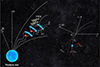 |
Fig. 1. Schematic diagram of a bulk of bunches moving in the magnetosphere is shown in the left panel. The light solid blue line shows the slice in which electrons emit roughly the same phase. The unit vector of the LOS is denoted as n, while ϵ1 and ϵ2 denote the two polarization components. The geometry for instantaneous circular motion for a particle identified by ijk in a bunch is on the right. The trajectory lies on the β0, ∥ − ϵ1 plane. At the retarded time, t = 0, the electron is at the origin. The dotted trajectory shows an electron at the origin. The angle between the solid and dotted trajectory is χij at t = 0. The angle between the LOS (z0) and the trajectory plane is φk. |
Inside a bunch, the total emission intensity is the summation of single charges that are coherently added. We considered a single charge that moves along a trajectory rs(t). The energy radiated per unit solid angle per unit frequency interval is interested in considering spectrum, which is given by (Rybicki & Lightman 1979; Jackson 1998):
![Mathematical equation: $$ \begin{aligned} \begin{aligned} \frac{\mathrm{d}^2W}{\mathrm{d}\omega \mathrm{d}\Omega }=&\frac{e^2\omega ^2}{4\pi ^2c}\\&\times \left|\int ^{+\infty }_{-\infty }\sum _{\rm s}^{N_{\rm s}} -\boldsymbol{\beta }_{\rm s\perp }\exp {[i\omega (t-\boldsymbol{n}\cdot \boldsymbol{r}_{\rm s}/c)]}\mathrm{d}t\right|^2, \end{aligned} \end{aligned} $$](/articles/aa/full_html/2024/05/aa48670-23/aa48670-23-eq2.gif) (2)
(2)
where βs⊥ is the component of βs in the plane that is perpendicular to the LOS:
 (3)
(3)
ϵ1 is the unit vector pointing to the center of the instantaneous circle, ϵ2 = n × ϵ1 is defined. If there is more than one charged particle, one can use subscripts (i, j, k) to describe any charge in the three-dimensional (3D) bunch. The subscripts contain all the information about the location. We assume that bunches are uniformly distributed in all directions of ( ). Equation (3) can be written as:
![Mathematical equation: $$ \begin{aligned} {\begin{aligned} \frac{\mathrm{d}^2W}{\mathrm{d}\omega \mathrm{d}\Omega }=&\frac{e^2 \omega ^2}{4 \pi ^2 c} \\&\times \left|\int _{-\infty }^{+\infty } \sum _i^{N_i} \sum _j^{N_j} \sum _k^{N_k}-\boldsymbol{\beta }_{i j k,\perp } \exp \left[i \omega \left(t-\boldsymbol{n} \cdot \boldsymbol{r}_{i j k}(t)/c\right)\right] \mathrm{d}t\right|^2, \end{aligned}} \end{aligned} $$](/articles/aa/full_html/2024/05/aa48670-23/aa48670-23-eq5.gif) (4)
(4)
where Ne = NiNjNk. The emission power from charges with the same phase is  enhanced. Detailed calculations are referred to Appendix A.
The bunches thus act like single macro charges in some respects. We define a critical frequency of curvature radiation, ωc = 3cγ3/(2ρ), where ρ is the curvature radius. Spectra of curvature radiation from a single charge can be described as a power law for ω ≪ ωc and exponentially drop when ω ≫ ωc. The spectrum and polarization properties of a bunch with a longitude size smaller than the half-wavelength and half-opening angle φt ≲ 1/γ, are similar to the case of a single charge. In general, the spectra can be characterized as multi-segmented broken power laws by considering a variety of geometric conditions of bunch (Yang & Zhang 2018; Wang et al. 2022a).
2.1.1. Bunch structure
There could be a lot of bunches contributing to instantaneous radiation in a moving bulk and their emissions are added incoherently. The spread angle of relativistic charge is:
 (5)
(5)
For ω ∼ ωc, bunches within a layer of ρ/γ can contribute to the observed luminosity at an epoch. The number of that contributing charges is estimated as  .
.
We assume that the number density in a bunch has ∂ne/∂t = 0. The case of fluctuating bunch density can give rise to a suppressed spectrum, and there is a quasi-white noise in a wider band in the frequency domain (Yang & Zhang 2023). The fluctuating density may cause the integral of Eq. (A.5) to not converge.
Different bunches may have different bulk Lorentz factors. We note that emissions from relativistic charges may have a characteristic frequency determined by the Lorentz factor. The scattering of the Lorentz factor from different emitting units likely enables the characteristic frequency to be polychromatic. Therefore, non-monoenergetic distributed charges give rise to a wide spectrum. However, for the bunch case discussed in Sect. 2, the layer contributing to the observed luminosity simultaneously is ∼ρ/γ much smaller than the curvature radius. Emission power in the layers is thus roughly the same. The Lorentz factors between different bunch layers can be regarded as a constant.
The frequency structure of a burst is essentially the Fourier transform of the spatial structure of the radiating charge density (Katz 2018). Therefore, a relatively narrow spectrum may be produced via the emission from a quasi-periodically structured bulk of bunches. The possible mechanisms that generate such a quasi-periodically structure are discussed in Sect. 3.
2.1.2. Spectrum of the bunch structure
We focus on the radiation properties due to the quasi-periodical structure. The charged bunch distribution is thought to be quasi-period in the time domain, which may be attributed to some quasi-periodic distribution in space between bunches. Each emitting bunch has the same E(t), but with different arrival times. The total received electric field from the multiple bunches simultaneously is given by:
 (6)
(6)
and its time-shifting property of the Fourier transform is:
 (7)
(7)
A quasi-periodically distributed bulk of bunches means that ωtn = nω/ωM + δϕn, where 1/ωM denotes the period of the bunch distribution and ϕn is the relative random phase.
A strictly periodically distributed bulk means that the relative random phase is zero strictly. The energy per unit time per unit solid angle is (Yang 2023):
![Mathematical equation: $$ \begin{aligned} \frac{\mathrm{d}^2W}{\mathrm{d}\omega \mathrm{d}\Omega }=c^2\mathcal{R} ^2\left|E_n(\omega )\right|^2\frac{\sin ^2[N_{\mathrm{b} }\omega /(2\omega _{\rm M})]}{\sin ^2[\omega /(2\omega _{\rm M})]}, \end{aligned} $$](/articles/aa/full_html/2024/05/aa48670-23/aa48670-23-eq11.gif) (8)
(8)
where ℛ is the distance from the emitting source to the observer. The coherence properties of the radiation by the multiple bulks of bunches are determined by ωM. The radiation is coherently enhanced when ω is 2πωM of integer multiples so that the energy is radiated into multiples of 2πωM with narrow bandwidths. Even when ϕn is not zero, the Monte Carlo simulation shows that the coherent radiation energy is still radiated into multiples of 2πωM with narrow bandwidths (Yang 2023).
Figure 2 shows the simulation of radiation spectra from quasi-periodically distributed bulk of bunches with ωM = 108 Hz and ωM = 5 × 10⁸ Hz. We assume that Nb = 104, γ = 102, δϕn = 0 and ρ = 107 cm. Since the flux drops to a small number rapidly when both 1/γ < φ′ and 1/γ < χ′, we fix χ′ = 10−3 in the simulations for simplicity. Spectra from uniformly distributed bulk of bunches are plotted as comparisons. By assuming there is an observation threshold exceeding the peak flux of the pure curvature radiation, the spectrum is characterized by multiple narrowband emissions with a bandwidth smaller than 2πωM. As ωM becomes larger, the number of spikes is smaller. Even though there are multi-spikes in the spectra, there is a main maximum at near ν = νc ordered larger than other spikes, so that multiple narrowband emissions are difficult to detect with an ultra-wideband receiver.
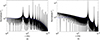 |
Fig. 2. Normalized spectra of the quasi-periodically structured bulk of bunches: (a) ωM = 108 Hz; (b) ωM = 5 × 10⁸ Hz. The black solid line is the spectrum due to the quasi-periodic structure. The blue dashed line is the spectrum of a uniformly distributed bulk of bunches. |
2.2. Perturbation on curved trajectories
We considered two general cases that the perturbations exist both parallel (E1, ∥) and perpendicular (E1, ⊥) to the local B-field independently. The perturbations can produce extra parallel  and perpendicular accelerations
  to the local B-field, as shown in Fig. 1. The perturbation electric fields are much smaller than the E∥, which is ∼107 esu, sustaining a constant Lorentz factor (Wang et al. 2019). When they are affected by these accelerations, electrons not only emit curvature radiation, but also emissions caused by the perturbations on the curved trajectory. As we have limited this issue to general discussion, we do not consider the perturbation in this section; instead, we simply require for the velocity to change slightly, namely, δβ ≪ β.
2.2.1. Parallel acceleration
The emission power by the acceleration parallel to the velocity, namely, longitudinal acceleration, is given by (Rybicki & Lightman 1979):
 (9)
(9)
According to Eq. (9), if the ratio of two longitudinal forces is N, the ratio of their emission power to N2, so that we can ignore the radiation damping caused by E1, ∥. The energy loss by radiation is mainly determined by the coherent curvature radiation. The balance between the E∥ and radiation damping is still satisfied approximately, leading to a constant Lorentz factor. Thus, the velocity change caused by E1, ∥ of a single charge can be described as:
 (10)
(10)
The velocity change is so slight that the partial integration of Eq. (A.5) converges, thus Eq. (A.6) can be obtained from Eq. (A.5).
2.2.2. Spectrum of parallel acceleration
The dimensionless velocity of a single charge reads βs = βs, 0 + β1, ∥, where βs, 0 is the mean dimensionless velocity and β1, ∥ is its perturbation parallel to the field lines, so that the emitting electric field can be calculated by the curvature radiation and perturbation-induced emission independently. Let us consider a charge with a dentifier of i, j, k in a bunch. The polarization components of the parallel perturbation-induced wave are calculated as:
![Mathematical equation: $$ \begin{aligned} \begin{aligned} \tilde{A}_{ijk,\Vert }\simeq &\int ^{+\infty }_{-\infty }\beta _{1,\Vert } (t)\sin \left(\frac{ct}{\rho }+\chi _{ij}\right)\\&\times \exp \left(i \frac{\omega }{2}\left[\left(\frac{1}{\gamma ^{2}}+\varphi _k^{2}+\chi _{ij}^{2}\right) t+\frac{c^{2} t^{3}}{3 \rho ^{2}}+\frac{c t^{2}}{\rho } \chi _{ij}\right]\right)\mathrm{d}t,\\ \tilde{A}_{ijk,\perp }\simeq &\int ^{+\infty }_{-\infty } \beta _{1,\Vert }(t)\sin \varphi _k\cos \left(\frac{ct}{\rho }+\chi _{ij}\right)\\&\times \exp \left(i \frac{\omega }{2}\left[\left(\frac{1}{\gamma ^{2}}+\varphi _k^{2}+\chi _{ij}^{2}\right) t+\frac{c^{2} t^{3}}{3 \rho ^{2}}+\frac{c t^{2}}{\rho } \chi _{ij}\right]\right)\mathrm{d}t.\\ \end{aligned} \end{aligned} $$](/articles/aa/full_html/2024/05/aa48670-23/aa48670-23-eq16.gif) (11)
(11)
A complex spectrum can be caused by a complexly varying β1, ∥(t). A simple case is that the integrals of Eq. (11) can be described by the modified Bessel function Kν(ξ) if β1 is a constant. The function is approximated to be power-law-like for ξ ≪ 1 and exponential-like for ξ ≫ 1, when ν ≠ 0. Here, it is worth noting that Kν(ξ = 0)→+∞ when ξ = 0, exhibiting a very narrow spectrum.
In particular, if a waveform E(t) is quasi-sinusoid periodic, the spectrum would be quasi-monochromatic, equivalently to the narrowband. The quasi-sinusoid periodic waveform can be produced by the intrinsic charge radiation if the charge is under a periodic acceleration during its radiation beam pointing to the observer. For a perturbation E1.∥, which is monochromatic oscillating with time of interest, according to Eq. (A.1), the velocity is also monochromatic oscillating. Therefore, we introduce a velocity form with monochromatic oscillating in the lab frame, that is, β1, ∥(t) = β1exp(−iωat). The two parameters introduced in the curvature radiation in Eq. (A.11) are replaced by:
 (12)
(12)
The radiation can be narrowband when γ is a constant and the center frequency is:
 (13)
(13)
For the bunching emission, charges are located with different χ and φ, which results in the bandwidth getting wider. Now we consider the change in the value of E∥ is much smaller than l∂E∥/∂r ≪ E∥, where l is the longitude bunch size. The charges in the bunch are then monoenergic. However, for an ultra-relativistic particle, a small change in velocity can create a violent change in the Lorentz factor, namely, δγ ≃ γ3βδβ∥. To keep the electrons monoenergic, it is required for the amplitude to be β1 ≪ 1/γ2.
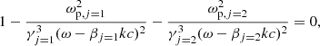
Following the Appendix A, one can obtain the spectrum of bunching charges. Adopting γ = 100, ρ = 107 cm, φ = 0, and ωa = 2π × 105 Hz, we simulate the spectra in four cases: φt = 0.1/γ, β1 = 10−6; φt = 0.1/γ, β1 = 10−5; φt = 1/γ, β1 = 10−6; and φt = 1/γ, β1 = 10−5, shown as Fig. 3. The spectra are normalized to the Fν of curvature radiation with φt = 10−3 at ω = ωc. For φt = 0.1/γ, the spectra show spikes at 2νaγ2. The amplitude of spikes decreases as β1 decreases. For φt = 1/γ, the scattering of φ′ leads the spikes to become wider and shorter. The small amplitude β1 allows for the spike disappear and the spectrum is then determined by the curvature radiation. As φ becomes larger, more different trajectories may have more different azimuths so that the coherence of emission decreases. The spectrum has a flat component at ω < ωc when 3c/ρ < ωc(χ′2 + φ′2)3/2 (Yang & Zhang 2018).
 |
Fig. 3. Normalized spectra of the parallel perturbation cases at φ = 0: φt = 0.1/γ, β1 = 10−6 (blue dashed line); φt = 0.1/γ, β1 = 10−5 (red dotted line); φt = 1/γ, β1 = 10−6 (black solid line); and φt = 1/γ, β1 = 10−5 (green dashed-dotted line). |
2.2.3. Perpendicular acceleration
For a comparable parallel and perpendicular forces, dp/dt, the radiation power from the parallel component is on the order of 1/γ2 compared to that from the perpendicular component. The energy loss by radiation is also mainly determined by the coherent curvature radiation. Similar to the parallel scenario, the velocity change caused by E1, ⊥ of a single charge can be described as:
 (14)
(14)
when β1, ⊥ ≪ β∥. The velocity change is also slight, therefore, we can use Eq. (A.6) to calculate the spectrum (see Appendix A).
2.2.4. Spectrum of perpendicular acceleration
The polarization components of the perpendicular perturbation-induced wave of a charge with an identifier of ijk are calculated as:
![Mathematical equation: $$ \begin{aligned} \begin{aligned} \tilde{A}_{ijk,\Vert }\simeq &\int ^{+\infty }_{-\infty }\frac{1}{2} \beta _{1,\perp }(t)\left[\varphi _k^2-(\chi _{ij}+ct/\rho )^2\right]\\&\times \exp \left(i \frac{\omega }{2}\left[\left(\frac{1}{\gamma ^{2}} +\varphi _k^{2}+\chi _{ij}^{2}\right) t+\frac{c^{2} t^{3}}{3 \rho ^{2}} +\frac{c t^{2}}{\rho } \chi _{ij}\right]\right)\mathrm{d}t,\\ \tilde{A}_{ijk,\perp }\simeq &\int ^{+\infty }_{-\infty }\beta _{1,\perp } (t)\varphi _k (\chi _{ij}+ct/\rho ) \\&\times \exp \left(i \frac{\omega }{2}\left[\left(\frac{1}{\gamma ^{2}} +\varphi _k^{2}+\chi _{ij}^{2}\right) t+\frac{c^{2} t^{3}}{3 \rho ^{2}} +\frac{c t^{2}}{\rho } \chi _{ij}\right]\right)\mathrm{d}t,\\ \end{aligned} \end{aligned} $$](/articles/aa/full_html/2024/05/aa48670-23/aa48670-23-eq20.gif) (15)
(15)
where χij and φk are small angles. The amplitudes are much smaller than those of parallel perturbations with comparable β1. Similar to the parallel scenario, the total amplitudes of a bunch for the perpendicular perturbation case can be calculated by summation of Eq. (A.17).
A narrow spectrum is expected when γ is a constant with the scattering of χ and φ is small. The spike is at ω = 2γ2ωa resembling that of the parallel perturbation case. A small change in velocity can also make a violent change in the Lorentz factor but with a noticeable difference from that of longitude motion. Under the energy supply from the E∥, charges have β∥ ≈ 1. The change in the Lorentz factor is δγ ≃ γ3β⊥δβ⊥ when β1, ⊥ ≪ 1. To keep electrons being monoenergic, the condition of β1 ≪ 1/γ should be satisfied at least.
Following the calculation steps in the Appendix A, we simulate the spectra in four cases: φt = 0.1/γ, β1 = 10−4; φt = 0.1/γ, β1 = 10−3; φt = 1/γ, β1 = 10−4; and φt = 1/γ, β1 = 10−3, shown as Fig. 4. Here, we take γ = 100, ρ = 107 cm, φ = 0 and ωa = 2π × 105 Hz. The spectra are normalized to the Fν of curvature radiation with φt = 10−3 at ω = ωc. The spikes for the four cases are very small so the spectra are dominated by curvature radiations.
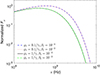 |
Fig. 4. Normalized spectra of the perpendicular perturbation cases at φ = 0: φt = 0.1/γ, β1 = 10−4 (blue dashed line); φt = 0.1/γ, β1 = 10−3 (red dotted line); φt = 1/γ, β1 = 10−4 (black solid line); and φt = 1/γ, β1 = 10−3 (green dashed-dotted line). |
2.3. Polarization of the intrinsic radiation mechanisms
Four Stokes parameters can be used to describe the polarization properties of a quasi-monochromatic electromagnetic wave (see Appendix B). Based on Eq. (A.6), the electric vectors of the emitting wave reflect the motion of charge in a plane normal to the LOS. For instance, if the LOS is located within the trajectory plane of the single charge, the observer will see electrons moving in a straight line so that the emission is 100% linearly polarized. Elliptical polarization would be seen if the LOS is not confined to the trajectory plane. We define that φ < θc as on-beam and φ > θc as off-beam. For the bunch case, similar on-beam and off-beam cases can also be defined in which θc is replaced by φt + θc (Wang et al. 2022b). The general conclusion of the bunching curvature radiation is that high linear polarization appears for the on-beam geometry, whereas high circular polarization is present for the off-beam geometry.
We consider the polarization properties of the bunch structure case (Sect. 2.1.2), and the perturbation scenarios including the parallel and the perpendicular cases (Sect. 2.2). For the quasi-periodically distributed bulk of bunches scenario, both A∥ and A⊥ are multiplied by the same factor, so that the polarization properties are similar with a bulk of bunches, which bunches are uniformly distributed (e.g., Wang et al. 2022a). For the perturbation scenario, the perturbation on the curved trajectory can bring new polarization components, which generally obey the on(off)-beam geometry. However, the intensity of the perturbation-induced components is too small then the polarization profiles are mainly determined by the bunching curvature radiation. Consequently, the polarization properties for both the bunching mechanism and the perturbation scenarios can be described by the uniformly distributed bulk of bunches.
We took γ = 102, φt = 10−2 and ρ = 107 cm. The beam angle at ω = ωc is 0.02. According to the calculations in Appendix B, we simulate the I, L, V, and PA profiles, shown in Fig. 5. These four parameters can completely describe all the Stokes parameters. The total polarization fraction is 100% because the electric vectors are coherently added. The polarization position angle (PA) for the linear polarization exhibits some variations but within 30°. The differential of V is the largest at φ = 0 and becomes smaller when |φ| gets larger. A high circular polarization with flat fractions envelope would appear at off-beam geometry. In this case, the flux is smaller but may still be up to the same magnitude as the peak of the profile (e.g., Liu et al. 2023b). The spectrum at the side of the beam becomes flatter due to the Doppler effect (Zhang 2021). The sign change in the V would be seen when φ = 0 is confined into the observation window (Wang et al. 2022b).
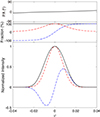 |
Fig. 5. Simulated polarization profiles for the bunch with γ = 102, φt = 10−2, ρ = 107 cm. Top panel: polarization position angle envelope. Middle panel: total polarization fraction (black solid line), linear polarization fraction (red dashed line), and circular polarization fraction (blue dashed-dotted line). Bottom: total intensity, I, (black solid line), linear polarization, L, (red dashed line), and circular polarization, V, (blue dashed-dotted line) as functions of φ. All three functions are normalized to the value of I at φ = 0. |
3. Trigger of bunches
The trigger mechanism plays an important role in producing bunching charges and creating the E∥. Intriguingly, a giant glitch was measured 3.1 ± 2.5 days before FRB 20200428A associated with a quasi-periodic oscillations (QPOs) of ∼40 Hz in the X-ray burst from the magnetar SGR J1935+2154 (Mereghetti et al. 2020; Li et al. 2021, 2022; Ridnaia et al. 2021; Tavani et al. 2021; Ge et al. 2022). Another glitch event was found on October 5, 2020 and the magnetar emitted three FRB-like radio bursts in subsequent days (Younes et al. 2023; Zhu et al. 2023). Both the glitches and QPOs are most likely the smoking guns of starquakes. Therefore, magnetar quakes are considered a promising trigger model of FRB in the following.
As discussed in Sect. 2.1.2, we are particularly interested in the mechanisms that can generate quasi-periodically distributed bunches. Two possible scenarios are discussed independently in Sects. 3.1.1 and 3.1.2. Motivated by the fact that Alfvén waves associated with the quake process have been proposed by lots of models (e.g., Wang et al. 2018; Kumar & Bošnjak 2020; Yang & Zhang 2021; Yuan et al. 2022), we discuss the Alfvén waves as the perturbations in Sect. 2.2.
3.1. Structured bunch generation
3.1.1. Pair cascades from the “gap”
A magnetized neutron star’s rotation can create a strong electric field that extracts electrons from the stellar surface and accelerates them to high speeds (Ruderman & Sutherland 1975). The induced electric field region lacks adequate plasma, namely, charge-starvation, referred to as a “gap”. The extracted electrons move along the curved magnetic field lines near the surface, emitting gamma rays absorbed by the pulsar’s magnetic field, resulting in electron-positron pairs. Such charged particles then emit photons that exceed the threshold for effective pair creation, resulting in pair cascades that populate the magnetosphere with secondary pairs. The electric field in the charge-starvation region is screened once the pair plasma is much enough and the plasma generation stops (Levinson et al. 2005). When the plasma leaves the region, a gap with almost no particles inside is formed forms again and the vacuum electric field is no longer screened.
The numerical simulations show that such pair creation is quasi-periodic (Timokhin 2010; Tolman et al. 2022), leading to quasi-periodically distributed bunches. The periodicity of cascades is ∼3 hgap/c, where hgap is the height of the gap. The gap’s height is expressed as (Timokhin & Harding 2015):
 (16)
(16)
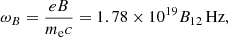
where P is the spin period and α is the inclination angle of magnetic axis. For a typical radio pulsar, we take B = 1012 G and P = 1 s. The corresponding ωM is 107 Hz. According to Eq. (8), radiation energy is emitted into multiples of ∼10 MHz narrow bandwidths, which is consistent with the narrowband drifting structure of PSR B0950+08 (Bilous et al. 2022).
In contrast to the continuous sparking in the polar cap region of normal pulsars, FRB models prefer a sudden, violent sparking process. Starquake as a promising trigger mechanism can occur when the pressure induced by the internal magnetic field exceeds a threshold stress. The elastic and magnetic energy released from the crust into the magnetosphere are much higher than the spin-down energy for magnetars. Crust shear and motion may create hills on the surface. The height of the gap becomes smaller and the electric field is enhanced due to the so-called point-discharging. Quasi-periodically distributed bunches with ωM ∼ 108 may be formed from such shorter gaps. Observational consequences of small hills on stellar surfaces could also be known by studying regular pulsars (e.g., Wang et al. 2023).
We note that the sparking process to generate FRB-emitting bunches is powered by magnetic energy, rather than spin-down energy. The stellar oscillations during starquakes can provide additional voltage, making the star active via sparking (Lin et al. 2015). The oscillation-driven sparking process may generate much more charges than the spin-down powered sparking of a normal rotation-powered pulsar.
3.1.2. Two-stream Instability
Alternatively, another possibility to form charged bunches is the two-stream instability between electron-positron pairs. The growth rate of two-stream instability is discussed by invoking linear waves. Following some previous works (e.g., Usov 1987; Gedalin et al. 2002; Yang & Zhang 2023), we consider that there are two plasma components denoted as “1” and “2” with a relative motion along the magnetic field line. The Lorentz factor and the particle number density are γj and nj with j = 1, 2. Each plasma component is assumed to be cold in the rest frame of each component. Then the dispersion relation of the plasma could be written as (Asseo & Melikidze 1998):
 (17)
(17)
where ωp, j is the plasma frequency of the component j. For the resonant reactive instability as the bunching mechanism, the growth rate and the characteristic frequency of the Langmuir wave are given by (e.g., Usov 1987; Gedalin et al. 2002; Yang & Zhang 2023):
 (18)
(18)
 (19)
(19)
The linear amplitude of the Langmuir wave depends on the gain, G ∼ Γr/c. According to Rahaman et al. (2020), a threshold gain, Gth, indicating the breakdown of the linear regime is about Gth ∼ a few. The sufficient amplification would drive the plasma beyond the linear regime once G ∼ Gth, and the bunch formation rate is Γ(G ∼ Gth). The bunch separation corresponds to the wavelength of the Langmuir wave for G ∼ Gth, namely,
 (20)
(20)
A narrowband spectrum with Δν ∼ 100 MHz would be created if  Hz.
Hz.
Generally, the charged bunches would form and disperse dynamically due to the instability, charge repulsion, velocity dispersion, and so on (e.g., Lyutikov 2021; Yang & Zhang 2023). The spectrum of the fluctuating bunches depends on the bunch formation rate, λB, lifetime, τB, and bunch Lorentz factor, γ, as proposed by Yang & Zhang (2023). The coherent spectrum by a fluctuating bunch is suppressed by a factor of (λBτB)2 compared with that of a persistent bunch and there is a quasi-white noise in a wider band in the frequency domain. The observed narrow spectrum implies that, at the minimum, the quasi-white noise should not be dominated in the spectrum, in which case, the condition of 2γ2λB ≳ min(ωpeak, 2γ2/τB) would be required, where ωpeak is the peak frequency of curvature radiation. We refer to Yang & Zhang (2023) for a detailed discussion.
3.2. Quake-induced oscillation and Alfvén waves
An Alfvén wave packet can be launched from the stellar surface during a sudden crustal motion and starquake. The wave vector is not exactly parallel to the field line so the Alfvén waves have a non-zero electric current along the magnetic field lines. Starquakes as triggers of FRBs are always accompanied by Alfvén wave launching. We investigate whether Alfvén waves as the perturbations discussed in Sect. 2.2 can affect the spectrum.
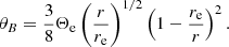
The angular frequencies of the torsional modes Ω caused by a quake are calculated as follows (also see Appendix C). We chose the equation of state (EOS A; Pandharipande 1971) and EOS WFF3 (Wiringa et al. 1988), which describe the core of neutron stars, as well as to consider two different proposed EOSs for the crusts, including EOSs for NV (Negele & Vautherin 1973) and DH (Douchin & Haensel 2001) models. We match the various core EOS to two different EOSs for the crust. The crust-core boundary for the NV and DH EOSs is defined at ρm ≈ 2.4 × 10¹⁴ g cm−3, and ρm ≈ 1.28 × 10¹⁴ g cm−3, respectively.
The frequencies of torsional modes are various with a strong magnetic field (Messios et al. 2001). As already emphasized by Sotani et al. (2007), the shift in the frequencies would be significant when the magnetic field exceeds ∼1015 G. In the presence of magnetic fields, frequencies are shifted as:
![Mathematical equation: $$ \begin{aligned} _\ell f_n = _\ell f_n^{(0)} \left[1+ _\ell \alpha _n \left(\frac{B}{B_{\mu }}\right)^2 \right]^{1/2}, \end{aligned} $$](/articles/aa/full_html/2024/05/aa48670-23/aa48670-23-eq27.gif) (21)
(21)
where ℓαn is a coefficient depending on the structure of the star,  is the frequency of the non-magnetized star, and Bμ ≡ (4πμ)1/2 is the typical magnetic field strength.
In Fig. 6, we show the effects of the magnetic field on the frequencies of the torsional modes. The magnetic field strength is normalized by Bμ = 4 × 10¹⁵ G. Different dashed lines in Fig. 6 are our fits to the calculated numerical data with a high accuracy. For B > Bμ, we find that the frequencies follow a quadratic increase against the magnetic field, and tend to become less sensitive to the NS parameters. The oscillation frequencies exceed 103 Hz for n = 2 and Ω ∼ 104 Hz for typical magnetars.
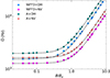 |
Fig. 6. Frequencies of the second overtone n = 2 and ℓ = 2 torsional modes as a function of the normalized magnetic field (B/Bμ). The NS mass is M = 1.4 M⊙. The dashed lines correspond to our fits using the empirical formula (21) with different coefficient values. The fitting values are 2.4, 0.78, 2.2, and 0.69 for WFF3+ DH model, WFF3+ NV model, A+ DH model, and A+ NV model, respectively. |
Alfvén waves are launched from the surface at a frequency of Ω, which is much faster than the angular frequency of the spin, and propagate along the magnetic field lines. Modifying the Goldreich-Julian density can produce electric fields to accelerate magnetospheric charged particles. The charged particles oscillate at the same frequency as the Alfvén waves in the comoving frame. In the lab frame, the perturbation has  due to the Doppler effect, where
  . ωa is much smaller than
  Hz because of the strong magnetic field and low mass density in the magnetosphere.
Therefore, by considering that Alfvén waves play a role in the electric perturbations discussed in Sect. 2.2, the spectra have no spike from 100 MHz to 10 GHz, which is the observation bands for FRBs so far. The spectral spike would appear at the observation bands when the perturbations are global oscillations, meaning that all positions in the magnetosphere oscillate simultaneously with Ω rather than a local Alfvén wave packet.
4. Absorption effects in the magnetosphere
In this section, we investigate absorption effects during the wave propagating the magnetosphere. The absorption effects that have been discussed as a possible origin for the narrowband emission are independent of the intrinsic mechanisms in Sect. 2. To create narrowband emission, there must be a steep frequency cut-off on the spectrum that is due to the absorption conditions. Absorption conditions should also change cooperatively with the emission region, that is, the cut-off would appear at a lower frequency as the flux peak occurs at a lower frequency. Curvature radiation spectra can be characterized as a power law for ω < ωc and exponential function at ω > ωc (Jackson 1998). In the following discussion, we mainly consider two absorption mechanisms including Landau damping and self-absorption of curvature radiation.
4.1. Wave modes
Here, we consider the propagation of electromagnetic waves in magnetospheric relativistic plasma. The magnetosphere mainly consists of relativistic electron-positron pair plasma, which can affect the radiation created in the inner region. We assume that the wavelength is much smaller than the scale lengths of the plasma and of the magnetic field in which the plasma is immersed. The scale lengths of the magnetic field can be estimated as B/(∂B/∂r)∼r. The plasma is consecutive and its number density is thought to be multiples of the Goldreich-Julian density (Goldreich & Julian 1969), leading to the same scale lengths as that of the magnetic field. Both the scale lengths of magnetic field and plasma are much larger than the wavelength  cm, even for the outer magnetosphere at r ∼ 4.8 × 10⁹P0 cm.
No matter whether it is a neutron star or a magnetar, the magnetospheric plasma is highly magnetized. It is useful to define the (non-relativistic) cyclotron frequency and plasma frequency:
 (22)
(22)
 (23)
(23)
where np = ℳnGJ = ℳB/(ceP), in which nGJ is the Goldreich-Julian density and ℳ is a multiplicity factor. In the polar-cap region of a pulsar, a field-aligned electric field may accelerate primary particles to ultra-relativistic speed. The pair cascading may generate a lot of plasma with lower energy and a multiplicity factor of ℳ ∼ 102 − 105 (Daugherty & Harding 1982). The relationships ω ≪ ωB and ωp ≪ ωB are satisfied at most regions inside the magnetosphere.
The vacuum polarization may occur at the magnetosphere for high energy photons and radio waves by the plasma effect in a strong magnetic field (Adler 1971). In the region of r ≳ 10 R, where FRBs can be generated, in which R is the stellar radius, the magnetic field strength  with assumption of Bs = 1015 at stellar surface. In the low-frequency limit ℏω ≪ mec2, the vacuum polarization coefficient can be calculated as
  (Heyl & Hernquist 1997; Wang & Lai 2007). Therefore, the vacuum polarization can be neglected in the following discussion about the dispersion relationship in the magnetosphere.
Waves have two propagation modes: O-mode and X-mode. In the highly magnetized relativistic case, the dispersion of X-mode photon is n ≈ 1. O-mode photons have two branches in the dispersion relationship, which are called subluminous O-mode (n > 1) and superluminous O-mode (n < 1), shown as Fig. D.1. The subluminous O-mode cuts off at 1/cosθB, where θB is the angle between angle between  and
and  . Following the calculation shown in Appendix D, the dispersion relation of magnetospheric plasma for subluminous O-mode photons can be found following (Arons & Barnard 1986; Beskin et al. 1988):
 (24)
(24)
with
![Mathematical equation: $$ \begin{aligned} g_{\rm s}=\mathcal{P} \int _{-\infty }^{\infty } \frac{f(u)\mathrm{d}u}{\gamma ^3\left(1-n_{\Vert } \beta \right)^2}+i \pi \beta _n^2\gamma _n^3 \left[\frac{\mathrm{d}f}{\mathrm{d}u}\right]_{\beta =\beta _n}, \end{aligned} $$](/articles/aa/full_html/2024/05/aa48670-23/aa48670-23-eq40.gif) (25)
(25)
where  ,
,  and f(u) is the distribution function of plasma.
4.2. Landau damping
Wave forces can exist many collective waves in a beam and exchange energy between waves and particles. If the distribution function is df/dv < 0 close to the phase speed of the wave, the number of particles with speeds v < ω/k will be larger than that of the particles having v > ω/k. Then, the transmission of energy to the wave is then smaller than that absorbed from the wave, leading to a Landau damping of the wave. According to the dispersion relationship given in Sect. 4.1, there is no linear damping of the X-mode since wave-particle resonance is absent. The superluminous branch of the O-mode also has no Landau damping because the phase speed exceeds the speed of light. Landau damping only occurs at the subluminous O-mode photons.
The Landau damping decrement can be calculated by the imaginary part of the dispersion relationship (Boyd & Sanderson 2003). We let k = kr + iki, where ki ≪ kr ≈ k. If a wave has a form of E ∝ exp(−iωt + ikr), the imaginary ki can make the amplitude drop exponentially. The imaginary part of Eq. (24) by considering a complex waveform of k is given by:
 (26)
(26)
where gr and gi denote the real and imaginary parts of Eq. (25). We consider the emission at a radius, re, along a field line whose footprint intersects the crust at magnetic colatitude Θe(R/re)1/2 for Θe ≪ 1, one can obtain the angle between k and B at each point:
 (27)
(27)
Consequently, the optical depth for waves emitted at re to reach r is:
 (28)
(28)
Even the distribution function for the magnetospheric electrons and positrons is not known, a relativistic thermal distribution is one choice. Since the vertical momentum drops to zero rapidly, for instance, a 1D Jüttner distribution is proposed here (e.g., Melrose et al. 1999; Rafat et al. 2019):
 (29)
(29)
where ρT = mec2/(kBT), in which T is the temperature of plasma and kB is the Boltzmann constant. Alternatively, another widely used distribution is a Gaussian distribution (e.g., Egorenkov et al. 1983; Asseo & Melikidze 1998):
 (30)
(30)
where um can be interpreted as the average u over the distribution function. Besides a thermal distribution, power law distributions  , where p is the power law index (p > 2), are representative choice to describe the plasma in the magnetosphere (e.g., Kaplan & Tsytovich 1973).
The optical depths as a function of wave frequency with four different distributions are shown in Fig. 7. Here, we assume that re = 107 cm, ℳ = 103, γp = 10 and Θe = 0.05. For all considered distributions, optical depths decrease with frequencies which means that the Landau damping is more significant for lower-frequency subluminous O-mode photons. The optical depths are much larger than 1 for the FRB emission band so that the subluminous O-mode photon cannot escape from the magnetosphere. Superluminous O-mode photons which frequency higher than 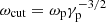 can propagate. The bunching curvature radiation is exponentially dropped at ω > ωc. If the superluminous O-mode cut-off frequency is close to ωc, the spectrum of the emission would be narrow. A simple condition could be given when a dipole field is assumed:
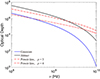 |
Fig. 7. Optical depths for four distributions: Jüttner with ρT = 0.1 (black solid line), Gaussian with |
 (31)
(31)
where the emission region is considered at closed field lines in which ρ ∼ r. The cut-off frequency ωcut ∝ r−3/2 which evolves steeper than ωc ∝ r−1. The bandwidth is suggested to become wider as the burst frequency gets lower.
Coherent curvature radiation can propagate out of the magnetosphere via superluminous O-mode with a frequency cut-off, which likely leads to narrow spectra. However, the condition that the frequency cut-off is close to the characteristic frequency of curvature radiation could not be satisfied at all heights, leading to narrow spectra sometimes. The waves can also propagate via X-mode photon which has no frequency cut-off. The spectrum of X-mode photons ought to be broad. The waves propagate via whether X-mode or O-mode is hard to know because the real magnetic configuration is complex. Narrow spectra have been found in some FRBs, while some FRBs seem to have broad spectra and there are also some not sure due to the limitation of bandwidth of the receiver (Zhang et al. 2023).
In principle, the spectrum of a radio magnetar would be narrow, if the emission is generated from r > 10 R propagating via O-mode. However, radio pulses are rarely detected among magnetars. For normal pulsars, the lower magnetic fields may induce lower number density so that the Landau damping is not as strong as in magnetars.
4.3. Self-absorption by curvature radiation
The self-absorption is also associated with the emission. We assume that the momentum of the particle is still along the magnetic field line even after having absorbed the photon. The cross-section can be obtained through the Einstein coefficients when hν ≪ γsmec2 (e.g., Locatelli & Ghisellini 2018):
![Mathematical equation: $$ \begin{aligned} \frac{\mathrm{d} \sigma _{\mathrm{c} }}{\mathrm{d} \Omega } = \frac{1}{2 m_{\mathrm{e} } \nu ^2} \frac{\partial }{\partial \gamma _{\rm s}}\left[j_{\rm s}(\nu , \gamma _{\rm s}, \varphi _{\rm s})\right], \end{aligned} $$](/articles/aa/full_html/2024/05/aa48670-23/aa48670-23-eq52.gif) (32)
(32)
where σc is the curvature cross section and js is the emissivity.
There are special cases which the stimulated emission becomes larger than the true absorption. As a result, the total cross section becomes negative, and there is a possible maser mechanism. However, such maser action is ineffective when the magnetic energy density is much higher than that for the kinetic energy of charges (Zhelezniakov & Shaposhnikov 1979). The isotropic equivalent luminosity for the curvature radiation is ∼1042 erg s−1 if Ne = 1022 at r = 107 cm for γ = 102 (Kumar et al. 2017). The number density in a bunch is estimated as ne ∼ 1011 cm−3 by Wang et al. (2022a), so that neγmec2 ≪ B2/(8π). Thus, the maser process is ignored in the following discussion.
By inserting the curvature power per unit frequency (see e.g., Jackson 1998), the total cross section integrated over angles is given by Ghisellini & Locatelli (2018):
 (33)
(33)
where Γ(ν) is the gamma function. As explained in the discussion in Sect. 2, the charges are approximately monoenergetic due to the rapid balance between E∥ and the curvature damping. The absorption optical depth is:
 (34)
(34)
The absorption is more significant for lower frequencies.
Figure 8 exhibits the comparison between purely bunching curvature radiation and it after the absorption. We adopt that γs = 102, ne = 1011 cm−3 and ρ = 107 cm. The plotted spectra are normalized to the Fν of curvature radiation with φt = 10−3 at ω = ωc. The spectral index is 5/3 at lower frequencies due to the self-absorption, which is steeper than pure curvature radiation, but it is still wide-band emission. Alternatively, the E∥ can let electrons and positrons decouple, which leads to a spectral index of 8/3 at lower frequencies (Yang et al. 2020). The total results of these independent processes can make a steeper spectrum, with an index of 13/3.
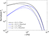 |
Fig. 8. Normalized spectra of self-absorbed curvature radiation. Black lines denote purely bunching curvature radiations for φt = 0.1/γ (solid line) and φt = 1/γ (dashed-dotted line). Blue lines denote the radiation after curvature self-absorption for φt = 0.1/γ (solid line) and φt = 1/γ (dashed-dotted line). |
5. Bunch expansion
As the bunch moves to a higher altitude, the thickness of the bunch (the size parallel to the field lines) becomes larger due to the repulsive force of the same sign charge. If the bunch travels through the emission region faster than the LOS sweeps across the whole emission beam, the thickness can be estimated as cw, where w is the burst width (Wang et al. 2022b). For simplicity, we consider the motion of electrons at the boundary due to the Coulomb force from bunches in the co-moving rest frame. The acceleration of an electron at the boundary is estimated as:
 (35)
(35)
where  is the transverse size of bunch. We note that the transverse size of a bunch is much larger than the longitude size even in the co-moving rest frame. Equation (35) is then calculated as
  . Charged particles in the bunch cannot move across the B-field due to the fast cyclotron cooling. The transverse size is essentially Rb ∝ r due to the magnetic freezing, thus, we have
  . The distance that the electron travels in the co-moving frame is s′∝r by assuming r ≫ r0 (r0 is an initial distance). As a result, the thickness of the bunch is cw ∝ r in the lab frame.
A burst width, w, would be larger if the emission is seen from a higher altitude region. If there is more than one bulk of bunches being observed coincidentally but with different trajectory planes, we would see the drifting pattern (Wang et al. 2019). The geometric time delay always lets a burst from a lower region be seen earlier, that is, a downward drifting pattern is observed. A subpulse structure with such a drifting pattern is a natural consequence caused by the geometric effect when the characteristic frequency of the emission is height-dependent.
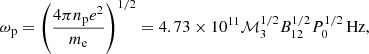
Following the previous work (Wang et al. 2022a), we continuously investigate the drifting rate as a function of the burst central frequency and width. The drift pattern is a consequence of narrowband emission. Compared with our previous work, we add the fitting results of FRB 20180916B. Figures 9 and 10 show the best fitting results for FRB 20121102A (blue dashed-dotted lines), FRB 20180916B (red dashed lines) and all FRBs (black solid lines) and their corresponding 1σ regions. The best fitting of  relationship for FRB 20121102A, FRB 20180916B, and all FRBs are
  ,
,  , and
, and  . The best fitting of
  as a function of ν/width for FRB 20121102A, FRB 20180916B and all FRBs are
  ,
,  , and
, and  . The fitting results generally match the case of curvature radiation, which has
  . The relationship
  is attributed to w ∝ r. Data are quoted from references as follows: Michilli et al. (2018), Gajjar et al. (2018), Hessels et al. (2019), Josephy et al. (2019), Caleb et al. (2020), Platts et al. (2021), Kumar et al. (2023), CHIME/FRB Collaboration (2019b, 2020b), Chamma et al. (2021), Chawla et al. (2020), Pastor-Marazuela et al. (2021), Sand et al. (2022), Day et al. (2020), Hilmarsson et al. (2021), Zhou et al. (2022), Gopinath et al. (2024).
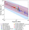 |
Fig. 9. Comparison of drift rates at different frequencies. Different regions show the 1σ region of the best fitting results: FRB 20121102A (blue), FRB 180916B(red), and all FRBs (grey). |
6. Discussion
6.1. Curvature radiation
The curvature radiation is formed since the perpendicular acceleration on the curved trajectory and its spectrum is naturally wide-band. Spectra of bunching curvature radiation are more complex due to the geometric conditions and energy distribution (e.g., Yang & Zhang 2018; Wang et al. 2022a). Despite considering the complex electron energy distributions, it remains challenging for the spectrum to appear in the narrowband.
However, quasi-periodically distributed bunches are able to create such narrowband emission. The radiation from the bulk of bunches is quasi-periodically enhanced and the bandwidth depends on ωM and the threshold of the telescope. As shown in Fig. 2, narrowband emissions with roughly the same bandwidth are expected to be seen from multi-band observations simultaneously. The energy is radiated into several multiples of 2πωM with narrow bandwidths and the required number of particles in the bunch is smaller than that of pure curvature radiation.
6.2. Inverse Compton scattering
Inverse Compton scattering (ICS) occurs when low-frequency electromagnetic waves enter bunches of relativistic particles (Zhang 2022). The bunched particles are induced to oscillate at the same frequency in the comoving frame. The outgoing ICS frequency in the lab frame is calculated as:
 (36)
(36)
where ωin is the angular frequency of the incoming wave and θin is the angle between the incident photon momentum and the electron momentum. This ICS process could produce a narrow spectrum for a single electron by giving a low-frequency wave of narrow spectrum (Zhang 2023). In order to generate GHz waves, dozens of kHz incoming wave is required for bunches with γ = 102 and θin should be larger than 0.5. This requires the low-frequency waves to be triggered from a location very far from the emission region. The X-mode of these waves could propagate freely in the magnetosphere, but O-mode would not be able to unless the propagation path of the waves approaches a vacuum-like environment.
As discussed in Sect. 2, the Lorentz factor is constant due to the balance between E∥ and radiation damping. θin varies slightly as the LOS sweeps across different field lines. If the incoming wave is monochromatic, the outgoing ICS wave would have a narrow value range matching the observed narrow-band FRB emissions. The polarization of ICS from a single charge is strongly linearly polarized, however, the electric complex vectors of the scattered waves in the same direction are added for all the particles in a bunch. Therefore, circular polarization would be seen for off-beam geometry (Qu & Zhang 2023), similar to the case of bunching curvature radiation but they are essentially different mechanisms (Wang et al. 2022c). Doppler effects may be significant at off-beam geometry so that the burst duration and spectral bandwidth would get larger. The model predicts that a burst with higher circular polarization components tends to have wider spectral bandwidth. This may differ from the quasi-periodically distributed bunch case, in which the mechanism to create narrow spectra is independent of polarization.
The perturbation discussed in Sect. 2.2 can let charges oscillate at the same frequency in the comoving frame. This process is essentially the same as the ICS emission. The acceleration caused by the perturbation is proposed to be proportional to exp(−iωat), which leads to the wave frequency of ωa(1 − βcosθin) due to the Doppler effect in the lab frame. Taking the wave frequency into Eq. (13), the result is the same as Eq. (36). We let  and ignore the radiation damping as a simple case. The dimensionless velocity is then given by
  . By assuming F(t) has a monochrome oscillating form, according to Eq. (A.6) if F(t)≪1, the result is reminiscent of the perturbation cases and ICS. If F(t)≫1, we have β ∼ 1 which implies a wide-band emission.
6.3. Interference processes
Some large-scale interference processes, for instance, scintillation, gravitational lensing, and plasma lensing, could change the radiation spectra via wave interference (Yang 2023). The observed spectra could be coherently enhanced at some frequencies, leading to the modulated narrow spectra. We consider that the multipath propagation effect of a given interference process (scintillation, gravitational lensing, and plasma lensing) has a delay time of δt, then the phase difference between the rays from the multiple images is δϕ ∼ 2πνδt, where ν is the wave frequency. Thus, for GHz waves, a significant spectral modulation requires a delay time of  s, which could give some constraints on scintillation, gravitational lensing, or plasma lensing – if the observed narrowband is due to these processes.
For scintillation, according to Yang (2023), the plasma screen should be at a distance of ∼1015 cm from the FRB source, and the medium in the screen should be intermediately dense and turbulent. For plasma lensing, the lensing object needs to have an average electron number density of ∼10 cm−3 and a typical scale of ∼10−3 AU at a distance of ∼1 pc from the FRB source. The possibility of gravitational lensing could be ruled out because the gravitational lensing event is most likely a one-time occurrence; however, it cannot explain the remarkable burst-to-burst variation of the FRB spectra.
7. Summary
In this work, we discuss the spectral properties from the perspectives of radiation mechanisms and absorption effects in the magnetosphere. We have drawn the following conclusions:
1. A narrow spectrum may reflect the periodicity of the distribution of bunches, which have roughly the same Lorentz factor. The energy is radiated into multiple narrowbands of 2πωM when the bulk of bunches is quasi-periodic distributed (Yang 2023). Such quasi-periodically distributed bunches may be produced due to quasi-monochromatic Langmuir waves or from a “gap”, which experiences quasi-periodically sparking. The model predicts that narrowband emissions may be seen in other higher or lower frequency bands.
2. The quasi-periodically distributed bunches and the perturbation scenarios share the same polarization properties with the uniformly distributed bunches’ curvature radiation (Wang et al. 2022a). The emission is generally dominated by linear polarization for the on-beam case, whereas it shows highly circular polarization for the off-beam case. The differential of V is the largest and sign change in the circular polarization appears at φ = 0. The PA across the burst envelope may show slight variations due to the existence of circular polarization.
3. Spectra of bunching curvature radiation with normal distribution are wide-band. We investigate the spectra from charged bunches with force perturbations on curved trajectories. If the perturbations are sinusoid with a frequency of ωa, there would be a spike at 2γ2ωa on the spectra. However, the perturbations are constrained by the monoenergy of bunches unless the scattering of the Lorentz factor can make the spike wider leading to a wide-band spectrum. Monochromatic Alfvén waves as the perturbations would not give rise to a narrowband spectrum from 100 MHz to 10 GHz.
4. Landau damping as an absorption mechanism may generate a narrowband spectrum. We consider three different forms of charge distribution in the magnetosphere. Subluminous O-mode photons are optically thick, but there is no Landau damping for X-mode and superluminous O-mode photons. The superluminous O-mode photons have a low-frequency cut-off of  which depends on the height in the magnetosphere. If so, the spectrum would be narrow when
  is close to ωc and the bandwidth is getting wider as the frequency becomes lower. The condition of
  can only be satisfied sometimes. For some FRBs, the spectrum of some FRBs can be broader than several hundred MHz. This may be due to the frequency cut-off of the superluminous O-mode being much lower than the characteristic frequency of curvature radiation or the waves propagating via X-mode.
5. Self-absorption by curvature radiation is significant at lower frequencies. By considering the Einstein coefficients, the cross-section is larger for lower frequencies. The spectral index is 5/3 steeper than that of pure curvature radiation at ω ≪ ωc, however, the spectrum is not as narrow as Δν/ν = 0.1.
6. The two intrinsic mechanisms by invoking quasi-periodic bunch distribution and the perturbations are more likely to generate the observed narrow spectra of FRBs, rather than the absorption effects.
7. As a bulk of bunches moves to a higher region, the longitude size of the bulk becomes larger, suggesting that burst duration is larger for bulks emitting at higher altitudes. By investigating drifting rates as functions of the central frequency and ν/w, we find that drifting rates can be characterized by power law forms in terms of the central frequency and ν/w. The fitting results are generally consistent with curvature radiation.
FRB 20200428D was regarded as FRB 20200428A previously until other three burst events detected (Giri et al. 2023).
Acknowledgments
We are grateful to the referee for constructive comment and V.S. Beskin, He Gao, Biping Gong, Yongfeng Huang, Kejia Lee, Ze-Nan Liu, Jiguang Lu, Rui Luo, Chen-Hui Niu, Jiarui Niu, Yuanhong Qu, Hao Tong, Shuangqiang Wang, CHengjun Xia, Zhenhui Zhang, Xiaoping Zheng, Enping Zhou, Dejiang Zhou, and Yuanchuan Zou for helpful discussion. W.Y.W. is grateful to Bing Zhang for the discussion of the ICS mechanism and his encouragement when I feel confused about the future. This work is supported by the National SKA Program of China (No. 2020SKA0120100) and the Strategic Priority Research Program of the CAS (No. XDB0550300). Y.P.Y. is supported by the National Natural Science Foundation of China (No.12003028) and the National SKA Program of China (2022SKA0130100). J.F.L. acknowledges support from the NSFC (Nos. 11988101 and 11933004) and from the New Cornerstone Science Foundation through the New Cornerstone Investigator Program and the XPLORER PRIZE.
References
- Adler, S. L. 1971, Ann. Phys., 67, 599 [NASA ADS] [CrossRef] [Google Scholar]
- Arons, J., & Barnard, J. J. 1986, ApJ, 302, 120 [NASA ADS] [CrossRef] [Google Scholar]
- Asseo, E., & Melikidze, G. I. 1998, MNRAS, 301, 59 [Google Scholar]
- Beloborodov, A. M. 2020, ApJ, 896, 142 [NASA ADS] [CrossRef] [Google Scholar]
- Beskin, V. S., Gurevich, A. V., & Istomin, I. N. 1988, Ap&SS, 146, 205 [NASA ADS] [CrossRef] [Google Scholar]
- Bhardwaj, M., Gaensler, B. M., Kaspi, V. M., et al. 2021, ApJ, 910, L18 [NASA ADS] [CrossRef] [Google Scholar]
- Bilous, A. V., Grießmeier, J. M., Pennucci, T., et al. 2022, A&A, 658, A143 [NASA ADS] [CrossRef] [EDP Sciences] [Google Scholar]
- Bochenek, C. D., Ravi, V., Belov, K. V., et al. 2020, Nature, 587, 59 [NASA ADS] [CrossRef] [Google Scholar]
- Boyd, T. J. M., & Sanderson, J. J. 2003, The Physics of Plasmas (Cambridge: Cambridge University Press) [CrossRef] [Google Scholar]
- Caleb, M., Stappers, B. W., Abbott, T. D., et al. 2020, MNRAS, 496, 4565 [NASA ADS] [CrossRef] [Google Scholar]
- Chamma, M. A., Rajabi, F., Wyenberg, C. M., Mathews, A., & Houde, M. 2021, MNRAS, 507, 246 [CrossRef] [Google Scholar]
- Chawla, P., Andersen, B. C., Bhardwaj, M., et al. 2020, ApJ, 896, L41 [NASA ADS] [CrossRef] [Google Scholar]
- Chen, A. Y., Yuan, Y., Li, X., & Mahlmann, J. F. 2022, ApJ, submitted [arXiv:2210.13506] [Google Scholar]
- Cheng, A. F., & Ruderman, M. A. 1977, ApJ, 212, 800 [Google Scholar]
- CHIME/FRB Collaboration (Andersen, B. C., et al.) 2019a, ApJ, 885, L24 [Google Scholar]
- CHIME/FRB Collaboration (Amiri, M., et al.) 2019b, Nature, 566, 235 [NASA ADS] [CrossRef] [Google Scholar]
- CHIME/FRB Collaboration (Andersen, B. C., et al.) 2020a, Nature, 587, 54 [Google Scholar]
- CHIME/FRB Collaboration (Amiri, M., et al.) 2020b, Nature, 582, 351 [NASA ADS] [CrossRef] [Google Scholar]
- Cooper, A. J., & Wijers, R. A. M. J. 2021, MNRAS, 508, L32 [NASA ADS] [CrossRef] [Google Scholar]
- Cordes, J. M., & Chatterjee, S. 2019, ARA&A, 57, 417 [NASA ADS] [CrossRef] [Google Scholar]
- Cui, X.-H., Wang, Z.-W., Zhang, C.-M., et al. 2023, ApJ, 956, 35 [CrossRef] [Google Scholar]
- Daugherty, J. K., & Harding, A. K. 1982, ApJ, 252, 337 [NASA ADS] [CrossRef] [Google Scholar]
- Day, C. K., Deller, A. T., Shannon, R. M., et al. 2020, MNRAS, 497, 3335 [NASA ADS] [CrossRef] [Google Scholar]
- Douchin, F., & Haensel, P. 2001, A&A, 380, 151 [NASA ADS] [CrossRef] [EDP Sciences] [Google Scholar]
- Egorenkov, V. D., Lominadze, D. G., & Mamradze, P. G. 1983, Astrophysics, 19, 426 [Google Scholar]
- Fonseca, E., Andersen, B. C., Bhardwaj, M., et al. 2020, ApJ, 891, L6 [NASA ADS] [CrossRef] [Google Scholar]
- Gajjar, V., Siemion, A. P. V., Price, D. C., et al. 2018, ApJ, 863, 2 [NASA ADS] [CrossRef] [Google Scholar]
- Gangadhara, R. T., Han, J. L., & Wang, P. F. 2021, ApJ, 911, 152 [NASA ADS] [CrossRef] [Google Scholar]
- Ge, M., Yang, Y. P., Lu, F., et al. 2022, ArXiv e-prints [arXiv:2211.03246] [Google Scholar]
- Gedalin, M., Gruman, E., & Melrose, D. B. 2002, MNRAS, 337, 422 [NASA ADS] [CrossRef] [Google Scholar]
- Ghisellini, G., & Locatelli, N. 2018, A&A, 613, A61 [NASA ADS] [CrossRef] [EDP Sciences] [Google Scholar]
- Gil, J., Lyubarsky, Y., & Melikidze, G. I. 2004, ApJ, 600, 872 [NASA ADS] [CrossRef] [Google Scholar]
- Giri, U., Andersen, B. C., Chawla, P., et al. 2023, ApJ, submitted [arXiv:2310.16932] [Google Scholar]
- Goldreich, P., & Julian, W. H. 1969, ApJ, 157, 869 [Google Scholar]
- Gopinath, A., Bassa, C. G., Pleunis, Z., et al. 2024, MNRAS, 527, 9872 [Google Scholar]
- Hessels, J. W. T., Spitler, L. G., Seymour, A. D., et al. 2019, ApJ, 876, L23 [Google Scholar]
- Heyl, J. S., & Hernquist, L. 1997, Phys. Rev. D, 55, 2449 [NASA ADS] [CrossRef] [Google Scholar]
- Hilmarsson, G. H., Spitler, L. G., Main, R. A., & Li, D. Z. 2021, MNRAS, 508, 5354 [NASA ADS] [CrossRef] [Google Scholar]
- Jackson, J. D. 1998, Classical Electrodynamics, 3rd edn. (New York: Wiley-VCH) [Google Scholar]
- Jiang, J.-C., Wang, W.-Y., Xu, H., et al. 2022, Res. Astron. Astrophys., 22, 124003 [CrossRef] [Google Scholar]
- Josephy, A., Chawla, P., Fonseca, E., et al. 2019, ApJ, 882, L18 [NASA ADS] [CrossRef] [Google Scholar]
- Kaplan, S. A., & Tsytovich, V. N. 1973, Plasma Astrophysics (Oxford: Pergamon Press) [Google Scholar]
- Katz, J. I. 2014, Phys. Rev. D, 89, 103009 [NASA ADS] [CrossRef] [Google Scholar]
- Katz, J. I. 2018, MNRAS, 481, 2946 [NASA ADS] [CrossRef] [Google Scholar]
- Khangulyan, D., Barkov, M. V., & Popov, S. B. 2022, ApJ, 927, 2 [NASA ADS] [CrossRef] [Google Scholar]
- Kirsten, F., Marcote, B., Nimmo, K., et al. 2022, Nature, 602, 585 [NASA ADS] [CrossRef] [Google Scholar]
- Kremer, K., Piro, A. L., & Li, D. 2021, ApJ, 917, L11 [NASA ADS] [CrossRef] [Google Scholar]
- Kumar, P., & Bošnjak, Ž. 2020, MNRAS, 494, 2385 [NASA ADS] [CrossRef] [Google Scholar]
- Kumar, P., Lu, W., & Bhattacharya, M. 2017, MNRAS, 468, 2726 [NASA ADS] [CrossRef] [Google Scholar]
- Kumar, P., Shannon, R. M., Lower, M. E., et al. 2022, MNRAS, 512, 3400 [NASA ADS] [CrossRef] [Google Scholar]
- Kumar, P., Luo, R., Price, D. C., et al. 2023, MNRAS, 526, 3652 [NASA ADS] [CrossRef] [Google Scholar]
- Levinson, A., Melrose, D., Judge, A., & Luo, Q. 2005, ApJ, 631, 456 [NASA ADS] [CrossRef] [Google Scholar]
- Li, C. K., Lin, L., Xiong, S. L., et al. 2021, Nat. Astron., 5, 378 [NASA ADS] [CrossRef] [Google Scholar]
- Li, X., Ge, M., Lin, L., et al. 2022, ApJ, 931, 56 [NASA ADS] [CrossRef] [Google Scholar]
- Li, H.-B., Kang, Y., Hu, Z., et al. 2024, MNRAS, 527, 855 [Google Scholar]
- Lin, M.-X., Xu, R.-X., & Zhang, B. 2015, ApJ, 799, 152 [NASA ADS] [CrossRef] [Google Scholar]
- Liu, Z.-N., Geng, J.-J., Yang, Y.-P., Wang, W.-Y., & Dai, Z.-G. 2023a, ApJ, 958, 35 [NASA ADS] [CrossRef] [Google Scholar]
- Liu, Z.-N., Wang, W.-Y., Yang, Y.-P., & Dai, Z.-G. 2023b, ApJ, 943, 47 [NASA ADS] [CrossRef] [Google Scholar]
- Locatelli, N., & Ghisellini, G. 2018, A&A, 617, A84 [NASA ADS] [CrossRef] [EDP Sciences] [Google Scholar]
- Lu, W., & Kumar, P. 2018, MNRAS, 477, 2470 [Google Scholar]
- Lu, W., Kumar, P., & Zhang, B. 2020, MNRAS, 498, 1397 [NASA ADS] [CrossRef] [Google Scholar]
- Lu, W., Beniamini, P., & Kumar, P. 2022, MNRAS, 510, 1867 [Google Scholar]
- Luo, R., Wang, B. J., Men, Y. P., et al. 2020, Nature, 586, 693 [NASA ADS] [CrossRef] [Google Scholar]
- Lyutikov, M. 2021, ApJ, 918, L11 [NASA ADS] [CrossRef] [Google Scholar]
- Majid, W. A., Pearlman, A. B., Prince, T. A., et al. 2021, ApJ, 919, L6 [NASA ADS] [CrossRef] [Google Scholar]
- Margalit, B., Beniamini, P., Sridhar, N., & Metzger, B. D. 2020, ApJ, 899, L27 [NASA ADS] [CrossRef] [Google Scholar]
- Masui, K., Lin, H.-H., Sievers, J., et al. 2015, Nature, 528, 523 [NASA ADS] [CrossRef] [Google Scholar]
- Melikidze, G. I., Gil, J. A., & Pataraya, A. D. 2000, ApJ, 544, 1081 [NASA ADS] [CrossRef] [Google Scholar]
- Melrose, D. B., Gedalin, M. E., Kennett, M. P., & Fletcher, C. S. 1999, J. Plasma Phys., 62, 233 [NASA ADS] [CrossRef] [Google Scholar]
- Mereghetti, S., Savchenko, V., Ferrigno, C., et al. 2020, ApJ, 898, L29 [Google Scholar]
- Messios, N., Papadopoulos, D. B., & Stergioulas, N. 2001, MNRAS, 328, 1161 [NASA ADS] [CrossRef] [Google Scholar]
- Metzger, B. D., Margalit, B., & Sironi, L. 2019, MNRAS, 485, 4091 [NASA ADS] [CrossRef] [Google Scholar]
- Michilli, D., Seymour, A., Hessels, J. W. T., et al. 2018, Nature, 553, 182 [Google Scholar]
- Negele, J. W., & Vautherin, D. 1973, Nucl. Phys. A, 207, 298 [NASA ADS] [CrossRef] [Google Scholar]
- Pandharipande, V. R. 1971, Nucl. Phys. A, 178, 123 [Google Scholar]
- Pastor-Marazuela, I., Connor, L., van Leeuwen, J., et al. 2021, Nature, 596, 505 [NASA ADS] [CrossRef] [Google Scholar]
- Petroff, E., Hessels, J. W. T., & Lorimer, D. R. 2019, A&ARv, 27, 4 [NASA ADS] [CrossRef] [Google Scholar]
- Platts, E., Caleb, M., Stappers, B. W., et al. 2021, MNRAS, 505, 3041 [NASA ADS] [CrossRef] [Google Scholar]
- Pleunis, Z., Good, D. C., Kaspi, V. M., et al. 2021, ApJ, 923, 1 [NASA ADS] [CrossRef] [Google Scholar]
- Qu, Y., & Zhang, B. 2023, MNRAS, 522, 2448 [NASA ADS] [CrossRef] [Google Scholar]
- Radhakrishnan, V., & Cooke, D. J. 1969, Astrophys. Lett., 3, 225 [NASA ADS] [Google Scholar]
- Rafat, M. Z., Melrose, D. B., & Mastrano, A. 2019, J. Plasma Phys., 85, 905850305 [Google Scholar]
- Rahaman, S. M., Mitra, D., & Melikidze, G. I. 2020, MNRAS, 497, 3953 [Google Scholar]
- Ridnaia, A., Svinkin, D., Frederiks, D., et al. 2021, Nat. Astron., 5, 372 [NASA ADS] [CrossRef] [Google Scholar]
- Ruderman, M. A., & Sutherland, P. G. 1975, ApJ, 196, 51 [Google Scholar]
- Rybicki, G. B., & Lightman, A. P. 1979, Radiative Processes in Astrophysics (New York: Wiley) [Google Scholar]
- Samuelsson, L., & Andersson, N. 2007, MNRAS, 374, 256 [NASA ADS] [CrossRef] [Google Scholar]
- Sand, K. R., Faber, J. T., Gajjar, V., et al. 2022, ApJ, 932, 98 [NASA ADS] [CrossRef] [Google Scholar]
- Sherman, M. B., Connor, L., Ravi, V., et al. 2023, ApJ, 957, L8 [NASA ADS] [CrossRef] [Google Scholar]
- Sotani, H., Kokkotas, K. D., & Stergioulas, N. 2007, MNRAS, 375, 261 [NASA ADS] [CrossRef] [Google Scholar]
- Sotani, H., Nakazato, K., Iida, K., & Oyamatsu, K. 2012, Phys. Rev. Lett., 108, 201101 [NASA ADS] [CrossRef] [Google Scholar]
- Spitler, L. G., Scholz, P., Hessels, J. W. T., et al. 2016, Nature, 531, 202 [NASA ADS] [CrossRef] [Google Scholar]
- Tavani, M., Casentini, C., Ursi, A., et al. 2021, Nat. Astron., 5, 401 [NASA ADS] [CrossRef] [Google Scholar]
- Timokhin, A. N. 2010, MNRAS, 408, 2092 [NASA ADS] [CrossRef] [Google Scholar]
- Timokhin, A. N., & Harding, A. K. 2015, ApJ, 810, 144 [NASA ADS] [CrossRef] [Google Scholar]
- Tolman, E. A., Philippov, A. A., & Timokhin, A. N. 2022, ApJ, 933, L37 [CrossRef] [Google Scholar]
- Usov, V. V. 1987, ApJ, 320, 333 [Google Scholar]
- Wadiasingh, Z., & Timokhin, A. 2019, ApJ, 879, 4 [NASA ADS] [CrossRef] [Google Scholar]
- Wang, C., & Lai, D. 2007, MNRAS, 377, 1095 [NASA ADS] [CrossRef] [Google Scholar]
- Wang, W., Luo, R., Yue, H., et al. 2018, ApJ, 852, 140 [NASA ADS] [CrossRef] [Google Scholar]
- Wang, W., Zhang, B., Chen, X., & Xu, R. 2019, ApJ, 876, L15 [NASA ADS] [CrossRef] [Google Scholar]
- Wang, W.-Y., Yang, Y.-P., Niu, C.-H., Xu, R., & Zhang, B. 2022a, ApJ, 927, 105 [NASA ADS] [CrossRef] [Google Scholar]
- Wang, W.-Y., Jiang, J.-C., Lee, K., Xu, R., & Zhang, B. 2022b, MNRAS, 517, 5080 [NASA ADS] [CrossRef] [Google Scholar]
- Wang, W.-Y., Jiang, J.-C., Lu, J., et al. 2022c, Sci. China Phys. Mech. Astron., 65, 289511 [NASA ADS] [CrossRef] [Google Scholar]
- Wang, Z., Lu, J., Jiang, J., et al. 2023, ArXiv e-prints [arXiv:2308.07691] [Google Scholar]
- Wiringa, R. B., Fiks, V., & Fabrocini, A. 1988, Phys. Rev. C, 38, 1010 [Google Scholar]
- Xu, H., Niu, J. R., Chen, P., et al. 2022, Nature, 611, E12 [NASA ADS] [CrossRef] [Google Scholar]
- Yang, Y.-P. 2023, ApJ, 956, 67 [NASA ADS] [CrossRef] [Google Scholar]
- Yang, Y.-P., & Zhang, B. 2018, ApJ, 868, 31 [NASA ADS] [CrossRef] [Google Scholar]
- Yang, Y.-P., & Zhang, B. 2021, ApJ, 919, 89 [NASA ADS] [CrossRef] [Google Scholar]
- Yang, Y.-P., & Zhang, B. 2023, MNRAS, 522, 4907 [NASA ADS] [CrossRef] [Google Scholar]
- Yang, Y.-P., Zhu, J.-P., Zhang, B., & Wu, X.-F. 2020, ApJ, 901, L13 [NASA ADS] [CrossRef] [Google Scholar]
- Younes, G., Baring, M. G., Harding, A. K., et al. 2023, Nat. Astron., 7, 339 [Google Scholar]
- Yuan, Y., Beloborodov, A. M., Chen, A. Y., et al. 2022, ApJ, 933, 174 [CrossRef] [Google Scholar]
- Zhang, B. 2020, Nature, 587, 45 [CrossRef] [Google Scholar]
- Zhang, B. 2021, ApJ, 907, L17 [CrossRef] [Google Scholar]
- Zhang, B. 2022, ApJ, 925, 53 [NASA ADS] [CrossRef] [Google Scholar]
- Zhang, B. 2023, Universe, 9, 375 [NASA ADS] [CrossRef] [Google Scholar]
- Zhang, Y.-K., Li, D., Zhang, B., et al. 2023, ApJ, 955, 142 [NASA ADS] [CrossRef] [Google Scholar]
- Zhelezniakov, V. V., & Shaposhnikov, V. E. 1979, Aust. J. Phys., 32, 49 [NASA ADS] [CrossRef] [Google Scholar]
- Zhou, D. J., Han, J. L., Zhang, B., et al. 2022, Res. Astron. Astrophys., 22, 124001 [CrossRef] [Google Scholar]
- Zhu, W., Xu, H., Zhou, D., et al. 2023, Sci. Adv., 9, eadf6198 [NASA ADS] [CrossRef] [Google Scholar]
Appendix A: Bunch radiation
In order to obtain the spectrum from bunches, we briefly summarize the physics of radiation from a single charge. As shown in Figure 1, the angle between the electron velocity direction and x-axis at t = 0 is defined as χij; the one between the LOS and the trajectory plane is φk. The observation point is far enough away from the region of space where the acceleration occurs. Based on the classical electrodynamics, the radiation electric vector is given by (Jackson 1998):
![Mathematical equation: $$ \begin{aligned} \boldsymbol{E}(t)=\frac{e}{c}\left\{ \frac{\boldsymbol{n}\times [(\boldsymbol{n}-\boldsymbol{\beta }_s)\times \boldsymbol{\dot{\beta }}_s]}{(1-\boldsymbol{\beta }_s\cdot \boldsymbol{n})^3\mathcal{R} }\right\} , \end{aligned} $$](/articles/aa/full_html/2024/05/aa48670-23/aa48670-23-eq76.gif) (A.1)
(A.1)
where the expression in the brackets is evaluated at the retarded time tret = t − ℛ/c. By inserting the two accelerations,  and
and  , the vector component of Equation (A.1) has (the subscript ‘i, j, k’ has been replaced by ‘s’):
![Mathematical equation: $$ \begin{aligned} \begin{array}{c} \boldsymbol{n}\times [(\boldsymbol{n} -\boldsymbol{\beta }_s)\times \boldsymbol{\dot{\beta }}_s]\\ =-\dot{\beta }_{s\Vert } \sin (\chi _s+v_st/\rho ) \boldsymbol{\epsilon }_1+\dot{\beta }_{s\perp } [\cos \varphi _s-\cos (\chi _s+v_st/\rho )]\boldsymbol{\epsilon }_1\\ +\dot{\beta }_{s\Vert } \sin \varphi _s\cos (\chi _s+v_st/\rho ) \epsilon _2-\dot{\beta }_{s\perp } \sin \varphi _s \sin (\chi _s+v_st/\rho ) \boldsymbol{\epsilon }_2. \end{array} \end{aligned} $$](/articles/aa/full_html/2024/05/aa48670-23/aa48670-23-eq79.gif) (A.2)
(A.2)
Consider the small value of φs, χs and vst/ρ, if  , the radiation power caused by
  is much smaller than that for
  .
.
The energy per unit frequency per unit solid angle of a single particle is given by:
![Mathematical equation: $$ \begin{aligned} \begin{aligned} \frac{\mathrm{d}^2W}{\mathrm{d}\omega \mathrm{d}\Omega }&=\frac{c}{4\pi ^2} \left|\mathcal{R} \boldsymbol{E}_s(t)\exp (i\omega t)\mathrm{d}t\right|^2\\&=\frac{e^2}{4 \pi ^2 c}\left|\int _{-\infty }^{\infty } \frac{\boldsymbol{n} \times [(\boldsymbol{n}-\boldsymbol{\beta }_s) \times \dot{\beta }_s]}{(1-\boldsymbol{\beta }_s \cdot \boldsymbol{n})^2}\right.\\&\left.\times \exp [i \omega (t^\prime -\boldsymbol{n} \cdot \boldsymbol{r}_s(t^\prime )/c)]\mathrm{d}t^\prime \right|^2. \end{aligned} \end{aligned} $$](/articles/aa/full_html/2024/05/aa48670-23/aa48670-23-eq83.gif) (A.3)
(A.3)
Using the identity:
![Mathematical equation: $$ \begin{aligned} \frac{\boldsymbol{n} \times [(\boldsymbol{n}-\boldsymbol{\beta }_s) \times \dot{\boldsymbol{\beta }}_s]}{(1-\boldsymbol{\beta }_s \cdot \boldsymbol{n})^2}=\frac{\mathrm{d}}{\mathrm{d} t^\prime }\left[\frac{\boldsymbol{n} \times (\boldsymbol{n} \times \boldsymbol{\beta }_s)}{1-\boldsymbol{\beta }_s \cdot \boldsymbol{n}}\right], \end{aligned} $$](/articles/aa/full_html/2024/05/aa48670-23/aa48670-23-eq84.gif) (A.4)
(A.4)
Equation (A.3) becomes:
![Mathematical equation: $$ \begin{aligned} \frac{\mathrm{d}^2W}{\mathrm{d}\omega \mathrm{d}\Omega }=\frac{e^2}{4 \pi ^2 c}\left|\int _{-\infty }^{\infty } \exp [i \omega (t^\prime -\boldsymbol{n} \cdot \boldsymbol{r}_s(t^\prime )/c)]\mathrm{d}\left[\frac{\boldsymbol{n} \times (\boldsymbol{n} \times \boldsymbol{\beta }_s)}{1-\boldsymbol{\beta }_s \cdot \boldsymbol{n}}\right]\right|^2. \end{aligned} $$](/articles/aa/full_html/2024/05/aa48670-23/aa48670-23-eq85.gif) (A.5)
(A.5)
It can be proven that by adding or subtracting the integrals over the times, while maintaining a constant velocity from Equation (A.5), one can use partial integration to obtain:
![Mathematical equation: $$ \begin{aligned} \frac{\mathrm{d}^2W}{\mathrm{d}\omega \mathrm{d}\Omega }=\frac{e^2\omega ^2}{4 \pi ^2 c}\left|\int _{-\infty }^{\infty } \boldsymbol{n} \times (\boldsymbol{n} \times \boldsymbol{\beta }_s)\exp [i \omega (t^\prime -\boldsymbol{n} \cdot \boldsymbol{r}_s(t^\prime )/c)]\mathrm{d}t^\prime \right|^2, \end{aligned} $$](/articles/aa/full_html/2024/05/aa48670-23/aa48670-23-eq86.gif) (A.6)
(A.6)
as long as a convergence factor (e.g., exp(−ϵ|t|), where taking the limit ϵ → 0) is inserted to the integrand function of Equation (A.5) to eliminate instability at t = ±∞.
The energy radiated per unit solid angle per unit frequency interval in terms of the two polarization components can be written as:
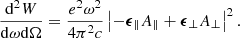 (A.7)
(A.7)
As shown in Figure 1, we consider a charge of identifier of ijk. The vector part of Equation (A.6) can be written as:
![Mathematical equation: $$ \begin{aligned} \begin{aligned}&\boldsymbol{n}\times \left(\boldsymbol{n} \times \boldsymbol{\beta }_{ijk,\Vert }\right)\\&=\beta _\Vert \left[-\boldsymbol{\epsilon }_{\Vert } \sin \left(\frac{v t}{\rho }+\chi _{ij}\right)+\boldsymbol{\epsilon }_{\perp } \cos \left(\frac{v t}{\rho }+\chi _{ij}\right) \sin \varphi _k\right], \end{aligned} \end{aligned} $$](/articles/aa/full_html/2024/05/aa48670-23/aa48670-23-eq88.gif) (A.8)
(A.8)
and the argument of the exponential is:
![Mathematical equation: $$ \begin{aligned} \begin{aligned} \omega \left(t-\frac{\boldsymbol{n} \cdot \boldsymbol{r}_{ijk}(t)}{c}\right)&=\omega \left[t-\frac{2 \rho }{c} \sin \left(\frac{v t}{2 \rho }\right) \cos \left(\frac{v t}{2 \rho }+\chi _{ij}\right) \cos \varphi _k\right]\\&\simeq \frac{\omega }{2}\left[\left(\frac{1}{\gamma ^{2}} +\varphi _k^{2}+\chi _{ij}^{2}\right) t+\frac{c^{2} t^{3}}{3\rho ^{2}}+\frac{c t^{2}}{\rho } \chi _{ij}\right], \end{aligned} \end{aligned} $$](/articles/aa/full_html/2024/05/aa48670-23/aa48670-23-eq89.gif) (A.9)
(A.9)
where t is adopted to replace t′ in the following calculations. Therefore, the two amplitudes for Equation (A.7) are given by:
![Mathematical equation: $$ \begin{aligned} \begin{aligned} A_{ijk,\Vert }&\simeq \int _{-\infty }^{\infty }\left(\frac{c t}{\rho }+\chi _{ij}\right)\\&\times \exp \left(i \frac{\omega }{2}\left[\left(\frac{1}{\gamma ^{2}} +\varphi _k^{2}+\chi _{ij}^{2}\right) t+\frac{c^{2} t^{3}}{3 \rho ^{2}} +\frac{c t^{2}}{\rho } \chi _{ij}\right]\right)\mathrm{d}t, \\ A_{ijk,\perp }&\simeq \varphi _k \int _{-\infty }^{\infty } \exp \left(i \frac{\omega }{2}\left[\left(\frac{1}{\gamma ^{2}} +\varphi _k^{2}+\chi _{ij}^{2}\right) t+\frac{c^{2} t^{3}}{3 \rho ^{2}} +\frac{c t^{2}}{\rho } \chi _{ij}\right]\right)\mathrm{d}t. \end{aligned} \end{aligned} $$](/articles/aa/full_html/2024/05/aa48670-23/aa48670-23-eq90.gif) (A.10)
(A.10)
Making the changes of variables:
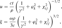 (A.11)
Equation (A.10) becomes:
![Mathematical equation: $$ \begin{aligned} \begin{aligned} A_{ijk,\Vert }&\simeq \frac{\rho }{c}\left(\frac{1}{\gamma ^{2}} +\varphi _{k}^2+\chi _{ij}^2\right)\\&\times \int _{-\infty }^{\infty }\left(u+\frac{\chi _{ij}}{\sqrt{1/\gamma ^{2}+\chi _{ij}^{2}+\varphi _k^2}}\right) \\&\times \exp \left[i \frac{3}{2} \xi \left(u+\frac{1}{3} u^{3}+\frac{\chi _{ij}}{\sqrt{1/\gamma ^{2}+\varphi _k^2+\chi _{ij}^{2}}} u^{2}\right)\right] \mathrm{d} u,\\ A_{ijk,\perp }&\simeq \frac{\rho }{c}\varphi _k\left(\frac{1}{\gamma ^{2}} +\varphi _{k}^2+\chi _{ij}^2\right)^{1/2} \\&\times \int _{-\infty }^{\infty }\exp \left[i \frac{3}{2} \xi \left(u+\frac{1}{3} u^{3}+\frac{\chi _{ij}}{\sqrt{1/\gamma ^{2} +\varphi _k^2+\chi _{ij}^{2}}} u^{2}\right)\right]\mathrm{d} u.\\ \end{aligned} \end{aligned} $$](/articles/aa/full_html/2024/05/aa48670-23/aa48670-23-eq92.gif) (A.12)
(A.12)
We note that:
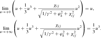 (A.13)
The integrals in Equation (A.12) are identifiable as Airy integrals. Consequently, the two amplitudes are:
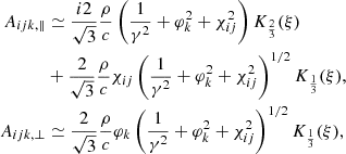 (A.14)
where Kν(ξ) is the modified Bessel function, in which Kν(ξ)→(Γ(ν)/2)(ξ/2)−ν for ξ ≪ 1 and ν ≠ 0, and 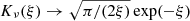 for ξ ≫ 1, leading to a wide-band spectrum.
The curvature radius can be regarded as a constant since the bunch’s size is much smaller than its altitude. We assume that each bunch has roughly the same χu and χd even with different k so that an average height can be derived to replace the complex boundary condition of the bulk (Wang et al. 2022a). Consider that the bunch longitude size is l < 4ρ/(3γ3). The emission with ω < ωc is added coherently. For the emission band with ω > ωl, the emission is added incoherently and the fluxes drop with ω very quickly. The spectrum becomes much deeper than an exponential function. The total amplitudes of a bunch are then given by:
![Mathematical equation: $$ \begin{aligned} \begin{aligned} A_{\Vert }&\simeq \frac{2}{\sqrt{3}}\frac{\rho }{c}\frac{N_j}{\Delta \chi }\frac{N_k}{2\varphi _t}N_i\\&\times \int ^{\chi _{u,i}}_{\chi _{d,i}}d\chi^\prime \int ^{\varphi _u}_{\varphi _d} \left[i\left(\frac{1}{\gamma ^{2}}+\varphi ^{\prime 2}+\chi ^{\prime 2}\right)K_{\frac{2}{3}}(\xi )\right.\\&\left.+\chi^\prime \left(\frac{1}{\gamma ^{2}}+\varphi ^{\prime 2}+\chi ^{\prime 2}\right)^{1/2} K_{\frac{1}{3}}(\xi )\right]\cos \varphi \prime \mathrm{d}\varphi \prime ,\\ A_{\perp }&\simeq \frac{2}{\sqrt{3}}\frac{\rho }{c} \frac{N_j}{\Delta \chi }\frac{N_k}{2\varphi _t}N_i\\&\times \int ^{\chi _{u,i}}_{\chi _{d,i}} d\chi^\prime \int ^{\varphi _u}_{\varphi _d}\left(\frac{1}{\gamma ^{2}} +\varphi ^{\prime 2}+\chi ^{\prime 2}\right)^{1/2}K_{\frac{1}{3}}(\xi ) \varphi \prime \cos \varphi^\prime \mathrm{d}\varphi^\prime , \end{aligned} \end{aligned} $$](/articles/aa/full_html/2024/05/aa48670-23/aa48670-23-eq96.gif) (A.15)
(A.15)
where χu is the upper boundary χ′, χd is the lower boundary χ′, and the boundaries of φ′ read φu = φt + φ and φd = −φt + φ.
With the particular interest of β1, ∥(t) = β1exp(−iωat), the total amplitudes of a bunch for the parallel perturbation are given by:
![Mathematical equation: $$ \begin{aligned} \begin{aligned} \tilde{A}_{\Vert }&\simeq \frac{2}{\sqrt{3}}\frac{\rho }{c}\frac{N_j}{\Delta \chi }\frac{N_k}{2\varphi _t}N_i\beta _1\\&\times \int ^{\chi _{u,i}}_{\chi _{d,i}}d\chi^\prime \int ^{\varphi _u}_{\varphi _d} \left[i\left(\frac{1}{\gamma ^{2}}+\varphi ^{\prime 2}+\chi ^{\prime 2}-\frac{2\omega _a}{\omega }\right) K_{\frac{2}{3}}(\xi _a)\right.\\&\left.+\chi^\prime \left(\frac{1}{\gamma ^{2}}+\varphi ^{\prime 2}+\chi ^{\prime 2} -\frac{2\omega _a}{\omega }\right)^{1/2}K_{\frac{1}{3}}(\xi _a)\right]\cos \varphi^\prime \mathrm{d}\varphi^\prime ,\\ \tilde{A}_{\perp }&\simeq \frac{2}{\sqrt{3}}\frac{\rho }{c}\frac{N_j}{\Delta \chi }\frac{N_k}{2\varphi _t}N_i\beta _1\\&\times \int ^{\chi _{u,i}}_{\chi _{d,i}}d\chi^\prime \int ^{\varphi _u}_{\varphi _d} \left(\frac{1}{\gamma ^{2}}+\varphi ^{\prime 2}+\chi ^{\prime 2}-\frac{2\omega _a}{\omega }\right)^{1/2}\\&\times K_{\frac{1}{3}}(\xi _a)\varphi^\prime \cos \varphi^\prime \mathrm{d}\varphi^\prime . \end{aligned} \end{aligned} $$](/articles/aa/full_html/2024/05/aa48670-23/aa48670-23-eq97.gif) (A.16)
(A.16)
The monochromatic perturbation frequency is Doppler boosted to 2γ2ωa, so that there is a spike in the spectrum at ω = 2γ2ωa, and the width of the spike is determined by the boundaries of χ′ and φ′.
We consider the case with a similar formula but for the perpendicular perturbation, namely, β1, ⊥(t) = β1exp(−iωat). Following the discussion in Section 2.2.4, we insert Equation (12) into Equation (15) and the amplitudes are calculated as:
![Mathematical equation: $$ \begin{aligned} \begin{aligned} \tilde{A}_{ijk,\Vert }&\simeq \frac{1}{\sqrt{3}}\frac{\rho }{c}\beta _1 (\varphi _k^2-\chi _{ij}^2)\left(\frac{1}{\gamma ^{2}}+\varphi ^{\prime 2} +\chi ^{\prime 2}-\frac{2\omega _a}{\omega }\right)^{1/2}K_{\frac{1}{3}}(\xi _a)\\&-\frac{i2}{\sqrt{3}}\frac{\rho }{c}\beta _1\chi _{ij}\left(\frac{1}{\gamma ^{2}} +\varphi ^{\prime 2}+\chi ^{\prime 2}-\frac{2\omega _a}{\omega }\right)K_{\frac{2}{3}}(\xi _a)\\&+\frac{\rho }{c}\beta _1\left(\frac{1}{\gamma ^{2}}+\varphi ^{\prime 2} +\chi ^{\prime 2}-\frac{2\omega _a}{\omega }\right)^{3/2}\\&\times \left[\frac{1}{\sqrt{3}}K_{\frac{1}{3}}(\xi _a)-\pi \delta \left(3\xi _a/2\right)\right],\\ \tilde{A}_{ijk,\perp }&\simeq -\frac{i2}{\sqrt{3}}\frac{\rho }{c}\varphi _k\beta _1 \left(\frac{1}{\gamma ^{2}}+\varphi _{k}^2+\chi _{ij}^2\right)K_{\frac{2}{3}}(\xi _a)\\&-\frac{2}{\sqrt{3}}\frac{\rho }{c}\varphi _k\beta _1\chi _{ij} \left(\frac{1}{\gamma ^{2}}+\varphi _{k}^2+\chi _{ij}^2\right)^{1/2}K_{\frac{1}{3}}(\xi _a),\\ \end{aligned} \end{aligned} $$](/articles/aa/full_html/2024/05/aa48670-23/aa48670-23-eq98.gif) (A.17)
(A.17)
where δ(x) is the Dirac function. The total amplitudes of a bunch for the perpendicular perturbation case can be given by the integrals of Equation (A.17).
Appendix B: Stokes parameters
Four Stokes parameters are significant tools to describe the polarization properties of a quasi-monochromatic electromagnetic wave. In this section, we consider the monochrome Stokes parameters which can be derived by the Fourier-transformed electric vector. The Fourier-transformed polarized components of electric waves can be written as:
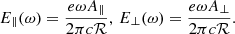 (B.1)
(B.1)
By inserting Equation (B.1), four Stokes parameters of observed waves can be calculated as:
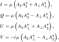 (B.2)
(B.2)
where μ = ω2e2/(4π2ℛ2c𝒯) is the proportionality factor, I defines the total intensity, Q and U define the linear polarization and its position angle, and V describes circular polarization. The timescale 𝒯 is chosen as the average timescale the flux density I repeated. The corresponding linear polarization and PA are then given by:
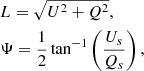 (B.3)
(B.3)
where
 (B.4)
(B.4)
where ψ is given by the rotation vector model (RVM; Radhakrishnan & Cooke 1969).
Appendix C: Quake-induced oscillation
We calculated the frequencies of the torsional modes for the relativistic star caused by a quake and discuss the effect of the magnetic field on the frequencies of the various torsional modes. Oscillations after the quake have two types: spherical and toroidal, in which only the toroidal oscillations can effectively modify the spin of the star and the Goldreich-Julian density. The axial perturbation equations for the elastic solid star in the Cowling approximation is written as (Samuelsson & Andersson 2007; Sotani et al. 2012):
![Mathematical equation: $$ \begin{aligned} \begin{aligned}&Y\left[\frac{\rho _m+P}{\mu }\,\Omega ^2 \exp (-2\Phi )-\frac{(\ell +2)(\ell -1)}{r^2}\right]\exp ({2\Lambda }) + Y^{\prime \prime }\\&+\left(\frac{4}{r}+\Phi^\prime -\Lambda^\prime +\frac{\mu^\prime }{\mu }\right) Y^\prime = 0, \end{aligned} \end{aligned} $$](/articles/aa/full_html/2024/05/aa48670-23/aa48670-23-eq103.gif) (C.1)
(C.1)
where μ is the shear modulus, Φ and Λ are functions of r, ρm is the mass-energy density, Y(r) describes the radial part of the angular oscillation amplitude, and the integer ℓ is the angular separation constant which enters when Y(r) is expanded in spherical harmonics Yℓm(θ, ϕ).
To discuss the possible effects of the magnetic field, we extended our study to the torsional oscillation of a magnetized relativistic star (e.g., Li et al. 2024). Sotani et al. (2007) derived the perturbation equations of the magnetized relativistic star using the relativistic Cowling approximation. The final perturbation equation is:
 (C.2)
(C.2)
where the coefficients are given in terms of the functions describing the equilibrium metric, fluid, and the magnetic field of the star:
 (C.3)
(C.3)
![Mathematical equation: $$ \begin{aligned} B_{\ell }(r)&=\left(\frac{4}{r} + \Phi^\prime - \Lambda^\prime \right)\mu + \mu^\prime \nonumber \\&+ (1 + 2\lambda _1)\frac{a_1}{\pi r^4}\left[\left(\Phi^\prime - \Lambda^\prime \right)a_1 + 2{a_1}\prime \right] , \end{aligned} $$](/articles/aa/full_html/2024/05/aa48670-23/aa48670-23-eq106.gif) (C.4)
(C.4)
![Mathematical equation: $$ \begin{aligned} C_{\ell }(r)&= (2 + 5\lambda _1)\frac{a_1}{2\pi r^4}\left\{ \left(\Phi^\prime - \Lambda^\prime \right){a_1}^\prime + {a_1}^{\prime \prime }\right\} \nonumber \\&- (\lambda -2)\left(\frac{ \mu \exp (2\Lambda )}{r^2} - \frac{\lambda _1{{a_1}^\prime }^2}{2\pi r^4}\right) \nonumber \\&+\left[\left(\rho _m + P + (1 +2\lambda _1)\frac{{a_1}^2}{\pi r^4} \right)\exp (2\Lambda ) - \frac{\lambda _1 {{a_1}^\prime }^2}{2\pi r^2}\right]\\&\times \Omega ^2 \exp (-2\Phi ) \nonumber , \end{aligned} $$](/articles/aa/full_html/2024/05/aa48670-23/aa48670-23-eq107.gif) (C.5)
(C.5)
where λ = ℓ(ℓ + 1), and λ1 = −ℓ(ℓ+1)/[(2ℓ−1)(2ℓ+3)]. To solve Eqs. (C.1) and (C.2) and determine the oscillation frequencies, the boundary conditions require that the traction vanishes at the top and the bottom of the crust.
The toroidal oscillations can effectively modify the spin and the electric field in the gap. The velocity components of toroidal oscillations can be written as:
![Mathematical equation: $$ \begin{aligned} \delta v^{\hat{i}}=\left[0, \frac{1}{\sin \theta } \partial _\phi Y_{\ell m}(\theta , \phi ),-\partial _\theta Y_{\ell m}(\theta , \phi )\right] \tilde{\eta }(r) e^{-i \Omega t}, \end{aligned} $$](/articles/aa/full_html/2024/05/aa48670-23/aa48670-23-eq108.gif) (C.6)
(C.6)
where  is a parameter denoting the amplitude of the oscillations. Owing to unipolar induction, we have (Lin et al. 2015):
![Mathematical equation: $$ \begin{aligned} E_\theta = -\frac{1}{N c}\left[\frac{2\pi r}{P} \sin \theta \left(1-\frac{R^3\kappa }{r^3}\right)-\partial _\theta Y_{\ell m} \tilde{\eta }(r)\right] B_{\rm s} \frac{f(r)}{f(R)} \frac{R^3\cos \theta }{r^3}, \end{aligned} $$](/articles/aa/full_html/2024/05/aa48670-23/aa48670-23-eq110.gif) (C.7)
(C.7)
where  , κ = 2GIm/(R3c2), Im is the moment of inertia, and f(r) is:
![Mathematical equation: $$ \begin{aligned} f(r)=-3\left(\frac{rc^2}{2GM}\right)^3\left[\ln \left(1-\frac{2GM}{rc^2}\right)+\frac{2GM}{rc^2}\left(1+\frac{GM}{ rc^2}\right)\right]. \end{aligned} $$](/articles/aa/full_html/2024/05/aa48670-23/aa48670-23-eq112.gif) (C.8)
(C.8)
Appendix D: Dispersion relationship of ultra-relativistic plasma
In this section, we briefly summarize the physics of waves in ultra-relativistic plasma. Basically, the equation of motion of a given charge species is expressed as:
 (D.1)
(D.1)
where vs = vs, 0 + δvs, E = δE, B = B0 + δB, in which δvs, δE, δB are associated with the disturbance in the plasma and have a form of exp[ − i(ωt − k ⋅ r)]. Combined with
 (D.2)
(D.2)
and
 (D.3)
(D.3)
δvs can be then described in terms of δE. The continuity equation is expressed as:
 (D.4)
(D.4)
so that the density perturbation is given by:
 (D.5)
(D.5)
The conductivity tensor σ is defined by:
 (D.6)
(D.6)
and the dielectric tensor is given by:
 (D.7)
(D.7)
where I is the unit tensor. Since the electric displacement vector is defined as D = ϵ ⋅ E, we can obtain the equation for plane waves in a coordinate system (x′, y′, z′) where B0 goes along z′ as follows:
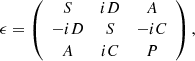 (D.8)
(D.8)
with
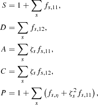 (D.9)
(D.9)
where
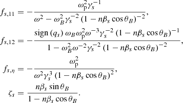 (D.10)
Here, the subscript ‘0’ has been suppressed. In the coordinate system x0y0z0 with k along the z0-axis and B in the x0 − z0 plane, the components of dielectric tensor are given by:
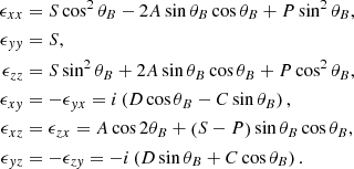 (D.11)
The three electric components have:
 (D.12)
Reinserting this back into the definition of electric displacement vector yields:
 (D.13)
where
![Mathematical equation: $$ \begin{aligned} \begin{aligned} \eta _{x x}&=\frac{1}{\epsilon _{z z}}\left(\epsilon _{z z} \epsilon _{x x}-\epsilon _{x z} \epsilon _{z x}\right) =\frac{1}{\epsilon _{z z}}\left(SP -A^2\right), \\ \eta _{y y}&=\frac{1}{\epsilon _{z z}}\left(\epsilon _{z z} \epsilon _{y y}-\epsilon _{y z} \epsilon _{z y}\right), \\&=\frac{1}{\epsilon _{z z}}\left[\left(S^{2}-D^2-S P +C^2\right) \sin ^2 \theta _B\right]\\&+\frac{1}{\epsilon _{z z}}\left[2\left(A S -C D\right) \sin \theta _B \cos \theta _B+S P -C^2\right] \\ \eta _{y x}&=-\eta _{x y}=\frac{1}{\epsilon _{z z}} \left(\epsilon _{z z} \epsilon _{y x}-\epsilon _{y z}\epsilon _{z x}\right), \\&=\frac{-i}{\epsilon _{z z}}\left[PD \cos \theta _B-S C \sin \theta _B+A\left(D \sin \theta _B-C \cos \theta _B\right)\right]. \end{aligned} \end{aligned} $$](/articles/aa/full_html/2024/05/aa48670-23/aa48670-23-eq126.gif) (D.14)
(D.14)
For a normal pulsar or magnetar, one can obtain ωB ≫ ω and ωB ≫ ωp inside the magnetosphere. Under these conditions, some parameters can be reduced to:
 (D.15)
Reinserting this back into Equation (D.13) and the solution of refractive index is given by (Arons & Barnard 1986):
![Mathematical equation: $$ \begin{aligned} \begin{aligned}&n^2=1,\\&n^2=\eta _{xx},\\&\left(\omega ^2-c^2 k_{\Vert }^2\right)\left[1-\frac{\omega _{\mathrm{p},s}^2}{\gamma _s^3\omega ^2(1-\beta _s c k_{\Vert }/\omega )}\right]-c^2 k_{\perp }^2=0, \end{aligned} \end{aligned} $$](/articles/aa/full_html/2024/05/aa48670-23/aa48670-23-eq128.gif) (D.16)
(D.16)
where k∥ = kcosθB and k⊥ = ksinθB. For the mode with n2 = 1, the polarization is given by:
 (D.17)
As a result, the mode is a transverse wave with the electric field vector in the k × B direction, that is, the X-mode. For the other two refractive index solutions, we can obtain:
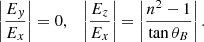 (D.18)
The mode is called O-mode which the electric field oscillates at k − B plane.
We plot the dispersion relationship of the X-mode and the O-mode for two cases (γ = 2 and γ = 10) in Figure D.1. For both cases, θB = 0.2 is adopted. The O-modes have two branches: the superluminous branch (n < 1) and the subluminous branch (n > 1). The superluminous O-mode has a frequency cut-off at ωγ3 = ωp. The latter one has a refractive index cut-off at n = 1/cosθB. This mode looks to have two branches as shown in Figure D.1, but the branches can get crossed at high frequencies.
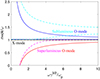 |
Fig. D.1. Refractive indices of wave modes as a function of ωγ3/ωp with θB = 0.2 for two cases: γ = 2 (dashed lines) and γ = 100 (solid lines). The black dotted-dashed line shows the X-mode (n = 1). The O-modes have two branches: subluminous O-mode (cyan dashed line for γ = 2 and blue solid line for γ = 10) and superluminous O-mode (magenta dashed line for γ = 2 and red solid line for γ = 10). |
Appendix E: Notation List
Subscript i, j, k: The identifier of each charged particle
Subscript s: Species of a single particle c: Speed of light
d2W/dωdΩ: Energy radiated per unit solid angle per unit frequency interval
e: Charge (absolute value) of electron
f(u): Distribution function of plasma
hgap: Height of the gap
k: Wave vector
kB: Boltzmann constant
l: Longitude bunch size
ℓ: Angular separation constant
me: Mass of the electron
n: Unit vector of the line of sight
n: Refractive index
ne: Number density of charges
nGJ: Goldreich-Julian density
np: Number density of magnetospheric plasma
p: Power law index
r: Distance to the neutron star center
s: Distance that charges traveled along the field lines
u: Space-like part of the four-velocity
um: Average u over the Gaussian distribution
v: Velocity of electron
w: Burst width
A∥: Parallel component of amplitude
A⊥: Perpendicular component of amplitude
B: Magnetic field strength
E: Wave electric field
E1, ∥: Perturbation electric field parallel to the B-field
E1, ⊥: Perturbation electric field perpendicular to the B-field
E∥: Electric field parallel to the B-field
I, Q, U, V: Stokes parameters
J: Current density
j: Emissivity
Kν: Modified Bessel function
ℒb: Luminosity of a bunch
M: Stellar mass
ℳ: Multiplicity factor
Nb: Number of bunches that contribute to the observed power at an epoch
Ne: Number of electrons in one bunch
Ni: Maximum number of the subscript of i
Nj: Maximum number of the subscript of j
Nk: Maximum number of the subscript of k
P: Spin period
R: Stellar radius
Rb: Transverse size of bunch
ℛ: Distance from the emitting source to the observer
T: Temperature
𝒯: The average timescale of the flux density I repeated
Yℓm(θ, ϕ): Spherical harmonics
α: Angle between spin axis and magnetic axis
β: Dimensionless velocity of one charge
 : Dimensionless perturbation acceleration parallel to the B-field
 : Dimensionless perturbation acceleration perpendicular to the B-field
δV: Vacuum polarization coefficient
γ: Lorentz factor
μ: Shear modulus ν: Frequency, index of the modified Bessel function
 : Drift rate
χ: Angle between  for different trajectories
χd: Lower boundary of angle between  for different trajectories
χu: Upper boundary of angle between  for different trajectories
ϵ: Dielectric tensor
λ: Wavelength
ψ: Polarization angle given by the RVM model
ρ: Curvature radius
σ: Conductivity tensor
σc: Curvature cross section
τ: Optical depth
θ: Poloidal angle with respect to the magnetic axis
θc: Spread angle of the curvature radiation
θin: Angle between the incident photon momentum and the electron momentum
θs: Angle of the footpoint for field line at the surface
θB: Angle between angle between  and
and 
ω: Angular frequency
ωa: Frequency of the perturbation-induced acceleration
ωB: Cyclotron frequency
ωc: Critical frequency of curvature radiation
ωcut: Angular frequency cut-off of the superluminous O-mode
ωin: Angular frequency of incoming wave of ICS
ωM: Frequency of bulk of bunches distribution
ωp: Plasma frequency
φ: Azimuth angle to the magnetic axis, the angle between LOS and the trajectory plane
φd: Lower boundary of angle between LOS and the trajectory plane
φt: Half opening angle of a bulk of bunches
φu: Upper boundary of angle between LOS and the trajectory plane
Γ(ν): Gamma function
Ψ: Polarization angle
Θe: Magnetic colatitude of the emission point
Ω: Solid angle of radiation, angular frequency of the oscillations.
All Figures
|
Fig. 1. Schematic diagram of a bulk of bunches moving in the magnetosphere is shown in the left panel. The light solid blue line shows the slice in which electrons emit roughly the same phase. The unit vector of the LOS is denoted as n, while ϵ1 and ϵ2 denote the two polarization components. The geometry for instantaneous circular motion for a particle identified by ijk in a bunch is on the right. The trajectory lies on the β0, ∥ − ϵ1 plane. At the retarded time, t = 0, the electron is at the origin. The dotted trajectory shows an electron at the origin. The angle between the solid and dotted trajectory is χij at t = 0. The angle between the LOS (z0) and the trajectory plane is φk. |
| In the text | |
|
Fig. 2. Normalized spectra of the quasi-periodically structured bulk of bunches: (a) ωM = 108 Hz; (b) ωM = 5 × 10⁸ Hz. The black solid line is the spectrum due to the quasi-periodic structure. The blue dashed line is the spectrum of a uniformly distributed bulk of bunches. |
| In the text | |
|
Fig. 3. Normalized spectra of the parallel perturbation cases at φ = 0: φt = 0.1/γ, β1 = 10−6 (blue dashed line); φt = 0.1/γ, β1 = 10−5 (red dotted line); φt = 1/γ, β1 = 10−6 (black solid line); and φt = 1/γ, β1 = 10−5 (green dashed-dotted line). |
| In the text | |
|
Fig. 4. Normalized spectra of the perpendicular perturbation cases at φ = 0: φt = 0.1/γ, β1 = 10−4 (blue dashed line); φt = 0.1/γ, β1 = 10−3 (red dotted line); φt = 1/γ, β1 = 10−4 (black solid line); and φt = 1/γ, β1 = 10−3 (green dashed-dotted line). |
| In the text | |
|
Fig. 5. Simulated polarization profiles for the bunch with γ = 102, φt = 10−2, ρ = 107 cm. Top panel: polarization position angle envelope. Middle panel: total polarization fraction (black solid line), linear polarization fraction (red dashed line), and circular polarization fraction (blue dashed-dotted line). Bottom: total intensity, I, (black solid line), linear polarization, L, (red dashed line), and circular polarization, V, (blue dashed-dotted line) as functions of φ. All three functions are normalized to the value of I at φ = 0. |
| In the text | |
|
Fig. 6. Frequencies of the second overtone n = 2 and ℓ = 2 torsional modes as a function of the normalized magnetic field (B/Bμ). The NS mass is M = 1.4 M⊙. The dashed lines correspond to our fits using the empirical formula (21) with different coefficient values. The fitting values are 2.4, 0.78, 2.2, and 0.69 for WFF3+ DH model, WFF3+ NV model, A+ DH model, and A+ NV model, respectively. |
| In the text | |
|
Fig. 7. Optical depths for four distributions: Jüttner with ρT = 0.1 (black solid line), Gaussian with |
| In the text | |
|
Fig. 8. Normalized spectra of self-absorbed curvature radiation. Black lines denote purely bunching curvature radiations for φt = 0.1/γ (solid line) and φt = 1/γ (dashed-dotted line). Blue lines denote the radiation after curvature self-absorption for φt = 0.1/γ (solid line) and φt = 1/γ (dashed-dotted line). |
| In the text | |
|
Fig. 9. Comparison of drift rates at different frequencies. Different regions show the 1σ region of the best fitting results: FRB 20121102A (blue), FRB 180916B(red), and all FRBs (grey). |
| In the text | |
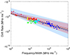 |
Fig. 10. Same as Fig. 9 but for comparison of drift rates at different frequency and width. |
| In the text | |
|
Fig. D.1. Refractive indices of wave modes as a function of ωγ3/ωp with θB = 0.2 for two cases: γ = 2 (dashed lines) and γ = 100 (solid lines). The black dotted-dashed line shows the X-mode (n = 1). The O-modes have two branches: subluminous O-mode (cyan dashed line for γ = 2 and blue solid line for γ = 10) and superluminous O-mode (magenta dashed line for γ = 2 and red solid line for γ = 10). |
| In the text | |
Current usage metrics show cumulative count of Article Views (full-text article views including HTML views, PDF and ePub downloads, according to the available data) and Abstracts Views on Vision4Press platform.
Data correspond to usage on the plateform after 2015. The current usage metrics is available 48-96 hours after online publication and is updated daily on week days.
Initial download of the metrics may take a while.