| Issue |
A&A
Volume 696, April 2025
|
|
|---|---|---|
| Article Number | A187 | |
| Number of page(s) | 11 | |
| Section | The Sun and the Heliosphere | |
| DOI | https://doi.org/10.1051/0004-6361/202553752 | |
| Published online | 18 April 2025 | |
Dynamic spectra of solar radio emissions from weak-turbulence simulation
1
Centre for Mathematical Plasma Astrophysics, Department of Mathematics, KU Leuven, Celestijnenlaan 200B, B-3001 Leuven, Belgium
2
Institute for Theoretical Physics IV, Faculty for Physics and Astronomy, Ruhr University Bochum, D-44780 Bochum, Germany
3
Instituto de Física, Universidade Federal do Rio Grande do Sul, 91501-970 Porto Alegre, RS, Brazil
4
Institute for Physical Science and Technology, University of Maryland, College Park, MD 20742-2431, USA
5
Research Center in the intersection of Plasma Physics, Matter, and Complexity ( P 2 mc), Comisión Chilena de Energía Nuclear, Casilla 188-D, Santiago, Chile
6
Departamento de Ciencias Físicas, Facultad de Ciencias Exactas, Universidad Andres Bello, Sazié 2212, Santiago 8370136, Chile
7
Institute of Physics, University of Maria Curie-Sklodowska, ul. Radziszewskiego 10, 20-031 Lublin, Poland
⋆ Corresponding author; This email address is being protected from spambots. You need JavaScript enabled to view it.
Received:
14
January
2025
Accepted:
8
March
2025
Abstract
Context. In recent decades, serious efforts have been made in the analytical and numerical modeling of solar radio bursts generated by the electron beam interacting with the background plasma, including the dynamic spectra with decreasing frequency over time/space. These are type II and type III radio bursts, with the fundamental components at the local plasma frequency (ωp = 2πfp) and the harmonics (nωp = 2πnfp). Synthetic spectra built for a number of radio events were able to reproduce the decreasing frequency profiles reasonably well, despite the limitations of the approximate analytical theory.
Aims. We propose new modeling of dynamic radio emission spectra using weak-turbulence (WT) theory. This novel approach also aims at a self-consistent and quantitative evaluation of radio emissions, based on first-principles modeling of electron beam plasma instabilities and nonlinear wave interaction.
Methods. We performed the WT simulation, which has the ability to quantitatively describe the standard plasma emission involving the nonlinear interaction of Langmuir (L), ion-sound (S), and transverse electromagnetic (T) waves. The composite dynamic spectra are constructed for type II- and type III-like events, against the background electron density model that behaves as an inverse square of the distance from the solar source.
Results. The new dynamic spectra are obtained distinctly, with a rapid frequency shift for type III emissions (generated by fast electron beams from coronal sources), as well as a less steep frequency drop for type II spectra (whose sources move away from the Sun along with interplanetary shocks). Upon making a qualitative comparison with typical solar radio emission events, we find that our first-principle-based synthetic dynamic spectra are in good agreement.
Conclusions. The findings of the present study demonstrate that the theoretical approach taken in this paper can be further applied to obtain (i) quantitatively relevant predictions and replications of the observed dynamic spectra of radio bursts, and (ii) more realistic large-scale models of the solar radio source, for example the type II and type III source models computed from the large-scale magnetohydrodynamics (MHD) simulations or even from direct spacecraft observations.
Key words: Sun: corona / Sun: coronal mass ejections (CMEs) / Sun: flares / Sun: radio radiation
© The Authors 2025
 Open Access article, published by EDP Sciences, under the terms of the Creative Commons Attribution License (https://creativecommons.org/licenses/by/4.0), which permits unrestricted use, distribution, and reproduction in any medium, provided the original work is properly cited.
This article is published in open access under the Subscribe to Open model. This email address is being protected from spambots. You need JavaScript enabled to view it. to support open access publication.
1. Introduction
The current efforts to understand the physical processes at the origin of radio emissions, mainly plasma emission mechanisms (Henri et al. 2019; Sauer et al. 2019; Lee et al. 2019, 2022; Lazar et al. 2023; Bacchini & Philippov 2024), are a response to a major interest in exploiting them in various applications in astronomy, astrophysics, and solar physics. Of particular importance are solar radio bursts alerting us about energetic solar and space weather events, such as coronal flares, solar energetic particles (SEPs), and coronal mass ejections (CMEs) (Richardson et al. 2018; Kumari et al. 2023; Nedal et al. 2023; Ndacyayisenga et al. 2025). Because space missions can often reveal their unique counterparts in situ (Ergun et al. 1998; Bale et al. 1999; Pulupa & Bale 2008; Pulupa et al. 2010; Manini et al. 2023), which should facilitate the construction of realistic radiative models.
Dynamic spectra showing a decreasing frequency over time and space are characteristic of type II and type III radio bursts triggered by solar events (McLean & Labrum 1985; Ergun et al. 1998; Bale et al. 1999; Schmidt et al. 2013; Hegedus et al. 2021). In both cases, the standard plasma emission model that results from the partial conversion of electrostatic waves to the radiation energy applies (Melrose 2008). The electrostatic wave energy is first generated by the interaction of the electron beam and the background plasma via what is known as the bump-in-tail instability, which leads to Langmuir (L) wave excitations at local plasma frequency ωp = 2πfp (Sagdeev & Galeev 1969; Davidson 1972). At sufficiently high intensities L-waves can undergo nonlinear wave-wave decays or couplings (e.g., with low-frequency ion sound (S) waves), as well as nonlinear wave-particle interaction with the background thermal ions, and can ultimately generate transverse (T) radio waves (Melrose 1980; Ziebell et al. 2015). In association with type II emissions, single or double (counter-propagating) electron beams are observed, and are supposed to be accelerated and reflected by the interplanetary (IP) CME shock (Roberts 1959; Cairns et al. 2003; Gopalswamy et al. 2005). The energy-releasing processes at the coronal flares generate energetic electron beams that propagate along the open magnetic field lines and produce type III emissions (Lin et al. 1981; Ergun et al. 1998; Reid & Ratcliffe 2014) and impulsive solar energetic particle (SEP) events (Reames 2021). In addition, the CME is associated with energetic protons and the gradual SEP events (Reames 2021), which are energetically more important than electrons, and thus the detection of type II emissions has significant implications for the space weather forecast perspective (Cairns et al. 2003).
These radio bursts exhibit a decreasing frequency feature, which is evidence that they excite radio emission at local plasma frequency as they move away from the Sun. As these radio bursts extend to many decades in frequency, it is clear that their sources traverse sufficiently large distances in the IP space. The difference between the two types of radio bursts is quite apparent: type II emissions have a drift of decreasing frequency imprinted by the bulk speed of the CME front, resulting in a much more gradual drift in frequency than the abrupt downward drift of type III emissions (see Fig. 1, which illustrates this). Other examples of dynamic spectra observed for type II and type III radio emissions are shown in Fig. 1 in the paper by Schmidt et al. (2013). The much faster drift and much higher intensity of type III solar bursts are signatures of the very energetic electron beams at their origin. Since the plasma density falls off as roughly 1/r2 in the solar wind, where r is the (radial) distance from the surface of the Sun, the plasma frequency and the observed frequency drift down as 1/r.
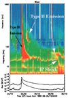 |
Fig. 1. Dynamic spectra from the WAVES experiment on Wind (upper panels) and GOES-10 soft X-ray flux data (bottom panel). A flare at 22:09:11 UT on August 24, 1998, is associated with an abrupt onset of soft X-ray flux and the intense type III burst, while the type II burst has a slow frequency-drifting feature, preceding the IP shock generated by the CME. After Bale et al. (1999). |
The progress recorded in the last decades by the observational interpretation of dynamic radio spectra should be noted, especially in revealing the spatial and temporal features of their sources. Thus, the observed dynamic spectra of type II radio emissions have been used in combination with white light coronagraph data (Mäkelä et al. 2016), and also with macro-simulations of CME expansion (Magdalenic et al. 2014) to identify the source direction and even its position at the front of IP shock. The tracking of the source of type II radio emissions was also done by comparing the observations with the source models and synthetic dynamic spectra produced with analytical kinetic models and magnetohydrodynamics (MHD) models (Schmidt et al. 2013; Schmidt & Cairns 2016; Hegedus et al. 2021). For the characterization of type III radio sources, observational techniques were proposed to compare the dynamic spectra measured, for instance, by different instruments in space (e.g., STEREO A, B, and Wind; Thejappa et al. 2012) or even those measured on the ground by LOFAR with those detected by the Parker Solar Probe (PSP) at low heliocentric distances (Nedal et al. 2023).
In this paper, we present dynamic spectra predicted for the first time by weak-turbulence theory (WT), for both type II and type III solar radio bursts. The WT theory proves to be a valuable approach for investigating and modeling kinetic plasma processes (Yoon 2019), both linear and quasilinear (QL), but also nonlinear phenomena responsible for plasma radio emission (Ziebell et al. 2014, 2015, 2016; Lee et al. 2019; Ziebell 2021). Compared to numerical simulations (Henri et al. 2019; Sauer et al. 2019; Lazar et al. 2023), this semi-analytical method involves much faster numerical solvers and far fewer computational resources, but contributes significantly to the physical understanding of simulations (Lee et al. 2019). It has been applied for various parameterizations and configurations of electron beams, specific to type II and type III emission sources, induced by unidirectional and bidirectional beams of electrons (Ziebell et al. 2014, 2015, 2016; Ziebell 2021). Counterbeams or bidirectional beams are associated with IP shocks and closed magnetic topologies.
The present paper is structured as follows. Section 2 begins with a brief review of the models of (synthetic) dynamic spectra proposed to date. We then provide a straightforward physical formalism that can directly explain the temporal and spatial descending profiles of the dynamic frequency spectra from the observations of solar radio bursts. The methodology used to build the new dynamic spectra is described in detail in Sect. 3. The synthetic spectra are elaborated for both type II and type III emissions, as iterations at successive time steps of the local spectra computed self-consistently with the WT approach. One can thus extend the results of a local WT simulation, as temporal and spatial simulations of radio emissions, and seek extended quantitative replication and prediction of the observed spectra by capturing not only the frequency, but also the intensity variations. In Sect. 4 we draw our main conclusions and discuss some perspectives opened by the present results.
2. Synthetic dynamic spectra
Dynamic radio spectra were modeled for type II radio emissions associated with the foreshock caused by coronal plasma ejections (CMEs) (Schmidt & Cairns 2012a,b, 2014), as well as type III solar radio bursts linked to coronal flares and energetic electrons propagating in IP space (Li & Cairns 2013a, 2014). Similar, yet different methods were used for each type of radio burst.
First, we recall the analytical constructions of type II spectra from the radiative formalism of Schmidt and Cairns. It treats multiple physical processes, from shock electron acceleration, to the formation and reflection of electron beams (with Kappa velocity distributions), the excitation of Langmuir waves and their conversion to electromagnetic (EM) radiation (Schmidt & Cairns 2012a). This extended analytical model was then used to construct synthetic radio sources and synthetic dynamic spectra (Schmidt & Cairns 2012b), which were further applied in MHD numerical simulations of IP shocks driven by CMEs (Schmidt et al. 2013; Schmidt & Cairns 2014). Comparisons with the intermittent but long-lasting spectra observed by the STEREO A/B spacecraft prove even the ability of these simulations with synthetic radio sources to provide quantitative predictions for the dynamic type II radio spectra (Schmidt & Cairns 2016). Synthetic spectra were computed as volume emissivities throughout the upstream region for each emission in part, the fundamental (F) at fp, and the second harmonic (H) at 2fp (Schmidt & Cairns 2012a,b). Only approximate, otherwise well-documented analytical expressions were invoked for the properties of the electron beams and their wave excitations, as well as the energy conversion to primary Langmuir excitations and also to secondary waves, including radio emissions triggered by nonlinear wave-wave couplings or decays. These are evaluated with a stochastic growth theory in the limit of marginal stability but dealing with stochastic fluctuations due to variations in the beam and background plasma. The electron beam trajectories are followed into the upstream region of the shock starting from the shock front, and the volume emissivities are mapped along these paths. The flux density of radiation is obtained by integrating over the source volume and does not account for the refraction, absorption, and angular or spatial diffusion effects for propagation in IP medium. Summations are repeated at successive time steps during the simulation to produce time-dependent dynamic spectra. The reduction in time and space of the plasma density and, implicitly, of the radio frequency is given by the radial velocity of the CME, which can be estimated from observations or simulations. For example, the ascension of the coronal loop modeled by Schmidt et al. (2013) provides approximately the same bulk velocity as the chosen CME event.
Regarding type III radio bursts, notable is the long series of works by Li, Cairns, and collaborators, of which here we only comment on those dedicated to the modeling of dynamic spectra (Li et al. 2008a,b; Li & Cairns 2013a,b, 2014). Their models compute the dynamic spectra of both radio emissions, (either for F or for both F and second-H emissions) (e.g., the radio flux Φ(t, f), as a function of time (t) and frequency (f)) and aimed to predict measurements by a remote observer, for example at 1 AU. The radio flux is calculated using approximate analytical models, which account for (1) 1D or even 3D dynamics of electron beams in the plasma source, (2) properties of electron beam plasma instabilities and QL wave-particle interactions, (3) nonlinear wave-wave interactions of Langmuir and ion-sound and generation of EM waves at the fundamental (fp) and second harmonic (2fp) of the plasma frequency, and (4) propagation of EM radiation from the corona to IP space.
The downward frequency drifts associated with the radio bursts are due to the beam propagation into regions of lower density. In the plasma emission scenario, the variation of the solar wind density with the heliocentric distance can be derived from the speed of type III electron beam and the frequency drift rate of type III bursts. Equivalently, for a given density model, a quantitative relation exists between the frequency drift rate and beam speed. The simplest relation can be written as (Wild 1950)
 (1)
(1)
To arrive at Eq. (1) in the QL simulations the following assumptions are made: (i) the beam moves radially at an average, constant speed Vb, (ii) the radiation is produced at f = fp(r) or f = 2fp(r), (iii) rays propagate at constant speed (i.e., c) from the source to the observer, (iv) propagation effects (e.g., refraction and scattering) are negligible, and (v) the time difference for peak radio emission at any two locations is same as the time difference for the arrival of beam at these locations (Li et al. 2008a,b). Various dynamic models can be derived by switching on or off the terms corresponding to these assumptions/effects.
The time variation of the frequency f, which is associated to the local plasma frequency ωp = 2πf = (4πne2/me)1/2 can be obtained from Eq. (1) by assuming n(r) = α/r2 (Richardson 2010; Adhikari et al. 2014; Vocks et al. 2018), 1 leading to
 (2)
(2)
where dr/dt = Vb for type III emissions, or dr/dt = VCME for type II bursts. Thus, for type III emissions, one finds
 (3)
(3)
since r(t) = Vb(t − t0)+r0, where r0(t0) are the coordinates of the initial frequency measurements. Finally
 (4)
(4)
where we can consider, as reference, rE = 1 AU and fE = f(rE) at Earth, whose values are known. For example, for nE ≃ 10 cm−3 we find fE ≃ 180 kHz ≃0.2 MHz, and at t0 we have f(t0) = f0 = C0/r0, implying C0 = f0r0 = fErE.
A similar expression can be obtained for the frequency of type II emissions, and to take into account the CME-imposed motion of their plasma sources, we replace Vb with VCME in Eq. (4) to obtain
 (5)
(5)
An even more general expression can be derived from Eq. (4),
 (6)
(6)
in terms of the time τE = rE/Vb needed for the electron beam to travel the Sun-Earth distance (rE), and the initial/reference position η = r0/rE < 1 in units of rE = 1 AU.
Semiquantitative agreements can be obtained, for example, with the events in Fig. 1, reproduced from Bale et al. (1999), or those analyzed by Schmidt et al. (2013) – see, specifically, their Fig. 1. Here in Fig. 2 we use Eqs. (4) and (5) to roughly reproduce the frequency profiles of the observed solar radio bursts, downshifting with time and implicitly with distance. Type II dynamic spectrum is given by
 (7)
(7)
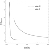 |
Fig. 2. Frequency downshift from Eqs. (2)–(4) for type III and type II spectra, with, respectively, the following parameters: τE = 42 and 840 min, t0 = 115 and 135 min, and η = 0.02 and 0.035. There is agreement of these profiles with the spectra in Fig. 1, and Fig. 1 in Schmidt et al. (2013). |
with τE = 840 min, t0 = 135 min, VCME = 106 m/s (specific to CMEs), and η = 0.035, and type III spectrum by
 (8)
(8)
with τE = 42 min, Vb = 0.2c (c = 3 × 10⁸ m/s), t0 = 115 min, and η = 0.02.
The method briefly outlined here applies to both the fundamental and harmonic components of radio emissions. In addition, it is approximate, but the purpose of our short overview was to set the stage, as it were, for a more rigorous, first principle-based dynamic spectra calculation to be discussed next. In the present approach, we employ the local WT turbulence simulation adiabatically, at each point along the source location and time, to construct the dynamic spectra for type II and III emissions. Before we discuss the synthetic spectra reconstruction, let us briefly overview the underlying WT theory of plasma emission, which is discussed next.
3. Weak-turbulence (WT) simulation
3.1. Basic formalism
Weak-turbulence (WT) theory consists of a set of kinetic equations that govern the evolution (relaxation) of the electron velocity distributions (VDs; e.g., in Fig. 3) and the spectral wave intensities of the interacting waves, Langmuir (L), ion-sound (S) and transverse (T) EM waves (e.g., in Figs. 4 and 5) (Yoon 2006; Yoon et al. 2012; Ziebell et al. 2014, 2015, 2016; Lee et al. 2019). Here, we reproduce the fundamental set of governing equations of the WT, for the sake of completeness. The formal particle kinetic equation that governs the evolution of electron VD, Fe(v), is given by
 (9)
(9)
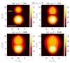 |
Fig. 3. Electron VDs at four different times along time evolution, showing the relaxation of the beam (cf. Fig. 5 in Ziebell et al. 2015). |
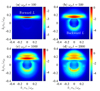 |
Fig. 4. Spectral intensity of Langmuir waves at four different times along time evolution, showing the forward L-mode excited by bump-on-tail instability (panel a) undergoing nonlinear scattering to produce backward L-mode as well (panel b; see Fig. 6 in Ziebell et al. (2015) for comparison). At later times (panels c and d), multiple scattering processes further spreads the L-mode spectrum in wave number space. |
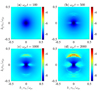 |
Fig. 5. Spectral intensity of ion-sound (S) waves at four different times along time evolution, indicating that S-mode excitation by decay instability is operative, but the intensity is rather low (cf. Fig. 7 in Ziebell et al. (2015)). |
where Fe(v) is normalized by ∫dvFe(v) = 1; e and me stand for the unit electric charge and the electron mass, respectively;  is the L-mode dispersion relation; ωpe = (4πnee2/me)1/2 is the plasma frequency, ne being the electron number density; the Debye length is given by
 ![Mathematical equation: $ \lambda_{De}=\left[T_{\mathrm{e}}/(4\pi n_{\mathrm{e}}e^2)\right]^{1/2}=v_{te}/\left(\sqrt{2}\omega_{pe}\right) $](/articles/aa/full_html/2025/04/aa53752-25/aa53752-25-eq11.gif) ; and
; and  is the L-mode wave intensity, defined via the total electrostatic electric field wave energy density,
  , where σ indicates forward (σ = 1) and backward (σ = −1) propagation along a given direction (conveniently chosen as the direction parallel to the electron beam propagation direction). Here,
  is the ion-acoustic (S) mode wave intensity, which is defined by the S-mode dispersion relation, ωkS = kcS(1+3Te/Ti)1/2(1+k2λD2)−1/2. Te and Ti are electron and ion temperatures, respectively, and vte = (2Te/me)1/2 and cS = (Te/mi)1/2 stand for the electron thermal and ion-sound speeds, respectively. The electric field spectral intensity for the transverse mode T is defined by
  , while the magnetic field intensity is given by
  . The linear dispersion relation for the T-mode is given by ωkT = (ωpe2+c2k2)1/2.
The wave intensities for plasma eigenmodes, namely, Langmuir (L), ion-sound (S), or equivalently, ion-acoustic, and transverse electromagnetic (T) modes, evolve according to the wave kinetic equations, which are displayed next. First, the L-mode wave kinetic equation is given by
![Mathematical equation: $$ \begin{aligned} \frac{\partial I_\mathbf{k}^{\sigma L}}{\partial t}&=\frac{4\pi e^2}{m_{\rm e}k^2}\int d\mathbf{v} \delta \left(\sigma \omega _\mathbf{k}^L-\mathbf{k}\cdot \mathbf{v}\right)\nonumber \\&\times \left(n_{\rm e}e^2F_{\rm e}(\mathbf{v}) +\pi \sigma \omega _\mathbf{k}^LI_\mathbf{k}^{\sigma L}\mathbf{k} \cdot \frac{\partial F_{\rm e}(\mathbf{v})}{\partial \mathbf{v}}\right) \nonumber \\&+\frac{\pi e^2}{2T_{\rm e}^2}\sum _{\sigma ^{\prime },\sigma ^{\prime \prime }=\pm 1} \int d\mathbf{k}^{\prime }\frac{\sigma \omega _\mathbf{k}^L (\mathbf{k}\cdot \mathbf{k}^{\prime })^2}{k^2{k^{\prime }}^2|\mathbf{k}-\mathbf{k}^{\prime }|^2} \left(\sigma \omega _\mathbf{k}^LI_{\mathbf{k}^{\prime }}^{\sigma ^{\prime }L} I_{\mathbf{k}-\mathbf{k}^{\prime }}^{\sigma ^{\prime \prime }S}\right. \nonumber \\&\left.-\sigma ^{\prime }\omega _{\mathbf{k}^{\prime }}^L I_{\mathbf{k}-\mathbf{k}^{\prime }}^{\sigma ^{\prime \prime }S}I_\mathbf{k}^{\sigma L} -\sigma ^{\prime \prime }\mu _{\mathbf{k}-\mathbf{k}^{\prime }}\omega _{\mathbf{k}-\mathbf{k}^{\prime }}^L I_{\mathbf{k}^{\prime }}^{\sigma ^{\prime }L}I_\mathbf{k}^{\sigma L}\right) \nonumber \\&\times \delta \left(\sigma \omega _\mathbf{k}^L -\sigma ^{\prime }\omega _{\mathbf{k}^{\prime }}^L -\sigma ^{\prime \prime }\omega _{\mathbf{k}-\mathbf{k}^{\prime }}^S\right) \nonumber \\&+\frac{e^2}{n_{\rm e}m_{\rm e}^2\omega _{pe}^2}\sum _{\sigma ^{\prime }}\int d\mathbf{k}^{\prime } \int d\mathbf{v}\frac{\sigma \omega _\mathbf{k}^L (\mathbf{k}\cdot \mathbf{k}^{\prime })^2}{k^2{k^{\prime }}^2} \nonumber \\&\times \left(\frac{n_{\rm e}e^2}{\omega _{pe}^2} \left(\sigma \omega _\mathbf{k}^LI_{\mathbf{k}^{\prime }}^{\sigma ^{\prime }L} -\sigma ^{\prime }\omega _{\mathbf{k}^{\prime }}^LI_\mathbf{k}^{\sigma L}\right) \left[F_{\rm e}(\mathbf{v})+F_i(\mathbf{v})\right]\right. \nonumber \\&\left.+\pi \frac{m_{\rm e}}{m_i}I_{\mathbf{k}^{\prime }}^{\sigma ^{\prime }L} I_\mathbf{k}^{\sigma L}(\mathbf{k}-\mathbf{k}^{\prime })\cdot \frac{\partial F_i(\mathbf{v})}{\partial \mathbf{v}}\right) \nonumber \\&\times \delta \left[\sigma \omega _\mathbf{k}^L -\sigma ^{\prime }\omega _{\mathbf{k}^{\prime }}^L-(\mathbf{k}-\mathbf{k}^{\prime })\cdot \mathbf{v}\right], \end{aligned} $$](/articles/aa/full_html/2025/04/aa53752-25/aa53752-25-eq17.gif) (10)
(10)
where μk = |k|3λDe3(me/mi)1/2(1+3Ti/Te)1/2. The term dictated by the linear wave-particle resonance delta-function δ(σωkL−k⋅v) defines the spontaneous and induced emission processes; the terms dictated by the three-wave delta-function resonance condition δ(σωkL−σ′ωk′L−σ″ωk − k′S) relate to the various nonlinear decay/coalescence processes among the plasma eigenmodes; and the terms associated with the nonlinear wave-particle resonance delta-function δ[σωkL−σ′ωk′L−(k−k′)⋅v] define the spontaneous and induced scattering processes. The proton distribution Fi is assumed to be stationary, and is given by a thermal distribution. The spontaneous emission term corresponds to the term proportional to Fe, while the induced emission is associated with ∂Fe/∂v. The spontaneous scattering term contains the factor Fe + Fi, while the induced scattering term is proportional to the derivative, ∂Fi/∂v.
The wave kinetic equation for the S-mode is given by
![Mathematical equation: $$ \begin{aligned} \frac{\partial }{\partial t}\frac{I_\mathbf{k}^{\sigma S}}{\mu _\mathbf{k}}&=\frac{4\pi \mu _\mathbf{k}e^2}{m_{\rm e}k^2} \int d\mathbf{v}\delta \left(\sigma \omega _\mathbf{k}^S-\mathbf{k}\cdot \mathbf{v}\right) \Biggl [n_{\rm e}e^2\left[F_{\rm e}(\mathbf{v})+F_i(\mathbf{v})\right] \nonumber \\&+\pi \sigma \omega _\mathbf{k}^L \frac{I_\mathbf{k}^{\sigma S}}{\mu _\mathbf{k}}\mathbf{k}\cdot \frac{\partial }{\partial \mathbf{v}}\left( F_{\rm e}(\mathbf{v})+\frac{m_{\rm e}}{m_i}F_i(\mathbf{v})\right)\Biggr ] \nonumber \\&+\frac{\pi e^2}{4T_{\rm e}^2}\sum _{\sigma ^{\prime },\sigma ^{\prime \prime }}\int d\mathbf{k}^{\prime } \frac{\sigma \omega _\mathbf{k}^L[\mathbf{k}^{\prime }\cdot (\mathbf{k}-\mathbf{k}^{\prime })]^2}{k^2{k^{\prime }}^2|\mathbf{k}-\mathbf{k}^{\prime }|^2} \nonumber \\&\times \left(\sigma \mu _\mathbf{k}\omega _\mathbf{k}^LI_{\mathbf{k}^{\prime }}^{\sigma ^{\prime }L} I_{\mathbf{k}-\mathbf{k}^{\prime }}^{\sigma ^{\prime \prime }L}-\sigma ^{\prime }\omega _{\mathbf{k}^{\prime }}^L I_{\mathbf{k}-\mathbf{k}^{\prime }}^{\sigma ^{\prime \prime }L}I_\mathbf{k}^{\sigma S} -\sigma ^{\prime \prime }\omega _{\mathbf{k}-\mathbf{k}^{\prime }}^L I_{\mathbf{k}^{\prime }}^{\sigma ^{\prime }L}I_\mathbf{k}^{\sigma S}\right) \nonumber \\&\times \delta \left(\sigma \omega _\mathbf{k}^S -\sigma ^{\prime }\omega _{\mathbf{k}^{\prime }}^L -\sigma ^{\prime \prime }\omega _{\mathbf{k}-\mathbf{k}^{\prime }}^L\right). \end{aligned} $$](/articles/aa/full_html/2025/04/aa53752-25/aa53752-25-eq18.gif) (11)
(11)
The first term on the right-hand side dictated by the velocity integral in equation (11) corresponds to the spontaneous and induced emissions of S-waves. These are depicted by the linear wave-particle resonance condition, δ(σωkS−k⋅v). The nonlinear terms are governed by the three-wave resonance condition δ(σωkS−σ′ωk′L−σ″ωk − k′S).
The T-mode wave kinetic equation is given by
![Mathematical equation: $$ \begin{aligned} \frac{\partial I_\mathbf{k}^{\sigma T}}{\partial t}&=\frac{\pi e^2}{32m_{\rm e}^2\omega _{pe}^2} \sum _{\sigma ^{\prime },\sigma ^{\prime \prime }}\int d\mathbf{k}^{\prime } \frac{\sigma \omega _\mathbf{k}^T(\mathbf{k}\times \mathbf{k}^{\prime })^2}{k^2{k^{\prime }}^2|\mathbf{k}-\mathbf{k}^{\prime }|^2} \nonumber \\&\times \left(\frac{k^{\prime 2}}{\sigma ^{\prime }\omega _{\mathbf{k}^{\prime }}^L} -\frac{|\mathbf{k}-\mathbf{k}^{\prime }|^2}{\sigma ^{\prime \prime } \omega _{\mathbf{k}-\mathbf{k}^{\prime }}^L}\right)^2\left( 2\sigma \omega _\mathbf{k}^TI_{\mathbf{k}^{\prime }}^{\sigma ^{\prime }L} I_{\mathbf{k}-\mathbf{k}^{\prime }}^{\sigma ^{\prime \prime }L}\right. \nonumber \\&\left.-\sigma ^{\prime }\omega _{\mathbf{k}^{\prime }}^L I_{\mathbf{k}-\mathbf{k}^{\prime }}^{\sigma ^{\prime \prime }L}I_\mathbf{k}^{\sigma T} -\sigma ^{\prime \prime }\omega _{\mathbf{k}-\mathbf{k}^{\prime }}^L I_{\mathbf{k}^{\prime }}^{\sigma ^{\prime }L}I_\mathbf{k}^{\sigma T}\right) \nonumber \\&\times \delta \left(\sigma \omega _\mathbf{k}^T -\sigma ^{\prime }\omega _{\mathbf{k}^{\prime }}^L -\sigma ^{\prime \prime }\omega _{\mathbf{k}-\mathbf{k}^{\prime }}^L\right) \nonumber \\&+\frac{\pi e^2}{4T_{\rm e}^2}\sum _{\sigma ^{\prime },\sigma ^{\prime \prime }}\int d\mathbf{k}^{\prime } \frac{\sigma \omega _\mathbf{k}^T(\mathbf{k}\times \mathbf{k}^{\prime })^2}{k^2{k^{\prime }}^2|\mathbf{k}-\mathbf{k}^{\prime }|^2} \left(2\sigma \omega _\mathbf{k}^TI_{\mathbf{k}^{\prime }}^{\sigma ^{\prime }L} I_{\mathbf{k}-\mathbf{k}^{\prime }}^{\sigma ^{\prime \prime }S}\right. \nonumber \\&\left.-\sigma ^{\prime }\omega _{\mathbf{k}^{\prime }}^L I_{\mathbf{k}-\mathbf{k}^{\prime }}^{\sigma ^{\prime \prime }S}I_\mathbf{k}^{\sigma T} -\sigma ^{\prime \prime }\mu _{\mathbf{k}-\mathbf{k}^{\prime }}\omega _{\mathbf{k}-\mathbf{k}^{\prime }}^L I_{\mathbf{k}^{\prime }}^{\sigma ^{\prime }L}I_\mathbf{k}^{\sigma T}\right) \nonumber \\&\times \delta \left(\sigma \omega _\mathbf{k}^T -\sigma ^{\prime }\omega _{\mathbf{k}^{\prime }}^L -\sigma ^{\prime \prime }\omega _{\mathbf{k}-\mathbf{k}^{\prime }}^S\right) \nonumber \\&+\frac{\pi e^2}{8m_{\rm e}^2}\sum _{\sigma ^{\prime },\sigma ^{\prime \prime }}\int d\mathbf{k}^{\prime } \frac{\sigma \omega _\mathbf{k}^T|\mathbf{k}-\mathbf{k}^{\prime }|^2}{(\omega _\mathbf{k}^T)^2 (\omega _{\mathbf{k}^{\prime }}^T)^2}\left(1 +\frac{(\mathbf{k}\cdot \mathbf{k}^{\prime })^2}{k^2{k^{\prime }}^2}\right) \nonumber \\&\times \left(2\sigma \omega _\mathbf{k}^TI_{\mathbf{k}^{\prime }}^{\sigma ^{\prime }T} I_{\mathbf{k}-\mathbf{k}^{\prime }}^{\sigma ^{\prime \prime }L} -2\sigma ^{\prime }\omega _{\mathbf{k}^{\prime }}^T I_{\mathbf{k}-\mathbf{k}^{\prime }}^{\sigma ^{\prime \prime }L}I_\mathbf{k}^{\sigma T} -\sigma ^{\prime \prime }\omega _{\mathbf{k}-\mathbf{k}^{\prime }}^L I_{\mathbf{k}^{\prime }}^{\sigma ^{\prime }T}I_\mathbf{k}^{\sigma T}\right) \nonumber \\&\times \delta \left(\sigma \omega _\mathbf{k}^T -\sigma ^{\prime }\omega _{\mathbf{k}^{\prime }}^T-\sigma ^{\prime \prime } \omega _{\mathbf{k}-\mathbf{k}^{\prime }}^L\right) \nonumber \\&+\frac{e^2}{2n_{\rm e}m_{\rm e}^2\omega _{pe}^2}\sum _{\sigma ^{\prime }} \int d\mathbf{k}^{\prime }\int d\mathbf{v}\frac{\sigma \omega _\mathbf{k}^T (\mathbf{k}\times \mathbf{k}^{\prime })^2}{k^2{k^{\prime }}^2} \nonumber \\&\times \left(\frac{n_{\rm e}e^2}{\omega _{pe}^2} \left(2\sigma \omega _\mathbf{k}^T I_{\mathbf{k}^{\prime }}^{\sigma ^{\prime }L} -\sigma ^{\prime }\omega _{\mathbf{k}^{\prime }}^L I_\mathbf{k}^{\sigma T}\right) \left[F_{\rm e}(\mathbf{v})+F_i(\mathbf{v})\right]\right. \nonumber \\&\left.+\frac{\pi m_{\rm e}}{m_i}I_{\mathbf{k}^{\prime }}^{\sigma ^{\prime }L} I_\mathbf{k}^{\sigma T}(\mathbf{k}-\mathbf{k}^{\prime })\cdot \frac{\partial F_i(\mathbf{v})}{\partial \mathbf{v}}\right) \nonumber \\&\times \delta \left[\sigma \omega _\mathbf{k}^T -\sigma ^{\prime }\omega _{\mathbf{k}^{\prime }}^L-(\mathbf{k}-\mathbf{k}^{\prime })\cdot \mathbf{v}\right]. \end{aligned} $$](/articles/aa/full_html/2025/04/aa53752-25/aa53752-25-eq19.gif) (12)
(12)
In the above, terms on the right-hand side dictated by the various three-wave resonant delta functions represent the decay/coalescence processes of various plasma eigenmodes. In particular, the coalescence of two L-modes into a T-mode at 2ωpe (L + L ↔ T) is responsible for the (second) harmonic emission. The decay of L-mode into an S-mode and a T-mode at the fundamental plasma frequency, ω ∼ ωpe, is one of the processes that are responsible for the fundamental emission (T ↔ L + S). The merging of a T-mode and an L-mode into the next higher harmonic T-mode (T ↔ T + L) is responsible for generating higher-harmonic plasma emission. The nonlinear wave-particle resonance process dictated by δ[σωkT−σ′ωk′L−(k−k′)⋅v] represents the spontaneous and induced scattering processes involving T and L-modes and the charged particles, ions and electrons (T ↔ p + L and T ↔ e + L). The process dictated by the nonlinear wave-particle resonance σωkT − σ′ωk′L − (k − k′) ⋅ v = 0 represents an alternative mechanism for the fundamental emission.
The complete numerical solution of coupled equations (9)–(12) provides snapshots of various physical quantities at successive time steps during their time evolution, for example, the overall time evolution of integrated wave intensities for each wave mode. We note that Ziebell et al. (2015) have indeed accomplished the task of obtaining a full numerical solution for the first time, which has been spectacularly confirmed by the full two-dimensional particle-in-cell (PIC) simulation (Lee et al. 2019). New dynamic radio spectra can be calculated along a certain direction of propagation using the intensity of T-waves integrated in the wave vector space. In the present paper, we make use of the numerical solution, as in Ziebell et al. (2015), and compute the synthetic radio dynamic spectrum by integrating in the wave vector space, while repeating the computation at fixed spatial locations along the propagation paths of the radio source.
3.2. Interlude
In observations, the time/space drift of radio spectra is governed by the variation of plasma density with distance from the Sun, see Sect. 2, which we also use to simulate such spectra. Rough estimates from the observed spectra indicate different time intervals for these drifts/variations, which are on the order of tens of minutes or hours in the case of type II emissions, and smaller on the order of tens of seconds or minutes for type III ones. These time intervals are, in general, long enough compared to the characteristic times of instability saturation or to those of radio emissions, which are generally much under 1 s.
On the other hand, the QL or PIC simulations show that the core-beam configuration changes (relaxes) with time, involving a more gentle bump-on-tail or even a plateau-on-tail distribution, which can be robust enough to sustain a long radiative process, but is in general insufficient to address Sturrock’s dilemma (Sturrock 1964), in spite of the recent model in Sauer et al. (2019). However, studies involving the propagation of an electron beam of finite source size or the electron beam traveling in an inhomogeneous plasma have shown that the beam reformation is sufficient to overcome the rapid relaxation of the beam (Takakura & Shibahashi 1976; Magelssen & Smith 1977; Mel’nik et al. 1999; Kontar & Pécseli 2002; Foroutan et al. 2007; Ratcliffe et al. 2012; Voshchepynets et al. 2015), thus allowing the nonlinear generation of radio waves, which can persist even after the plateau is established. The observations support the robustness of the bump-on-tail or even plateau-on-tails, and their association with plasma excitation of type III bursts (Ergun et al. 1998).
We invoke these aspects to motivate an iteration of the WT simulation at successive time steps (much shorter than drifting intervals from the observations), and with a decreasing electron (total) density (and a decreasing plasma frequency) corresponding to an increasing distance from the Sun. Before presenting the synthetic dynamic radio spectra for type II and type III sources, which we have generated via this method, let us first overview the result of a sample WT simulation carried out at one source location, which is discussed next.
3.3. Local WT simulation
In order to illustrate the time evolution of the beam plasma instability and the ensuing emission of transverse waves by nonlinear plasma processes, we make use of some results in the paper by Ziebell et al. (2015), which aimed to elucidate details of the physical mechanisms associated with plasma emission, as described by WT theory. Thus, Ziebell et al. (2015) computed the time evolution of waves and particles triggered by an electron beam propagating in the background of a Maxwellian plasma. The relative beam-to-background electron number density was assumed to be nb/n0 = 1 × 10⁻³, with a plasma parameter of 1/(n0λD3) = 5 × 10⁻³ and the thermal velocity of the background electrons as vte2/c2 = 4.0 × 10⁻³. Different values of the beam speed were considered, but here we only show the results obtained in one of these cases, that is, when the beam velocity was 8 times the electron thermal velocity, Vb/vte = 8. Figure 3 displays contour plots of the electron VD as a function of normalized parallel and perpendicular velocities. Panel (a) clearly shows the presence of the background and beam populations at a relatively early time, and panels (b), (c), and (d) show different stages of the time evolution, with gradual relaxation and the final formation of a broad plateau in the VD. Figure 3 is basically the same as Fig. 5 of Ziebell et al. (2015).
Figures 4 and 5 display the corresponding contour plots of the wave intensity for Langmuir (L) and ion-sound (S) waves, respectively. The primary peak of Langmuir waves (forward L) induced by the bump-on-tail instability is already formed in Fig. 4, panel (a). Panel (b) shows the broadening of the primary peak and the appearance of the peak corresponding to backward propagating waves (backward L), as well as the initial steps of the formation of a ring-like structure in wavenumber space, due to scattering and decay processes. Panels (c) and (d) illustrate subsequent moments of the wave evolution, characterized mainly by the broadening of the peaks in the L-wave spectrum, with the formation of some structures in the main peaks. The corresponding spectrum of S-waves is shown in the four panels of Fig. 5. Some structures appear in the spectrum but are not as conspicuous as those in the L spectrum seen in Fig. 4. The overall intensity of the S-mode is quite modest, as evidenced by Fig. 5.
Figure 6 depicts images of the spectrum for transverse (T) waves. The spectrum of T-waves has a fundamental difference relative to the L and S spectra, based on the fact that it is assumed to be nonexistent at the start of the time evolution, while the L and S spectra start from an initial value which satisfies the balance between spontaneous and induced emissions, in an initial Maxwellian plasma. With the injection of the beam, the system starts to evolve, and nonlinear processes involving L and S-waves start to generate T-waves. In Fig. 6, panel (a), the T-mode is already formed at (normalized) time τ = tωpe = 100, with an intensity level similar to that of the S-waves. At τ = 500 in panel (b), a peak is developed at k ≃ 0 (corresponding to ω ≃ ωpe, the fundamental emission), and some structure starts to appear, forming a ring in the wavenumber space. The intensity of waves in this ring, integrated along the solid angle, corresponds to a peak at ω ≃ 2ωpe, the second harmonic emission. These features become more prominent and appear to be well established at τ = 1000, as shown in Fig. 6, panel (c). For later times, as for τ = 2000 depicted in panel (d), the fundamental peak is similar to that appearing in panel (c), the harmonic ring is more intense, and there occurs even emission of the third harmonic corresponding to n = 3, albeit with lower intensity.
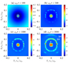 |
Fig. 6. Spectral intensity of transverse waves at four different times along time evolution, as in Fig. 8 in Ziebell et al. (2015). |
3.4. Dynamic spectra from WT simulations
The formalism already described in Sect. 3.3 to obtain the time evolution of waves and particles at a certain spatial point, using the WT theory, is utilized to describe the evolution in an inhomogeneous system, intended to simulate the solar wind environment. We consider a plasma with uniform temperature, but decreasing density, proportional to (Rs/R)2, as the distance R from the Sun increases, where Rs is the solar radius (see Sect. 2). Our methodology relies on the models schematized in Fig. 7, for two distinct situations. One is that of a flare-generated electron beam propagating away from the Sun, along open magnetic field lines, primarily along the radial direction. This is depicted in Fig. 7 as the source of type III radio bursts. The second situation considered is that of a plasma “blob” meant to represent a traveling coronal mass ejecta or CME propagating away from the Sun along the radial direction. The beam of electrons is accelerated along the CME shock surface, in directions parallel and antiparallel to the local magnetic field lines, which are directed perpendicular to the radial expansion direction. The second case is also depicted in Fig. 7 as a source of type II radio emission slowly expanding in the radial direction with speed Vs ≃ VCME, which is substantially lower than Vb. We consider a series of points along the radial distance between R = 1Rs and R = 6Rs. The WT theory (Sect. 3.1) is applied at each point along the radial path, with different background densities, locally generating results similar to those depicted in Sect. 3.3. In doing so, we have neglected space-dependent mechanisms such as spatial diffusion, which are assumed to be less relevant than those taken into account in the formulation presented in Sect. 3.1.
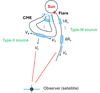 |
Fig. 7. Cartoon representation of type II and type III radio sources moving from R = Rs to R = 6Rs, which is the range over which the WT simulation is applied. For the type III source traveling along open magnetic field lines, the source velocity is given by the beam velocity, Vs ≃ Vb. For the type II source, while the electron beam is accelerated at the shock front (with average speeds ±Vb), the traveling speed of the source itself is much lower, Vs ≃ VCME ≪ Vb. |
The protons in the plasma medium are assumed to have a Maxwellian distribution, which remains unchanged. The background electrons are described by a Maxwellian core plus a Kappa halo, and the beam injected into the system at τ = 0 is assumed to be a drifting Maxwellian with the same thermal velocity vte as the background population. In 3D, the electron distribution function is as equation (1) of Ziebell (2021). The Kappa population is assumed to have a relative density 5.0 × 10⁻² and a kappa index κe = 5.0, to simulate the suprathermal feature of electron populations, frequently observed in the solar wind. This is distinct from the original paper of Ziebell et al. (2015), where all populations of electrons and protons are simply considered Maxwellian. However, we still assume the same parametrization from Sect. 3.3, also as in Ziebell et al. (2015): 1/(n0λD3) = 5 × 10⁻³, vte2/c2 = 4.0 × 10⁻³, Vb = 8vte, and the relative beam density at S = R/Rs = 1 is nb/ne = 5.0 × 10⁻⁴.
In the numerical analysis, we have considered two-dimensional (2D) spaces for wave number and velocity, and transformed the kinetic equations into finite difference equations. The equation for the time evolution of the VD function of electrons is solved using the splitting method, and the wave equations are solved using a fourth-order Runge-Kutta method with (normalized) time interval Δτ = 0.1, where τ = ωpe*t, ωpe* being the plasma frequency at S = 1. This is the same numerical scheme used in Ziebell et al. (2015). For the wave equations, we utilized 39×39 grids for 0 < q⊥ = k⊥vte/ωpe* < 0.4, and 0 < q∥ = k∥vte/ωpe* < 0.4. For the particle equation, we use a 51×101 grid for 0 < u⊥ = v⊥/vte < 15 (perpendicular velocity) and −15 < uz = v∥/vte < 15 (parallel velocity). The radial distance has been represented by a grid of 25 points, evenly spaced between R = 1Rs and R = 6Rs.
The use of the results obtained by WT theory for the generation of synthetic spectra depends on the time of beam propagation. For type III emission, we can consider that the beam travels along the radial direction for simplicity. We have assumed the beam velocity Vb = 8vte, so that Vb = 1.5 × 10⁸ m/s (or energies of about 64 keV).2 This means that the beam covers the distance between S = 1 and S = 6 in about 20 s. The times of evolution of the radiative mechanisms leading to radio emissions, as described by the WT theory, are much shorter than the beam travel time. This implies, for instance, that the T-waves are fully developed at S = 2 well before the beam arrives at S = 6. As a consequence, a distant observer receives the transverse waves generated at low values of S before it receives the waves generated at larger values of S. In short, the time delay between waves generated at different distances depends on the source velocity, as already discussed in Sect. 2.
Figure 8 shows the 1D electron VD function, that is, the electron distribution integrated along u⊥, as a function of uz and dimensionless radial distance, S = R/Rs, at two (normalized) times, τ = ωpe*t = 200 (upper) and τ = ωpe*t = 500 (lower). Thus, the transformations undergone by the VDs at these two instants, under the effect of the wave excitations, suggest a slightly faster relaxation of the electron beam at larger distances. In the time intervals characteristic of radio emissions, for example, of the fundamental and second harmonic components, this relaxation leads to the flattening of the beam, with a slightly wider flattening at the radial distance of S = 6 compared to S = 1. These times are much below 1 s; for instance, the relaxation time (at local plasma frequency) is t ∼ 500/ωpe* ≤ 10−6 s at S = 1, t ∼ 500/ωpe ≤ 10−5 s at S = 6, and t ∼ 500/ωpe ≤ 5 ⋅ 10−3 s at R = 1 AU, which means at S ≃ 215. It is seen that these times are all much shorter than the beam propagation timescales between the two positions considered here, for example, t ≃ 20 s for type III emissions and t ≃ 200 s for type II emissions. In addition, the radiative times are still small enough compared to the steps δt representing the beam travel time between the discrete positions along radial distance, δt ≃ Rs/Vb/5 ≃ 1.0 s. This also allows us to assume that the diffusive processes under the action of the (self-generated) electrostatic turbulence are fast enough to contribute to the fast and efficient acceleration and restoration of the electron beams during the same intervals δt (Ratcliffe et al. 2012).
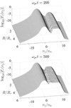 |
Fig. 8. 1D VD (integrated along v⊥) as a function of (normalized) distance R/Rs, for ωpet = 200 (upper) and ωpet = 500 (lower). |
Figure 9 displays the transverse wave spectra versus the normalized wave number q = kvte/ωpe* and the normalized distance S, for τ = 500. Both the fundamental and harmonic peaks obtained at different spatial positions are already well developed at this instant in the time evolution. The 2D spectrum of wave intensities Ik⊥, k∥σT is converted into a function depending on k = (k⊥2 + k∥2)1/2 and azimuthal angle φ,  , and then integrated over φ to obtain
  or the normalized wave intensity defined as
  (see legend). The same spectra can be computed to show
  as a function of the normalized wave frequency zqT = ωqT/ωpe* corresponding to the value of q. The component F shows a localized intensity peak (red) at S ≃ 4, which appears to be only a numerical artifact, without physical significance.3 For the type III source, since the beam excites nonlinear processes leading to emission of transverse waves, the velocity of the source of these waves coincides with the beam velocity. The time delay between T-waves generated at S = 1 (or R = Rs) and S = 6 (or R = 6Rs) is about 20 s, as already mentioned. This can be seen in Fig. 10, where the color-coded intensity spectra of T-waves are computed as in Fig. 9, but for τ = 1000 (for each point of emission) and as a function of the normalized wave frequency zq = ω/ωpe* and the delay time, t(s) = ΔR/Vb = RsΔS/Vb. These waves appear in Fig. 10 in the form of two narrow bands with steep gradients, concentrated in the region t ≤ 20 s. The lower band corresponds to the fundamental emission, and the upper band to the second harmonic emission. In Fig. 10, and also the next Fig. 11, the synthetic spectra of type II and type III emissions are not connected to each other, as in the case of those often reported by observations, which are linked to the same coronal event. However, we show the two types of spectra in the same panel in order to emphasize the similarity with the theoretical profiles in Fig. 2 and with the observations in Fig. 1.
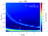 |
Fig. 9. Intensity spectra of T-waves (see text), as a function of the normalized wave number and space position, for τ = 500. |
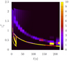 |
Fig. 10. Color-coded synthetic dynamic spectra of T-waves computed as in Fig. 9, but for τ = 1000 and as a function of the normalized wave frequency and delay time. The color scale represents the normalized wave intensity |

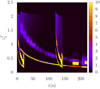 |
Fig. 11. Color-coded synthetic dynamic spectra of T-waves ( |

For the second case of a type II source, with a velocity much lower than the beam velocity, Vs ≪ Vb, the time delay of the generated waves will then be correspondingly longer. We keep the already mentioned value of the beam velocity (Vb = 0.5c), which seems exaggerated for electrons at the origin of type II emission but is still less demanding in the numerical calculation. However, observations suggest that type II and herringbone electrons in the low corona up to 2–3Rs can be accelerated by the shock drift acceleration mechanism producing electron beams with energies up to 80 keV, which correspond to a limit beam velocity Vbl ≃ 0.57c (see e.g., Mann & Klassen (2005), Mann et al. (2018)). The results in Fig. 10 are generated by assuming that the source has Vs = Vb/10 = 0.8vte. For this configuration, the spectrum of waves generated in Fig. 10 as a relatively broad curved band extending from t ≃ 0 to t ≃ 250 s, corresponds to the broad band of harmonic waves and below a thinner band of fundamental emission. Despite the differences in the timescales, we can still find a direct correspondence between the spectra in Figs. 10 and 2, especially with the descending dynamic spectra, which include the lowest frequencies measured in situ (e.g., at 1 AU), as in Figs. 1 and 2 – also similar to Fig. 1 in Schmidt et al. (2013). For observers in the vicinity of Earth, such as satellites (e.g., Wind or STEREO A/B), we can extend the path of the radio sources to almost 1 AU ≃ 215RS. For the same parametrization of plasma radio sources assumed here, the delay times will increase to t ≃ 16 min for type III spectra, and t ≃ 160 min for type II spectra, which are consistent (comparable) with the time intervals in Fig. 2.
Finally, in Fig. 11 we demonstrate that our methodology can also produce multiple time-distinct dynamic spectra, as often reported by observations (Ergun et al. 1998; Schmidt et al. 2013; Reid & Ratcliffe 2014; Nedal et al. 2023). Thus, in addition to the two situations considered to generate the spectra in Fig. 10, we consider the emission of a second beam moving along the radial direction, at a time assumed to be 120 s after the emission of the first beam. Figure 11 shows the outcome of this simulation, with an additional pair of type III bands, compared to the bands obtained in Fig. 10. This depiction is purely hypothetical, and the purpose is to compare with a situation where another flare-generated type III bursts follow the original set of type II/III radio emission. Multiple type III emissions are quite often present in observational data, being detected widely separated in time intervals, and our purpose was to reproduce one such situation (see, e.g., Fig. 1 in Schmidt et al. (2013)).
4. Conclusions and further prospects
The study of radio emissions is fully motivated by the information carried, often a unique way to remotely diagnose their plasma sources. For this, a realistic modeling of both the radiative processes and the propagation of radio emissions is needed, as they are revealed by the dynamic spectra of type II and type III radio bursts generated by energetic solar events. On the one hand, understanding of type II and type III radio emissions is therefore particularly important in the context of space weather, for forecasting solar events, such as CMEs and coronal flares, and subsequent SEPs. On the other hand, space missions can measure in situ providing unique counterparts of their plasma sources, which are vital for building realistic models of radiative plasma processes, as well as realistic synthetic spectra.
Here we have proposed a novel method to reproduce the dynamic spectra of the solar radio bursts of type II and type III, using WT theory. The intensities of the radio emissions were self-consistently and quantitatively evaluated on the basis of first-principles modeling of electron beam plasma instabilities and nonlinear wave interaction. These values are computed iteratively and associated with the frequency of EM waves, which decreases with the distance or propagation time of their plasma sources. The difference in the descending frequency drift is caused by the speed of these sources. For type III bursts, it is the speed of the energetic beams, and in the case of type II emissions, it is approximately given by the lower speed of the interplanetary shock triggered, for instance, by a CME. For each radio burst, not only the fundamental emission but also the second harmonic have been computed, the latter having a dynamic spectrum of a wider band.
The examples of dynamic spectra presented here as preliminary results were computed for short distances in the solar corona, between R = 1 RS and R = 6RS. This is motivated by the fact that this first analysis is limited to the main elements in the modeling of these spectra, such as the reproduction of the descending temporal (spatial) profile of the frequency and also to the calculation of the intensity of radio emissions using the WT theory. Other effects, such as the absorption or scattering suffered by the primary (quasilinear) and secondary (nonlinear) wave emissions, or the more pronounced relaxations of the electron beams, are not considered in our present computations. In this way, we could assume that the dispersion relations of the wave emissions do not undergo major changes. However, the action of some effects such as these is not excluded because we invoked them, for example in the restoration of electron beams, which is sufficiently plausible at the timescales considered here.
We have also shown that these simplified models can be expanded to reproduce dynamic spectra captured at larger distances or propagation times of their plasma sources, such as those measured by the satellites Wind and STEREO-A/B at 1 AU. Such extended models of dynamic radio spectra will be addressed in future studies, and it is very likely that they will take into account additional effects, such as those already mentioned. Moreover, present findings demonstrate that our theoretical approach based on WT theory can be further developed to obtain quantitatively relevant replications but also valuable predictions of the observed dynamic spectra of radio bursts. In the context of space weather forecasting, including the consequences of energetic solar events, our results can also contribute to improved large-scale models of the solar radio sources based on first-principle approaches, which are otherwise computed from the large-scale MHD simulations or even from direct spacecraft observations.
This is the radial density profile from the Parker (1958) model of the solar wind with spherically symmetric expansion and constant velocity. Observations of the solar wind, and also the density of a quiet solar corona, often conform well enough to this radial profile (Vocks et al. 2018). Other profiles can also be invoked, either less steep specific to high solar activity (when the density at large coronal heights increases), or steeper profiles from hydrostatic models (Harding et al. 2019).
Apparently high, this value is still in the range of measurements during impulsive events that can be at the origin of type III emissions, when the electron energies can reach up to a few hundred keV (Lin 1997; Klassen et al. 2011; Gómez-Herrero et al. 2021).
Other lower intensity peaks can also be identified at different distances, suggesting a link with the discreteness of the grid points in velocity and wave number spaces, which do not always coincide with the resonance condition (changing with the evolution of electron beam) in QL theory. Future studies should refine these calculations to obtain smoother numerical spectra, for example by implementing denser grids, which currently require much more computer time.
Acknowledgments
The authors acknowledge support from the Katholieke Universiteit Leuven and the Ruhr-University Bochum. LFZ acknowledges support from CNPq (Brazil), grant No. 303189/2022-3, and partial support by Coordenação de Aperfeiçoamento de Pessoal de Nível Superior – Brasil (CAPES) – Finance Code 001. PHY was supported by NASA Grant 80NSSC23K0662, NSF Grant 2203321, and the Department of Energy (DOE DE-SC0022963) through the NSF/DOE Partnership in Basic Plasma Science and Engineering. These results were also obtained in the framework of the projects C16/24/010 (C1 project Internal Funds KU Leuven), G002523N (FWO-Vlaanderen), 4000145223 SIDC Data Exploitation (SIDEX2), ESA Prodex, Belspo project B2/191/P1/SWiM.
References
- Adhikari, L., Zank, G. P., Hu, Q., & Dosch, A. 2014, ApJ, 793, 52 [Google Scholar]
- Bacchini, F., & Philippov, A. A. 2024, MNRAS, 529, 169 [Google Scholar]
- Bale, S. D., Reiner, M. J., Bougeret, J. L., et al. 1999, GRL, 26, 1573 [Google Scholar]
- Cairns, I. H., Knock, S. A., Robinson, P. A., & Kunic, Z. 2003, Space Sci. Rev., 107, 27 [NASA ADS] [CrossRef] [Google Scholar]
- Davidson, R. C. 1972, Methods in Nonlinear Plasma Theory (New York: Academic Press) [Google Scholar]
- Ergun, R. E., Larson, D., Lin, R. P., et al. 1998, ApJ, 503, 435 [NASA ADS] [CrossRef] [Google Scholar]
- Foroutan, G. R., Robinson, P. A., Sobhanian, S., et al. 2007, Phys. Plasmas, 14, 012903 [Google Scholar]
- Gómez-Herrero, R., Pacheco, D., Kollhoff, A., et al. 2021, A&A, 656, L3 [NASA ADS] [CrossRef] [EDP Sciences] [Google Scholar]
- Gopalswamy, N., Aguilar-Rodrigues, E., Yashiro, S., et al. 2005, JGR, 110, A12S07 [Google Scholar]
- Harding, J. C., Cairns, I. H., & Lobzin, V. V. 2019, ApJ, 877, 25 [Google Scholar]
- Hegedus, A. M., Manchester, W. B., & Kasper, J. C. 2021, ApJ, 922, 203 [NASA ADS] [CrossRef] [Google Scholar]
- Henri, P., Sgattoni, A., Briand, C., Amiranoff, F., & Riconda, C. 2019, JGR (Space Phys.), 124, 1475 [Google Scholar]
- Klassen, A., Gómez-Herrero, R., & Heber, B. 2011, Sol. Phys., 273, 413 [NASA ADS] [CrossRef] [Google Scholar]
- Kontar, E. P., & Pécseli, H. L. 2002, Phys. Rev. E, 65, 066408 [Google Scholar]
- Kumari, A., Morosan, D. E., Kilpua, E. K. J., & Daei, F. 2023, A&A, 675, A102 [NASA ADS] [CrossRef] [EDP Sciences] [Google Scholar]
- Lazar, M., López, R. A., Poedts, S., & Shaaban, S. M. 2023, Sol. Phys., 298, 72 [Google Scholar]
- Lee, S.-Y., Ziebell, L. F., Yoon, P. H., Gaelzer, R., & Lee, E. S. 2019, ApJ, 871, 74 [NASA ADS] [CrossRef] [Google Scholar]
- Lee, S.-Y., Yoon, P. H., Lee, E., & Tu, W. 2022, ApJ, 924, 36 [NASA ADS] [CrossRef] [Google Scholar]
- Li, B., & Cairns, I. H. 2013a, ApJ, 763, L34 [Google Scholar]
- Li, B., & Cairns, I. H. 2013b, JGR (Space Phys.), 118, 4748 [Google Scholar]
- Li, B., & Cairns, I. H. 2014, Sol. Phys., 289, 951 [Google Scholar]
- Li, B., Cairns, I. H., & Robinson, P. A. 2008a, JGR (Space Phys.), 113, A06104 [Google Scholar]
- Li, B., Cairns, I. H., & Robinson, P. A. 2008b, JGR (Space Phys.), 113, A06105 [Google Scholar]
- Lin, R. P. 1997, in Coronal Physics from Radio and Space Observations, ed. G. Trottet, 483, 93 [Google Scholar]
- Lin, R. P., Potter, D. W., Gurnett, D. A., & Scarf, F. L. 1981, ApJ, 251, 364 [NASA ADS] [CrossRef] [Google Scholar]
- Magdalenic, J., Marqué, C., Krupar, V., et al. 2014, ApJ, 791, 115 [Google Scholar]
- Magelssen, G. R., & Smith, D. F. 1977, Solar Phys., 55, 211 [Google Scholar]
- Mäkelä, P., Gopalswamy, N., Reiner, M. J., Akiyama, S., & Krupar, V. 2016, ApJ, 827, 141 [Google Scholar]
- Manini, F., Cremades, H., López, F. M., & Nieves-Chinchilla, T. 2023, Sol. Phys., 298, 145 [Google Scholar]
- Mann, G., & Klassen, A. 2005, A&A, 441, 319 [NASA ADS] [CrossRef] [EDP Sciences] [Google Scholar]
- Mann, G., Melnik, V. N., Rucker, H. O., Konovalenko, A. A., & Brazhenko, A. I. 2018, A&A, 609, A41 [NASA ADS] [CrossRef] [EDP Sciences] [Google Scholar]
- McLean, D. J., & Labrum, N. R. 1985, Solar Radiophysics (Cambridge: Cambridge University Press) [Google Scholar]
- Mel’nik, V. N., Lapshin, V., & Kontar, E. 1999, Sol. Phys., 184, 353 [CrossRef] [Google Scholar]
- Melrose, D. B. 1980, Plasma Astrophysics (New York: Gordon and Breacj) [Google Scholar]
- Melrose, D. B. 2008, Proc. Int. Astron. Union, 4, 305 [Google Scholar]
- Ndacyayisenga, T., Uwamahoro, J., Uwamahoro, J. C., Kwisanga, C., & Monstein, C. 2025, ASR, 75, 1415 [Google Scholar]
- Nedal, M., Kozarev, K., Zhang, P., & Zucca, P. 2023, A&A, 680, A106 [NASA ADS] [CrossRef] [EDP Sciences] [Google Scholar]
- Parker, E. N. 1958, ApJ, 128, 664 [Google Scholar]
- Pulupa, M., & Bale, S. D. 2008, ApJ, 676, 1330 [NASA ADS] [CrossRef] [Google Scholar]
- Pulupa, M. P., Bale, S. D., & Kasper, J. C. 2010, JGR (Space Phys.), 115, A04106 [Google Scholar]
- Ratcliffe, H., Bian, N. H., & Kontar, E. P. 2012, ApJ, 761, 176 [Google Scholar]
- Reames, D. V. 2021, Solar Energetic Particles: A Modern Primer on Understanding Sources, Acceleration and Propagation, The Lecture Notes in Physics (Heidelberg: Springer) [CrossRef] [Google Scholar]
- Reid, H. A. S., & Ratcliffe, H. 2014, RAA, 14, 773 [NASA ADS] [Google Scholar]
- Richardson, J. D. 2010, in Heliophysical Processes, eds. N. Gopalswamy, S. Hasan, & A. Ambastha (Berlin, Heidelberg: Springer, Berlin Heidelberg), 83 [CrossRef] [Google Scholar]
- Richardson, I. G., Mays, M. L., & Thompson, B. J. 2018, Space Weather, 16, 1862 [CrossRef] [Google Scholar]
- Roberts, J. A. 1959, Austr. J. Phys., 12, 327 [Google Scholar]
- Sagdeev, R. Z., & Galeev, A. A. 1969, Nonlinear Plasma Theory (New York: Benjamin) [Google Scholar]
- Sauer, K., Baumgärtel, K., Sydora, R., & Winterhalter, D. 2019, JGR (Space Phys.), 124, 68 [Google Scholar]
- Schmidt, J. M., & Cairns, I. H. 2012a, JGR (Space Phys.), 117, A04106 [Google Scholar]
- Schmidt, J. M., & Cairns, I. H. 2012b, JGR (Space Phys.), 117, A11104 [Google Scholar]
- Schmidt, J. M., & Cairns, I. H. 2014, JGR (Space Phys.), 119, 69 [Google Scholar]
- Schmidt, J. M., & Cairns, I. H. 2016, GRL, 43, 50 [Google Scholar]
- Schmidt, J. M., Cairns, I. H., & Hillan, D. S. 2013, ApJ, 773, L30 [Google Scholar]
- Sturrock, P. 1964, WN Hess (NASA, SP-50), 357 [Google Scholar]
- Takakura, T., & Shibahashi, H. 1976, Sol. Phys., 46, 323 [Google Scholar]
- Thejappa, G., MacDowall, R. J., & Bergamo, M. 2012, JGR (Space Phys.), 117 [Google Scholar]
- Vocks, C., Mann, G., Breitling, F., et al. 2018, A&A, 614, A54 [NASA ADS] [CrossRef] [EDP Sciences] [Google Scholar]
- Voshchepynets, A., Krasnselskikh, V., Artemyev, A., & Volokitin, A. 2015, ApJ, 807, 38 [NASA ADS] [CrossRef] [Google Scholar]
- Wild, J. P. 1950, Aust. J. Sci. Res. Phys. Sci., 3, 541 [NASA ADS] [Google Scholar]
- Yoon, P. H. 2006, Phys. Plasmas, 13, 022301 [Google Scholar]
- Yoon, P. H. 2019, Classical Kinetic Theory of Weakly Turbulent Nonlinear Plasma Processes (Cambridge University Press) [Google Scholar]
- Yoon, P. H., Ziebell, L. F., Gaelzer, R., & Pavan, J. 2012, Phys. Plasmas, 19, 102303 [Google Scholar]
- Ziebell, L. F. 2021, Ap&SS, 366, 60 [Google Scholar]
- Ziebell, L. F., Yoon, P. H., Gaelzer, R., & Pavan, J. 2014, ApJ, 795, L32 [Google Scholar]
- Ziebell, L. F., Yoon, P. H., Petruzzellis, L. T., Gaelzer, R., & Pavan, J. 2015, ApJ, 806, 237 [Google Scholar]
- Ziebell, L. F., Petruzzellis, L. T., Yoon, P. H., Gaelzer, R., & Pavan, J. 2016, ApJ, 818, 61 [Google Scholar]
All Figures
|
Fig. 1. Dynamic spectra from the WAVES experiment on Wind (upper panels) and GOES-10 soft X-ray flux data (bottom panel). A flare at 22:09:11 UT on August 24, 1998, is associated with an abrupt onset of soft X-ray flux and the intense type III burst, while the type II burst has a slow frequency-drifting feature, preceding the IP shock generated by the CME. After Bale et al. (1999). |
| In the text | |
|
Fig. 2. Frequency downshift from Eqs. (2)–(4) for type III and type II spectra, with, respectively, the following parameters: τE = 42 and 840 min, t0 = 115 and 135 min, and η = 0.02 and 0.035. There is agreement of these profiles with the spectra in Fig. 1, and Fig. 1 in Schmidt et al. (2013). |
| In the text | |
|
Fig. 3. Electron VDs at four different times along time evolution, showing the relaxation of the beam (cf. Fig. 5 in Ziebell et al. 2015). |
| In the text | |
|
Fig. 4. Spectral intensity of Langmuir waves at four different times along time evolution, showing the forward L-mode excited by bump-on-tail instability (panel a) undergoing nonlinear scattering to produce backward L-mode as well (panel b; see Fig. 6 in Ziebell et al. (2015) for comparison). At later times (panels c and d), multiple scattering processes further spreads the L-mode spectrum in wave number space. |
| In the text | |
|
Fig. 5. Spectral intensity of ion-sound (S) waves at four different times along time evolution, indicating that S-mode excitation by decay instability is operative, but the intensity is rather low (cf. Fig. 7 in Ziebell et al. (2015)). |
| In the text | |
|
Fig. 6. Spectral intensity of transverse waves at four different times along time evolution, as in Fig. 8 in Ziebell et al. (2015). |
| In the text | |
|
Fig. 7. Cartoon representation of type II and type III radio sources moving from R = Rs to R = 6Rs, which is the range over which the WT simulation is applied. For the type III source traveling along open magnetic field lines, the source velocity is given by the beam velocity, Vs ≃ Vb. For the type II source, while the electron beam is accelerated at the shock front (with average speeds ±Vb), the traveling speed of the source itself is much lower, Vs ≃ VCME ≪ Vb. |
| In the text | |
|
Fig. 8. 1D VD (integrated along v⊥) as a function of (normalized) distance R/Rs, for ωpet = 200 (upper) and ωpet = 500 (lower). |
| In the text | |
|
Fig. 9. Intensity spectra of T-waves (see text), as a function of the normalized wave number and space position, for τ = 500. |
| In the text | |
|
Fig. 10. Color-coded synthetic dynamic spectra of T-waves computed as in Fig. 9, but for τ = 1000 and as a function of the normalized wave frequency and delay time. The color scale represents the normalized wave intensity |
| In the text | |
|
Fig. 11. Color-coded synthetic dynamic spectra of T-waves ( |
| In the text | |
Current usage metrics show cumulative count of Article Views (full-text article views including HTML views, PDF and ePub downloads, according to the available data) and Abstracts Views on Vision4Press platform.
Data correspond to usage on the plateform after 2015. The current usage metrics is available 48-96 hours after online publication and is updated daily on week days.
Initial download of the metrics may take a while.