| Issue |
A&A
Volume 660, April 2022
|
|
|---|---|---|
| Article Number | A139 | |
| Number of page(s) | 12 | |
| Section | Cosmology (including clusters of galaxies) | |
| DOI | https://doi.org/10.1051/0004-6361/202141909 | |
| Published online | 26 April 2022 | |
CMASS galaxy sample and the ontological status of the cosmological principle
1
Department of Astronomy and Atmospheric Sciences, Kyungpook National University, Daegu 41566, Republic of Korea
2
Division of Science Education and Institute of Science Education, Jeonbuk National University, Jeonju 54896, Republic of Korea
e-mail: This email address is being protected from spambots. You need JavaScript enabled to view it.
3
Theoretical Astrophysics Group, Korea Astronomy and Space Science Institute, Daejeon 34055, Republic of Korea
4
Center for Theoretical Physics of the Universe, Institute for Basic Science (IBS), 55, Expo-ro, Yuseong-gu, Daejeon 34126, Republic of Korea
Received:
30
July
2021
Accepted:
10
January
2022
Abstract
Context. The cosmological principle (CP), assuming spatially homogeneous and isotropic background geometry in the cosmological scale, is a fundamental assumption in modern cosmology. Recent observations of the galaxy redshift survey provide relevant data to confront the principle with observations. Several previous studies claim that the homogeneity scale is reached at a radius around 70 h−1 Mpc. However, the same observation shows a dramatic visual structure in the Sloan Digital Sky Survey Great Wall, which extends 300 h−1 Mpc in linear dimension.
Aims. We present a homogeneity test for the matter distribution using the Baryon Oscillation Spectroscopic Survey Data Release 12 CMASS galaxy sample and clarify the ontological status of the CP.
Methods. As a homogeneity criterion, we compared the observed data with similarly constructed random distributions using the number count in the truncated cones method. Comparisons are also made with three theoretical results using the same method: (i) the dark matter halo mock catalogs from the N-body simulation, (ii) the log-normal distributions derived from the theoretical matter power spectrum, and (iii) the direct estimation from the theoretical power spectrum.
Results. We show that the observed distribution is statistically impossible as a random distribution up to 300 h−1 Mpc in radius, which is around the largest statistically available scale. However, comparisons with the three theoretical results show that the observed distribution is consistent with these theoretically derived results based on the CP.
Conclusions. We show that the observed galaxy distribution (light) and the simulated dark matter distribution (matter) are quite inhomogeneous even on a large scale. Here, we clarify that there is no inconsistency surrounding the ontological status of the CP in cosmology. In practice, the CP is applied to the metric and the metric fluctuation is extremely small in all cosmological scales. This allows the CP to be valid as the averaged background in the metric. The matter fluctuation, however, is decoupled from the small nature of metric fluctuation in the subhorizon scale. What is directly related to the matter in Einstein’s gravity is the curvature, which is a quadratic derivative of the metric.
Key words: large-scale structure of Universe / methods: statistical / cosmology: theory
© ESO 2022
1. Introduction
Modern cosmology explains diverse cosmological observations using a relatively simple model based on Einstein’s gravity modified by the cosmological constant. The simple aspect of the model does not refer to Einstein’s gravity, which is a set of highly nonlinear partial differential equations, nor to the enigmatic cosmological constant. A decisive simplification to make the problem mathematically tractable was made by Einstein (1917a), and the assumption was later named Einstein’s cosmological principle (Milne 1934; McCrea & Milne 1934). The assumption made in the 1917 paper was a broad-brush wish “If we are concerned with the structure only on a large scale, we may represent the matter to ourselves as being uniformly distributed over enormous spaces”. Einstein himself regarded it as too simplistic, mentioning in a letter to de Sitter in the same year (Einstein 1917b) “From the standpoint of astronomy, of course, I have erected but a lofty castle in the air”. Concerning the validity of the assumption and its potential testability, he was somewhat pessimistic, mentioning in the same letter, “Whether the model I formed for myself corresponds to reality is another question, about which we shall probably never gain information”.
Over the last 100 years, the cosmology Einstein has initiated with his cosmological principle eventually – because the actual history might have been more turbulent – turns out to be remarkably successful. It allows for an easy theoretical treatment and leads to the eventual success of the theory matching with observations. The principle now dominates the modern physical cosmology without his name attached. The cosmological principle (CP) in modern cosmology can be rephrased in a more precise term as follows: the universe is assumed to be homogeneous and isotropic on a sufficiently large scale. Our question to be addressed in this work, despite all the stunning successes in cosmology in recent years, concerns: what is the sufficient scale? And although Einstein mentioned the matter in the above quote, what is the CP referring to in cosmology: in matter or in geometry? This subtle point is vital in our argument, and even geometry needs a specification: in metric or in curvature? The matter is tied with geometry (curvature) in Einstein’s gravity, but not so tightly concerning deviations from the CP (in the metric), especially on a small scale.
To clarify the case, we shall introduce a term referring to the scale beyond which the CP is valid, the homogeneity scale (HS), in measurable quantities such as the matter or the light. The HS depends on the definition of the homogeneity that the cosmology needs and also on the subject that the CP is applied. The homogeneity in theoretical cosmology is, in fact, a mathematical homogeneity in both matter and geometry, which is obviously an idealization not existing in nature. The CP represented in the Robertson-Walker metric first adopted by Friedmann is based on mathematical homogeneity on spatial geometry (Friedmann 1922, 1924). It demands the same homogeneity in the matter as well. Thus, the HS we wish to find in the universe must be something different from this idealized mathematical definition (i.e., absolute homogeneity). What is it, then? Is the CP confirmed in observation? Where is the evidence? There is no doubt about the success of modern cosmology. But, what is the nature of the CP in modern cosmology? We investigate these and other related questions in this work.
This paper has two main parts. In Sect. 2 we explain the status of the cosmic homogeneity and the nature of the CP in modern cosmology. In Sect. 3 we search for the HS in matter and light using the Baryon Oscillation Spectroscopic Survey (BOSS) CMASS sample of galaxies by comparing it with a random and a couple of mock catalogs based on a numerical simulation and the power spectrum. We also show a visual presentation of the cosmic landscape, revealing significant inhomogeneity even on the largest statistically available scale. Section 4 is a discussion of future expectations and remaining issues.
2. Cosmic homogeneity
2.1. The CP cannot be found in light or matter
Before we probe these questions further, we shall examine the observational situations concerning the CP. Cosmic microwave background (CMB) radiation shows a remarkable level of isotropy in the temperature distribution displayed on the celestial sphere centered around us: the one-thousandth level in the dipole and the 10−5 level in higher multiple anisotropies are detected (Smoot et al. 1992; Spergel et al. 2003; Planck Collaboration I 2014). If we disregard the dipole as the one caused by our motion, the remaining level of isotropy is indeed extraordinary. The isotropy of the CMB does not imply homogeneity, however, of the matter distribution in the three-dimensional space enclosed by the recombination (last-scattering) surface of the CMB. The near-isotropy of the CMB implies near-homogeneity of the three-dimensional source distribution at the recombination epoch. But as the propagation of CMB light is affected by the spacetime geometry, the near-isotropy only implies near-homogeneity of the metric (geometry) fluctuation, which is different from the matter fluctuation. Moreover, the isotropic CMB does not exclude strong inhomogeneity along the radial direction.
The set of angular locations of galaxies (or galaxy-like objects) and their redshifts provides more direct data for a homogeneity test on the cosmic scale. A different redshift implies different times in the past. The conversion of redshift into distance requires a cosmological model that already assumes the homogeneity in modern cosmology. Even so, considering the success of the current cosmological model, we can proceed with the homogeneity test as a trial case. In this way, the success will be a consistency check of the CP, not proof. Three different samples are available for the test: the Sloan Digital Sky Survey (SDSS) main galaxy sample with 63 163 objects nearby (z < 0.2), the luminous red galaxy (LRG) sample with 105 831 objects in the medium distance, and the CMASS sample with 931 517 objects far away (in the past) (Eisenstein et al. 2001, 2011; Abazajian et al. 2009; Kazin et al. 2010; Anderson et al. 2012; Alam et al. 2015). The SDSS main galaxy sample shows a well-known panoramic structure with a colossal 300 h−1 Mpc in linear scale, the Sloan Great Wall (Gott et al. 2005). The LRG sample looks more homogeneous, and several studies have focused on the homogeneity issue.
Hogg et al. (2005), using half of the final LRG objects, suggested 70 h−1 Mpc in radius as the HS; there is even a consensus on this HS in the literature (Yadav et al. 2005, 2010; Bagla et al. 2008; Sarkar et al. 2009; Scrimgeour et al. 2012; Laurent 2016; Ntelis et al. 2017); however, readers can refer to Sylos Labini et al. (2009), Sylos Labini & Baryshev (2010), and Sylos Labini (2011) for a different opinion. On the other hand, Park et al. (2017), using the full LRG objects, found no HS up to 300 h−1 Mpc in radius, which is around the largest statistically available scale. Both papers used the behavior of number counts within spheres (centered at the objects) as the radius of the sphere increases; while Hogg et al. used the centers of objects in three-dimensional space, Park et al. also used the centers of objects in a narrowly chosen redshift range (thus losing the number of centers while minimizing mixed objects at different redshifts). Different criteria for the homogeneity cause the different conclusions. Hogg et al. used a statistical tendency for approaching the homogeneous distribution of the average number count with (in our opinion) an ad hoc cut-off criterion. Park et al. compared the galaxy counts with the random distribution (for both the average and dispersion) as the homogeneity criterion and showed that the LRG distribution is statistically impossible to be achieved by the random distribution even up to the largest scale available, which is around 300 h−1 Mpc in radius. When one says that the distribution is homogeneous, what else can we compare besides the random Poisson one? Park et al. further compared the observation with the simulation results and showed their consistency; thus, the simulation based on the CP is similarly not homogeneous.
In this work, we extend the study of Park et al. (2017) now to the CMASS sample with more objects located far away (in both space and time). Our answer remains the same: the CP is not in the sky. The observed CMASS distribution (in both average and dispersion) is statistically impossible (the high σs appearing are staggering) to be achieved by the random distribution even up to the largest scale available, which is still around 300 h−1 Mpc in radius (see Sect. 3.3). This implies that the observed Universe is far more clustered than the random distribution in all currently available observation scales. Thus, the CP is not in the light, which may or may not represent the matter.
We also compare the CMASS sample with mock galaxies generated from the N-body simulation and linear matter power spectrum. Both mock data are based on the theory with the CP in the background. As we show below, both data are consistent with the CMASS data and are far from homogeneity compared with the random data (see Sect. 3.3). These comparisons confirm why the current cosmological model is successful and, at the same time, they show that the CP cannot be found in these theoretical data, and it is not demanded by the theory either. The level of inhomogeneity in the CMASS sample is visualized in Sect. 3.4. As both the N-body simulation and the linear matter power spectrum used to generate mock galaxies are based on cold dark matter, our comparisons reveal that the CP is not in the matters, either. Therefore, it is not in nature.
2.2. Resolution
What does this seemingly contradicting situation imply? That is, the theoretical cosmology based on the CP is successful, while the CP cannot be found in the observed Universe.
The answer lies in distinguishing the CP theoretically applied to the metric (geometry) from the attempt to find it in the distribution of matter which includes luminous objects. When we say geometry, it is crucial to distinguish between the metric and the curvature. The curvature is the second derivative of the metric, and the spatial curvature is the second spatial derivative of the metric. The point is that whereas the curvature is directly related to the matter in Einstein’s equation, the CP is imposed on the metric. In this way, even with huge matter inhomogeneity, the metric (a double integration of the curvature inhomogeneity) can be smooth.
The fluctuations in the cosmic metric, which are related to the gravitational potential in the Newtonian concept, are indeed quite small in the current cosmological paradigm. These are around the 10−4 level or even less in nearly all cosmic scales, except near compact objects such as neutron stars and black holes, which are astrophysical subjects rather than cosmology. The strength of metric fluctuations is characterized by dimensionless combinations GM/(ℓc2) and v2/c2 where M, ℓ, and v are characteristic scales of the mass, length, and velocity involved in the system. Thus, in the spacetime geometry, the deviations from Minkowski or Robertson-Walker metric are extremely small (10−4 level or less) in all cosmological scales. This is the case independently of high inhomogeneity or nonlinearity in the matter distribution, which is related to the curvature, that is to say the second derivative of the metric fluctuations.
We can show the difference between geometry and matter as follows. The Poisson’s equation (some limit of the energy constraint equation in Einstein’s gravity) in expanding space can be written as a−2ΔδΦ = 4πGδ𝜚∼H2δ with a being the cosmic scale factor, H ≡ ȧ/a being the Hubble-Lemaître parameter, δ ≡ δ𝜚/𝜚 being a dimensionless density parameter, and δΦ being a perturbed gravitational potential (related to the perturbed metric as δΦ/c2); the intrinsic curvature is on the order of a−2ΔΦ/c2. With Δ/a2 ∼ ℓ−2 (ℓ a length scale considered), the dimensionless potential (metric) fluctuation becomes GδM/(ℓc2)∼δΦ/c2 ∼ (ℓ2H2/c2)δ ∼ (ℓ/ℓH)2δ, with ℓH ≡ c/H being the horizon scale. Thus, far inside the horizon (ℓ ≪ ℓH ∼ 3 h−1 Gpc with the present value of H0 ≡ 100 h km s−1 Mpc−1), the density fluctuation can be significant while the metric fluctuation remains quite small. This is the case we encounter in the CMASS observations via light in this work.
Thus, we understand that while the CP is valid – in the metric – the density fluctuation is free from the same constraint far inside the horizon. The remaining task is to check whether the observed fluctuations in the matter (or light) are consistent with the theory based on the CP.
Gravitational instability causes the matter inhomogeneity to grow in time even in an expanding background (Lifshitz 1946). Thus, the early universe is closer to homogeneity, but it should still have some inhomogeneities which are the seeds for later growth into the large-scale structure. The success of modern cosmology is built on the assumption that the metric fluctuations are small enough. Thus, the CP is imposed in the spacetime metric. In this way, a linear stability analysis is sufficient to handle the formation and evolution processes of the large-scale structure in the early universe and even currently on a large scale. If the deviations are small (e.g., linear, meaning we can safely ignore the nonlinear terms in the process), the fluctuations cancel out, on average, over space so that the CP applies as the background. This is the CP adopted in modern cosmology: a spatially homogeneous and isotropic background plus small enough (preferably linear) perturbations in geometry such that the background remains meaningful. Even in nonlinear perturbation theory, the background is assumed to be intact (Hwang & Noh 2013). In this way, the success of (linear) perturbation theory in the metric, instead of actually taking the spatial average over the metric, can be regarded as the validity of the CP in the background.
If the deviations are not small (i.e., the nonlinear terms in the metric cannot be ignored), however, the fluctuations may not disappear on average, and the background universe where the CP is supposed to apply may lose its meaning. In such a case, Einstein’s CP may need modifications. Historically, there have been some manageable (mainly only for the background model, though) examples of inhomogeneous or anisotropic alternative CPs (Krasinski 1997; Ellis et al. 2012). The extreme isotropy of the CMB should severely constrain the homogeneous but anisotropic cosmological models. Another example is the inhomogeneous but spherically symmetric Lemaître(-Tolman) model (Lemaître 1933) adopting Lemaître’s CP. As the observations become more precise, finding situations where metric nonlinearities (i.e., deviations from the CP) are important in the radial direction in the cosmic scale will be an interesting discovery. No such possibility is currently identified within modern cosmology (Hwang & Noh 2006; Jeong et al. 2011), meaning the CP is consistent with observations.
The nonlinear evolution process of the large-scale structure (of baryon and dark matter) occurs in the matter-dominated era (with the cosmological constant) far inside the horizon. The numerical simulation based on Newtonian gravity is assumed to be sufficient to handle this stage (Springel et al. 2005; Kim et al. 2009, 2015; Teyssier et al. 2009; Prada et al. 2012; Angulo et al. 2012; Heitmann et al. 2015; Habib et al. 2016; Potter et al. 2017; Vogelsberger et al. 2020). The Newtonian gravity already implies that the metric fluctuations deviating from the CP are negligibly small. This is the case independently of whether the process is nonlinear or not and how large the inhomogeneity is. The Newtonian theory is, in fact, a c-goes-to-infinity limit of Einstein’s gravity. Thus GM/(ℓc2) and v2/c2 are naturally negligibly small. The first-order consideration of these terms coming from Einstein’s gravity is known as the post-Newtonian corrections and, currently, these are estimated to be negligibly small in cosmology (Shibata & Asada 1995; Hwang et al. 2008). The Poisson equation shows that as the scale becomes smaller than the horizon scale, the amplitude of inhomogeneity in matter distributions for δ is detached from the potential (metric) fluctuation for δΦ/c2.
In this work, we show that the CMASS distribution of galaxies is consistent with the results from the numerical simulation and the theoretical estimation of the matter power spectrum; we use mock galaxy catalogs derived from the Horizon Run 3 (HR3) simulation (Kim et al. 2011) and the log-normal distributions of matter density (Agrawal et al. 2017). Thus, the CP cannot be found even in objects identified from the cosmological theory based on the CP. We note that the numerical simulation handling the nonlinear process in the Newtonian context is directly built on the CP. The simulation is performed in a comoving coordinate where the background expansion is subtracted using equations from Einstein’s gravity (or modified ones if needed) combined with the CP. The fluctuations in the dimensionless gravitational potential from the Horizon Run 4 simulation (Kim et al. 2015) show dispersions of δΦ/c2 smaller than 10−4 in all the scales we are considering (Kim 2021, priv. comm.), thus they are indeed extremely small.
2.3. The ontological status of the CP
Therefore, as long as we accept the Robertson-Walker metric as the background, the HS covers all cosmological scales concerning the metric fluctuations. The CP applies as long as we can ignore nonlinearity in the metric fluctuations, and the metric inhomogeneity in current cosmology is estimated to be at the 10−4 level or less in all cosmologically relevant scales. As the CP in modern cosmology concerns the metric only, searching for the HS in the matter or light is not relevant for the validity of the CP. In Sect. 3, using the CMASS sample, we show that the HS cannot be found up to the colossal 300 h−1 Mpc in radius; we already have an example in the SDSS Sloan Great Wall showing a dramatic structure. However, the distribution is consistent with theoretical results derived from the CP, and even bigger structures are expected in the simulation (see Park et al. 2012).
Our study shows that the CP can be found in neither matter nor light, up to the scale at which the current observation is available. Thus, the CP is not embedded in nature. The CP, however, is in fact valid in the metric. The metric fluctuations are sufficiently small in the observed cosmic scale, and this is where the CP is needed in theoretical cosmology; the CP (in the metric) is perfectly reasonable within modern cosmology, which already assumes the CP as the background, however. Here is a subtle difference between the theory and observation. The metric (or potential) is a theoretical concept not directly observable. This reveals the ontological status of the CP, which is a prescient theoretical postulation by Einstein, making all the current successes of modern cosmology possible.
3. Test
In this study, as a fiducial model we used a Λ cold dark matter (ΛCDM) model with the current matter and dark energy density parameters Ωm = 0.27 and ΩΛ = 0.73, respectively. Here the dark energy is based on Einstein’s cosmological constant Λ.
3.1. Data
3.1.1. BOSS CMASS sample
We used the CMASS sample of massive galaxies from the 12th data release of SDSS-III Baryonic Oscillation Spectroscopic Survey (BOSS). The target galaxies in the CMASS sample were selected so that the stellar mass of the systems is nearly constant at a redshift range of 0.43 < z < 0.7 (Eisenstein et al. 2011; Anderson et al. 2012; Nuza et al. 2013). The CMASS sample is roughly a volume-limited sample up to the redshift z = 0.5, but after that it is close to a magnitude-limited sample. The resulting sample is composed of luminous galaxies with an approximately uniform comoving space density of 3 × 10⁻⁴ h3 Mpc−3. Although the CMASS sample does not represent all the galaxies due to various color–magnitude cuts applied to target galaxies with a certain limit of stellar mass, it is more suitable for testing homogeneity of matter distribution compared to the former LRG sample (Eisenstein et al. 2001; Abazajian et al. 2009; Kazin et al. 2010) in the sense that it provides a less biased sample of massive galaxies by allowing galaxies with a lower luminosity and wider color range (Dawson et al. 2013). It provides a sufficient number of galaxies with photometric and spectroscopic information, with a total of 931 517 galaxies in the northern Galactic cap (NGC) and the southern Galactic cap (SGC) that covers 9376 deg2, which is about one-fourth of the whole sky (Alam et al. 2015).
In this paper, we use only 568 776 galaxies contained in the NGC (Fig. 1). This is five times larger than the number of LRG galaxies used in the previous study (Park et al. 2017), enabling more reliable statistical calculations. Figure 2 shows the radial distribution of the CMASS galaxies used in this work, together with that of the LRG galaxies. The redshift ranges enclosed by spheres that are located at the central redshift of both surveys are also shown for a series of radii from 50 to 300 h−1 Mpc. Our fiducial ΛCDM model has been used to transform the redshift to a comoving distance. We used the spheres for the CMASS sample to define the truncated cones with a characteristic radius scale and count CMASS galaxies within them for testing homogeneity. The CMASS radial number distribution will be used to make random and mock catalogs so that the data points can be located similarly to those in the CMASS sample.
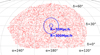 |
Fig. 1. Angular distribution of CMASS galaxies of the northern Galactic cap within a slice of 100 h−1 Mpc thickness centered at the redshift zcen = 0.52, shown in Mollweide equal-area projection in the equatorial coordinate system (α and δ denote right ascension and declination, respectively). In order to increase the visibility so that the distribution of galaxies is clear, only 14% of the total data points were randomly selected and displayed. For a comparison of spatial scales, two circles with radii of 70 and 300 h−1 Mpc have been added. |
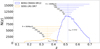 |
Fig. 2. Number distributions of the LRG and CMASS galaxies over redshift. The width of redshift in the histograms is Δz = 3.25 × 10⁻³. Also shown are the redshift ranges enclosed by spheres with a series of radii from 50 to 300 h−1 Mpc, centered at zcen = 0.35 for LRG and zcen = 0.52 for CMASS (denoted as vertical dotted lines). For radii of 250 and 300 h−1 Mpc in the case of the CMASS sample, the redshift ranges have been shifted to the higher redshift to include more galaxies within the range specified. |
Due to the mask of bright stars, centerposts of telescope, observation failure, and a number of various reasons, the galaxies within the BOSS survey region were not completely surveyed, and thus missing and incomplete regions exist. We reconstructed the completeness of the survey by combining the BOSS survey boundaries and a collection of mask information provided by the BOSS website1. The MANGLE software was used to interpret and combine the mask files with a polygon format (Hamilton & Tegmark 2004; Swanson et al. 2008). The final output of the MANGLE for the completeness of the CMASS sample was transformed into the Hierarchical Equal Area iso-Latitude Pixelization (HEALPix) format where the individual pixels cover equal area on the sky (Górski et al. 2005). The CMASS sector completeness within the BOSS survey region is shown in Fig. 3. Hereafter, we call this completeness map the angular selection function (ASF) of the CMASS sample.
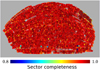 |
Fig. 3. Sector completeness map of the BOSS DR12 CMASS sample. The gray color indicates the outer region of the survey or no data. |
In our analysis, we take into account the fact that different weights are assigned to galaxies that were placed in various observation environments. For example, a galaxy is given more weight if the nearest neighbor of this galaxy is located within the diameter of the spectroscopic fiber and the redshift of the neighboring galaxy was not obtained due to fiber collision. We corrected for the effect of the fiber collision (wcp) and the redshift failure (wzf). Additionally, we also applied weights to account for the systematic relation between the number density of observed galaxies and stellar density (wstar) and seeing (wsee). Finally, each galaxy was assigned the combined weight defined as wtot = (wcp + wzf − 1)wstarwsee. By combining the survey completeness (wsc) at the angular position of a galaxy (Fig. 3) and the weights assigned to it, we obtained the contribution of each galaxy in the galaxy count as wtot/wsc.
3.1.2. Random catalogs
Before testing the homogeneity of matter distribution using the CMASS galaxies, first we needed to establish a clear criterion for determining homogeneity. Although homogeneity implies that the physical state is the same at all locations, in principle it is impossible for a finite number of points within a space to be homogeneously distributed. This is because fictitious clustering and a density inhomogeneity are always visible when a finite number of data points are generated even with uniform probability. Therefore, here we establish the criterion for homogeneity from a statistical point of view. The simplest way to do this is to use the distribution of random points following the Poisson distribution as the criterion for homogeneity. The finite number of points randomly distributed by the Poisson distribution shows fluctuations in the number density from place to place. On a small scale, the actual distribution of galaxies tends to show a larger fluctuation due to clustering of galaxies than expected in the Poisson distribution. Since these fluctuations are expected to decrease with increasing scale, we can determine the HS from which the distribution of galaxies begins to match the random distribution within a statistically acceptable range.
In this work, we have made one thousand random catalogs by considering the observational characteristics of the CMASS sample, each containing data points equal to the number of CMASS galaxies. The random data points were generated within the survey region using the radial number distribution and sector completeness as the probability density functions. However, the random data points were assigned a uniform weight (wtot = 1), unlike the galaxies with various weights. Thus, the contribution of each point to the count is 1/wsc for the random catalog. We analyzed these random catalogs in the same way as the CMASS sample is analyzed.
3.1.3. HR3 mock catalogs
To test the homogeneity of the CMASS galaxy distribution, in addition to the random distribution, we also analyzed the mock galaxy distribution expected in the standard cosmological model, and we compared the results with that of the actual galaxy distribution. Here we have produced the CMASS mock catalogs from the two model-derived data sets.
The first one we used is the 27 all-sky mock BOSS survey data provided by the Korea Institute of Advanced Study2. The data were derived from the HR3 simulation, which is one of the largest N-body simulations in volume to date with 72103 dark matter particles within the volume of (10.815 h−1 Gpc)3 (Kim et al. 2011). The halos were picked up as mock galaxies at redshift range 0.43 < z < 0.7 considering the redshift-dependent mass limit determined from the expected galaxy number density of the BOSS survey (see Sect. 4.2 of Kim et al. 2011). Figure 4 compares the radial number distributions of HR3 mock galaxies (extracted from one of the pieces of mock BOSS survey data) and the CMASS galaxies. For HR3 data, the mock galaxies corresponding to the percentage of CMASS sector completeness were randomly selected within the survey region. We would like to note that the radial number distribution of the selected HR3 mock galaxies is less than that of the CMASS sample at a redshift range of 0.47 < z < 0.55, and we excluded the CMASS galaxies that are fainter than an absolute magnitude of −20.2 in r-band and made the galaxy number density around z = 0.5 smaller than the HR3 data so that mock catalogs for the CMASS sample can be safely obtained. Within the CMASS survey region, considering the CMASS radial number distribution and angular selection function, we extracted massive halos with the same number of the magnitude-limited CMASS galaxies in decreasing order of halo mass. For each piece of mock SDSS-III survey data that covers the whole sky, it is possible to extract the four independent mock catalogs for the CMASS NGC region. Thus, we made a total of 108 independent mock catalogs. The limited number of mock catalogs makes it possible to judge the statistical significance only up to 2σ. Each HR3 mock catalog contains 395 011 data points. We also made separate sets of random catalogs that match the new radial number distribution of the magnitude-limited CMASS sample (see Fig. 4).
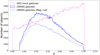 |
Fig. 4. Radial number distributions of HR3 mock galaxies (N = 920 421) from the first 27 lightcones (only ASF was applied), the CMASS galaxies (N = 568 776), and the CMASS galaxies brighter than the absolute magnitude of −20.2 in r-band (N = 395 011). |
Our method of generating mock catalogs has a limitation in that it cannot specifically mimic the process in which CMASS galaxies are selected by various color-cuts. However, our method is valid in that it mimics massive galaxies of the CMASS sample by preferentially choosing heavier halos, taking into account the known relation that a more massive halo contains a brighter galaxy (Kim et al. 2008).
3.1.4. Log-normal mock catalogs
The second piece of data pertains to the mock galaxies extracted from the log-normal simulations, which is an inexpensive way of generating realizations of nonlinear density fluctuations. We used a publicly available code to generate log-normal realizations of galaxies in redshift space3 (Agrawal et al. 2017). The code generates a log-normal matter density field from a matter power spectrum of the ΛCDM model, then it draws Poisson-distributed mock galaxies with a number expected by the log-normal density field at a given position in space. It has been confirmed whether the generated mock galaxies give two-point statistics similar to that of a standard ΛCDM model (Agrawal et al. 2017).
Using the flat ΛCDM model favored by the Planck 2018 TT, TE, EE+lowE+lensing data (Planck Collaboration VI 2020), we obtained the log-normal realizations of galaxies at redshift zcen = 0.52. Since galaxies in the log-normal realizations do not have mass information, there is a disadvantage that galaxies cannot be selected in order of mass as in the HR3 mock catalog. To obtain the statistics similar to CMASS galaxies, we assume the bias of galaxies relative to dark matter to be b = 2.2, which is a value adopted by the BOSS collaboration for generating mock catalogs (Alam et al. 2017). This value does not statistically deviate from the measurement of other studies (Guo et al. 2013; Nuza et al. 2013; Zhai et al. 2017). Finally, we generated one thousand mock catalogs by randomly selecting mock galaxies in the log-normal realizations considering the radial number distribution and sector completeness of the CMASS sample so that the generated log-normal galaxies follow the magnitude-limited CMASS galaxies. We also produced 1000 log-normal catalogs even assuming a lower bias of b = 1.8 as suggested in Rodríguez-Torres et al. (2016). It is shown that the log-normal catalogs with b = 1.8 do not provide statistics similar to the CMASS data (see Sect. 3.3.2 below). As in the random catalogs, we assigned uniform weights (wtot = 1) for all points in both the HR3 mock catalogs and the log-normal mock catalogs.
3.2. Method: Counting galaxies with truncated cones
To quantitatively test whether the three-dimensional spatial distribution of galaxies is homogeneous, we applied the galaxy counting method to the CMASS sample, random catalogs, and two mock catalogs. Hogg et al. (2005) and Ntelis et al. (2017) used the count-in-sphere method to judge whether the distribution of galaxies is homogeneous by comparing the number of galaxies within a sphere of a specific radius with that of the random distributions. On the other hand, Park et al. (2017) tested the homogeneity of the LRG distribution by counting galaxies within a truncated cone instead of the sphere. Unlike the count-in-sphere method which needs the three-dimensional spatial distribution of galaxies, the count-in-truncated-cone method with a fixed redshift center is less dependent on specific cosmological models in that galaxies are counted in the given redshift space, not in real space. In addition, counting galaxies within a truncated cone enables us to define a criterion for homogeneity without the need to consider different statistical weights given to galaxies that are unevenly distributed along the radial direction. This is because the accumulated statistical weight of the line-of-sight direction is the same no matter which direction we see within the truncated cone.
In this work, we use the count-in-truncated-cone method suggested by Park et al. (2017). We consider a 7 h−1 Mpc-thick slice for a central redshift zcen = 0.52, where CMASS galaxies are the most dense. There are 9770 CMASS galaxies in this slice. The thickness of the slice was chosen to control the number of galaxies (to be located at the center of the truncated cone) to an appropriate level of about 10 000. This number is suitable for closely looking at the direction-dependency of galaxy counts within the survey region and for performing calculations within a reasonable time. For each galaxy, we considered a sphere of comoving radius R that is centered at the slice, but at the galaxy’s angular position, and we constructed a truncated cone that is circumscribed about the sphere (Fig. 5). The apparent angular radius of the truncated cone seen from the observer is given by θR = sin−1(R/rcen), where rcen is the comoving distance to the center of the slice. The redshift z1 (z2) corresponding to the near (far) side of a truncated cone is transformed from the comoving distance rcen − R (rcen + R) in the fiducial ΛCDM model. For radii from 250 to 300 h−1 Mpc, however, the rcen − R becomes less than the distance to the minimum redshift (z = 0.43). Thus, in these cases, z1 was set to z = 0.43 and z2 was set to the higher value so that the interval z2 − z1 can span a range of 2R and include more galaxies within the range (see Fig. 2).
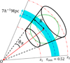 |
Fig. 5. Truncated cone circumscribed about a sphere of radius R. The apparent angular radius of the truncated cone (or the sphere) as seen from the observer at O is θR. Redshifts z1 and z2, the lower and upper limits of the truncated cone, respectively, vary as the radius of the sphere at the central redshift zcen varies. The thin slice at zcen has a thickness of Δr = 7 h−1 Mpc. We counted galaxies inside the truncated cone which is centered on every galaxy within the slice. |
Next, we calculated a statistical measure of homogeneity ξ, defined as the number density within the truncated cone divided by the number density within the slice covering the whole survey area from redshift z1 to z2,
 (1)
(1)
where Ntrc (Nslice) denotes the number of galaxies within the truncated cone (slice) and Vtrc (Vslice) is the volume of the truncated cone (slice). For a homogeneous distribution, the statistic ξ is expected to converge to one as the radius increases. However, when the radius is large enough to cover the entire survey region, this statistic has a characteristic of reaching one, in principle, even when the distribution considered is not homogeneous.
Due to the survey boundaries, masks, and holes, a truncated cone is not complete. The partial volume of the truncated cone was calculated by summing the volume elements corresponding to each HEALpix pixel in the pixelized area occupied by the truncated cone on the sky (see the Appendix in Park et al. 2017 for a detailed description). For a varying radius from R = 30 h−1 Mpc to 300 h−1 Mpc with steps of 10 h−1 Mpc (totally 28 steps), we calculated ξ and the volume of the partial truncated cone for every galaxy within the slice with z = zcen and a 7 h−1 Mpc width. The maximum radius of 300 h−1 Mpc is limited by the depth of the CMASS sample, that is about 600 h−1 Mpc.
Given the individual measurements of ξ for every galaxy within the slice, we calculated the mean (⟨ξ⟩), standard deviation (σξ), skewness (skewξ), and kurtosis (kurtξ) of the measured ξs. During the calculation of these statistics, we assigned each measured ξ a statistical weight by the volume of the partial truncated cone. Thus, the ξs measured near the survey boundary usually have lower statistical weights than those near the center of the survey region. For each radius scale, these statistics are compared with those estimated from the random and mock catalogs. The significant deviation of the measured value from the expectation of the random or mock distributions may imply a deviation from the homogeneity or the present cosmological model.
3.3. Results
3.3.1. Comparison with random data
As the homogeneous distribution, we used the random Poisson distribution. Comparisons are made in Figs. 6a,b, which show the mean (⟨ξ⟩) and the standard deviation (σξ) of ξs calculated from the unmodified CMASS sample and the corresponding 1000 random catalogs. We can see that ⟨ξ⟩s from both the CMASS sample and random data approach one as the radius increases. However, unlike the random distributions, the ⟨ξ⟩ of the CMASS sample does not fully converge to one, but it shows a large deviation, which is maintained even at the largest radius. The σξ also significantly deviates from the expected range of the random distributions. For ⟨ξ⟩, the deviations are 61σ at 70 h−1 Mpc and 5.5σ at 300 h−1 Mpc; and for σξ, the deviations are 93σ at 70 h−1 Mpc and 34σ at 300 h−1 Mpc (see Fig. 7). The deviations in the mean and standard deviation show that CMASS galaxies are far from the random distributions even at the largest scale. On the other hand, the skewness and kurtosis of ξ statistics presented in Fig. 8 show no significant anomaly of the CMASS sample compared with the random data. Also shown are the trends in the magnitude-limited CMASS sample and random data, where deviations from the random data are far more significant than the original ones.
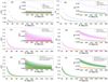 |
Fig. 6. Mean (⟨ξ⟩) and standard deviation (σξ) of ξ as a function of radius (R). The top panels (a,b) show the results of the unmodified CMASS sample (blue dots) and the corresponding 1000 random catalogs (cyan dots), together with those of the magnitude-limited CMASS sample (blue plus signs) and the corresponding 1000 random catalogs (brown dots). The results of the 108 HR3 mock catalogs (pink dots) are shown in the middle panels (c,d), together with those of the magnitude-limited CMASS sample and the corresponding random catalogs. The bottom panels (e,f) present the results of the log-normal mock catalogs generated with a bias factor b = 2.2 (green dots). For a comparison, the results for b = 1.8 are shown as cross marks (×s). The shaded regions in each panel, in order from dark to light, represent 1, 2, and 3 sigma confidence regions, which have been estimated from measured means and standard deviations of individual random or mock catalogs. The information of the shaded regions between the specified radius scales are interpolated. |
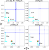 |
Fig. 7. Mean and standard deviation diagrams of the unmodified CMASS sample (blue markers and solid lines) and the corresponding 1000 random catalogs (cyan dots and histograms) for four different radii at the central redshift zcen = 0.52. Results of the magnitude-limited CMASS sample (faint blue markers and dotted lines) and the corresponding 108 random catalogs (brown markers) are also shown for comparison. The deviations of the CMASS sample from the 1000 random data are indicated in units of standard deviation (σ). |
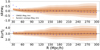 |
Fig. 8. Skewness (skewξ; top) and kurtosis (kurtξ; bottom) of ξ as a function of radius (R). The result of the magnitude-limited CMASS sample (blue dots) is compared with the average and 1–3σ confidence regions of the 108 random catalogs. |
3.3.2. Comparison with two mock catalogs
Figures 6c,d and 6e,f compare ⟨ξ⟩ and σξ variations of the CMASS sample with those of HR3 and log-normal mock catalogs, respectively. Here, the magnitude-limited CMASS sample and the corresponding random catalogs have been used. For both ⟨ξ⟩ and σξ, the CMASS sample relatively agrees well with both mock samples (see Fig. 9 for HR3 mock samples). We note that the log-normal galaxies generated with a lower value of bias factor (b = 1.8) have lower amplitudes for the mean and standard deviation of the ξ statistic. Thus, the CMASS galaxies are distributed as expected from a theoretically estimated distribution.
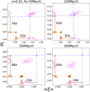 |
Fig. 9. Same as Fig. 7, but for the magnitude-limited CMASS sample, 108 HR3 mock catalogs (pink dots and histograms), and the corresponding 108 random catalogs (brown dots and histograms). |
For ⟨ξ⟩, although the values of mock catalogs tend to approach the result of the random distribution as the scale increases, the ⟨ξ⟩ of the CMASS sample tends to stay constant starting from 230 h−1 Mpc. This anomaly can be explained by the presence of peculiar overdense regions in the CMASS sample. If there are noticeable overdense regions with more clustering within the survey volume, naturally ⟨ξ⟩ is expected to be greater than one. Although not a major effect, it should also be taken into account that galaxies located near the CMASS boundary contribute less to ⟨ξ⟩ because in this case only the partial volume of the truncated cone is used as weight. The constant behavior of ⟨ξ⟩ at large scales with a significant deviation from unity can also be found in the mock catalogs. Figure 10 shows the behavior of ⟨ξ⟩ as a function of the radius scale for the cases of the maximum and minimum ⟨ξ⟩ at R = 300 h−1 Mpc among the 1000 log-normal mock catalogs. Figure 11 compares the distributions of ξ on the CMASS survey region for the magnitude-limited CMASS sample, a (magnitude-limited) random catalog, and two log-normal mock catalogs that show the maximum or minimum values of ⟨ξ⟩ at a 300 h−1 Mpc scale (see Sect. 3.4 for a detailed description of how to produce these maps). In the ξ distribution of the CMASS sample, it is seen that an overdense area exists in the central part of the survey region. In the case of the mock catalog showing the maximum ⟨ξ⟩ value, the overall distribution is similar. On the other hand, for the mock catalog with the minimum ⟨ξ⟩, it appears that there are relatively few overdense areas in the inner survey region.
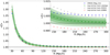 |
Fig. 10. Variation of ⟨ξ⟩ as a function of radius R for log-normal mock catalogs (green dots with shaded regions) and the magnitude-limited CMASS sample (blue dots), which is the same as in Fig. 6e. Here the cases of the maximum (black plus signs) and the minimum (red cross marks) ⟨ξ⟩ at 300 h−1 Mpc among the 1000 log-normal mock catalogs have been added. |
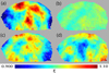 |
Fig. 11. Maps showing ξ distributions on the CMASS survey region, estimated from the magnitude-limited CMASS sample (a), a (magnitude-limited) random catalog (b), and two log-normal catalogs with the maximum (c) and minimum (d) values of ⟨ξ⟩ at R = 300 h−1 Mpc scale. |
In σξ, both kinds of mock samples significantly deviate from the random data, and the deviation becomes even larger for the CMASS galaxies at the largest scale (see Figs. 6d,f, and 7). As is shown in Fig. 9, the deviations of the magnitude-limited CMASS galaxies from the random expectations are 19σ for ⟨ξ⟩ and 40σ for σξ at R = 300 h−1 Mpc. We note that the CMASS galaxies show similar ⟨ξ⟩ and σξ as mock galaxies on small scales, but the difference between the two becomes more significant as the scale increases. At the largest scale, the CMASS sample tends to deviate by 3σ or more from the mock samples. Further investigation is needed to explain this discrepancy.
3.3.3. Comparison with theoretical power spectrum
In the previous subsection, we have compared the distribution of the CMASS galaxies with those in two theoretical mock catalogs. The distribution of galaxies in the mock catalogs contains information of the nonlinear mass fluctuations. Here we investigate whether the linear matter density fluctuations, which are the result of the primordial fluctuations developed by the linear perturbation theory, can explain the CMASS result without taking the effects of nonlinear gravitational evolution into account. For this, we compared our estimation of σξ of the CMASS sample with the theoretically estimated amplitude of mass fluctuations. The variance of mass fluctuations expected within a sphere of radius R is given by Peebles (1993)
 (2)
(2)
where P(k) denotes the matter power spectrum at wavenumber k, and WR(k) is the Fourier transformation of a spherical top-hat window function that assigns 3/(4πR3) inside the sphere and 0 otherwise and is written as
![Mathematical equation: $$ \begin{aligned} W_R(\mathbf k )=\frac{3}{(kR)^3} \left[\sin (kR)-kR\cos (kR) \right]. \end{aligned} $$](/articles/aa/full_html/2022/04/aa41909-21/aa41909-21-eq3.gif) (3)
(3)
Figure 12 compares the theoretical prediction of matter density fluctuations σ(R) at various scales with the measured deviation of galaxy number density σξ of the CMASS sample and two mock catalogs. In our calculation, we used the code for anisotropies in the microwave background (CAMB; Lewis & Challinor 2011) to obtain the linear matter power spectrum at z = 0.52 in a flat ΛCDM cosmological model that best fits the Planck 2018 TT, TE, EE+lowE data (Planck Collaboration VI 2020). The σ(R) shown in Fig. 12 was obtained by inserting the linear power spectrum into Eq. (2) and multiplying with the bias factor b = 2.2, which is consistent with the values estimated in the previous studies (Guo et al. 2013; Nuza et al. 2013; Zhai et al. 2017). The σ(R) obtained in this way is in good agreement with σξ(R) of both HR3 and log-normal mock catalogs at all scales above 50 h−1 Mpc.
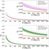 |
Fig. 12. Comparison of σξ of the CMASS sample and the HR3 and log-normal mock catalogs (same as Figs. 6d,f), together with the mass fluctuations σ(R) of linear density fields expected in the standard ΛCDM model (Planck Collaboration VI 2020). |
3.4. Cosmic landscape
The count-in-truncated cone method used here to test the homogeneity of the galaxy distribution is also useful for visualizing the results and making intuitive comparisons. Figure 13 visualizes the clustered nature of the CMASS galaxies compared to a random realization. Whereas our statistical studies were based on galaxy-centered counting, the results shown here are based on the pixel-centered counting. We divided the survey area into about 132 000 pixels using the HEALpix program with a resolution parameter as Nside = 256 (Górski et al. 2005). Then, we placed a truncated cone in the center of every pixel and calculated ξ. Figure 13 is the ξ distribution maps and directly shows how the averaged-over-the-radius density changes with position. To compare this with the CMASS sample, just one random catalog is selected out of the 1000 catalogs.
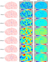 |
Fig. 13. Cosmic landscape in galaxy number count. Left panel: CMASS galaxies within a thin slice at the central redshift zcen. Circles of different sizes of radius (R = 50, 70, 100, 150, 200, 250, 300 h−1 Mpc) are shown together. The redshift ranges are presented in Fig. 2. Middle and right panels: maps of ξ estimated from the unmodified CMASS sample (left) and a random catalog (right panel). |
Figure 13 shows that the CMASS galaxies are far more clustered than the random distribution in all scales, and Table 1 compares the density extremum (maximum and minimum) between the CMASS sample and the random data. For the often claimed HS, 70 h−1 Mpc, the density maximum of the CMASS sample is 79% higher than the mean, while for the random one, it is only 18%; the ratio between the maximum and minimum is 3.30 for the CMASS sample, while it is only 1.39 for the random data. It is not easy to call a distribution with such large fluctuations homogeneous. Even at 300 h−1 Mpc, it is difficult to say that the distribution of galaxies is homogeneous: ξs at maximum for the CMASS and random data are 10% and 2% higher than mean, respectively, and the ratio between the maximum and minimum is 1.20 versus 1.05.
3.5. Conclusion of the test
In this section, we have studied the inhomogeneous nature of galaxy distribution using the BOSS CMASS DR12 sample, which includes 932 517 galaxies within the redshift range between 0.43 and 0.7 (Alam et al. 2015). We used the number count within truncated cones centered at every galaxy located at a narrow region around redshift 0.52. As the criterion of homogeneity, we statistically compared the observed distribution with the 1000 realizations of random Poisson distributions. Statistical comparisons were also carried out with two mock catalogs derived from theory: (i) 108 mock galaxy catalogs from the HR3 N-body numerical simulation (Kim et al. 2011) and (ii) the mock catalogs based on the log-normal distribution of matter density (Agrawal et al. 2017). We also compared σ(R) estimated from the linear matter power spectrum.
The result shows that the difference between the CMASS sample and the random data reduces as the scale becomes larger (see Figs. 6a,b, and 8). However, even in the largest statistically meaningful scale, that is the radius around 300 h−1 Mpc, the difference is still significant. Even at the largest scale, the deviation of the CMASS sample from the Poisson distribution is around 34σ to 40σ in standard deviation (σξ) and around 5σ to 19σ in the mean (⟨ξ⟩) (see Figs. 7 and 9). Thus, even on this largest available scale, it is impossible for the CMASS data to appear in random realizations. The cosmic landscape shown in Fig. 13 visually confirms our conclusion. The CMASS galaxies are far more clustered than the randomly distributed points in all currently available scales.
However, our comparison of the CMASS sample with the two mock catalogs shows consistency between the observation (CMASS sample) and theory (two mock catalogs; see Figs. 6c,f, 9, and 12). A statistical anomaly in ⟨ξ⟩ identified at a large scale is explained by the presence of overdense regions located in the CMASS survey area. We confirmed that the same phenomenon occurs in the log-normal mock catalogs with similar overdensities (see Sect. 3.3 and Figs. 10 and 11). A statistical anomaly in σξ compared with the two pieces of mock data identified at a large scale in Figs. 6d,f, and 9 needs further study.
Therefore, we conclude that while the observation is consistent with the current paradigm of modern cosmology, the CP is not in the currently available galaxy distribution sample and nor is it demanded by theory. A clear resolution of this seemingly contradictory conclusion is made in Sects. 2 and 4.
4. Discussion
Einstein’s gravity directly connects the matter with the spacetime curvature. However, the CP is implemented in the metric. As the curvature is a quadratic derivative of the metric, the near-homogeneity in the metric does not demand similar near-homogeneity in the matter distribution. Such a difference is indeed the case in modern cosmology, especially on the far subhorizon scale. Our study in Sect. 3 confirms that matter distribution is far more inhomogeneous compared with the random Poisson distribution, which is our criterion for the homogeneity. At the same time, we show that the matter distribution is consistent with theoretical predictions based on the simulation and power spectrum. Thus, the CP is not in the observed galaxy distribution, nor is it expected in theory.
We conclude that it is inadequate to search for the HS or the CP in the observed light or the matter distribution. As we show in Sect. 2, the CP is perfectly fine and well in the metric, a theoretical construct. However, this conclusion is valid under a subtle condition. Based on the Robertson-Walker metric as the background, we have shown that the deviations in metric are extremely small in the observed cosmic scale. Thus, our test implies that the CP is valid in modern cosmology if we assume that the CP is in the background. That is, ours is only a consistency test, not proof. Whether we can accept such a background geometry is an entirely different question that may demand another strategy. Until we resolve this aspect, the CP remains an assumption.
A proper answer to this question may require studying alternative models based on something other than Einstein’s CP. The CMB strongly supports the isotropy around us. Thus, one interesting possibility is constraining the spherically symmetric model based on Lemaître’s CP. After all, due to the nature of our observation, systematically observing past events as we observe further away, even under Einstein’s CP properly unfolded in the Universe, the observations are destined to be spherically symmetric with us at the center. The temporal evolution of cosmic structures and the observational difficulties increasing with distance would make the observation look spherically symmetric in any case. Constraining the spherically symmetric world models with us near the center is an important issue in this regard.
One consequence of our clarification, separating matter from the metric, is freeing our concept of the universe from dull homogeneity in its matter content on a large-scale because the CP in modern cosmology mainly concerns the metric only. Through the light, one may discover more diverse phenomena that may have distinct characteristics and may await new classification. Perhaps, if we may, “there are more things in the sky than are dreamt of in our theory.”
Although we have not found the HS in the currently available galaxy survey, this does not preclude its future discovery in a more in-depth survey. In modern cosmology, with δΦ/c2 ∼ (ℓ/ℓH)2δ, as the scale approaches the horizon scale, we should have δ ∼ δΦ/c2, thus the matter fluctuation (δ) becomes extremely small similar to the metric fluctuation. In this way, the Friedmann background world model should be recovered with the CP that is valid in both metric and matter in near-horizon scale structures. No such confirmation has been made yet. We anticipate practical difficulty as the scale approaches the horizon scale; the observed space (light cone) significantly deviates from the homogeneous space on which the CP is imposed. Still, although not relevant to the CP’s validity, the homogeneity test for matter should be continued using more extensive galaxy survey data, which will be undoubtedly available soon in the future.
Now, with the extreme level homogeneity in the cosmic metric being known, an important theoretical issue arises concerning its origin. Inflation provides an isotropization mechanism for homogeneous but anisotropic cosmologies (Wald 1983), but how about homogeneity? Why do we live in a universe with such extreme homogeneity in the metric? This is a mystery that has yet to be resolved. The anthropic principle is not an answer we anticipate as it merely claims the case as it happens to be.
The SDSS Science Archive Server, https://data.sdss.org/sas/dr12/boss/lss/geometry/
Available at http://sdss.kias.re.kr/astro/Horizon-Runs/Horizon-Run23.php
Acknowledgments
We wish to thank an anonymous referee for valuable comments and suggestions which help improve the manuscript. We thank Professors Donghui Jeong and Juhan Kim for useful discussion and suggestions. C.-G.P. was supported by the National Research Foundation of Korea (NRF) grant funded by the Korea government (MSIT) (No. 2020R1F1A1069250). H.N. was supported by the National Research Foundation of Korea funded by the Korean Government (No. 2018R1A2B6002466 and No. 2021R1F1A1045515). J.H. was supported by IBS under the project code IBSR018-D1 and by Basic Science Research Program through the National Research Foundation (NRF) of Korea funded by the Ministry of Science, ICT and Future Planning (No. 2018R1A6A1A06024970 and NRF-2019R1A2C1003031).
References
- Abazajian, K. N., Adelman-McCarthy, J. K., Agüeros, M. A., et al. 2009, ApJS, 182, 543 [Google Scholar]
- Agrawal, A., Makiya, R., Chiang, C.-T., et al. 2017, J. Cosmol. Astropart. Phys., 2017, 003 [CrossRef] [Google Scholar]
- Alam, S., Albareti, F. D., Allen de Prieto, C., et al. 2015, ApJS, 219, 12 [NASA ADS] [CrossRef] [Google Scholar]
- Alam, S., Atà, M., Bailey, S., et al. 2017, MNRAS, 470, 2617 [NASA ADS] [CrossRef] [Google Scholar]
- Anderson, L., Aubourg, E., Bailey, S., et al. 2012, MNRAS, 427, 3435 [Google Scholar]
- Angulo, R. E., Springel, V., White, S. D. M., et al. 2012, MNRAS, 426, 2046 [NASA ADS] [CrossRef] [Google Scholar]
- Bagla, J. S., Yadav, J., & Seshadri, T. R. 2008, MNRAS, 390, 829 [NASA ADS] [CrossRef] [Google Scholar]
- Dawson, K. S., Schlegel, D. J., Ahn, C. P., et al. 2013, AJ, 145, 10 [Google Scholar]
- Einstein, A. 1917a, Sitzungsberichte der Königlich Preußischen Akademie der Wissenschaften (Berlin: Seite), 142 [Google Scholar]
- Einstein, A. 1917b, in The Collected Papers of Albert Einstein, eds. R. Schulmann, A. J. Kox, M. Janssen, et al. (Princeton: Princeton University Press), Volume 8: The Berlin Years: Correspondence, 1914–1918 [Google Scholar]
- Eisenstein, D. J., Annis, J., Gunn, J. E., et al. 2001, AJ, 122, 2267 [Google Scholar]
- Eisenstein, D. J., Weinberg, D. H., Agol, E., et al. 2011, AJ, 142, 72 [Google Scholar]
- Ellis, G. F. R., Maartens, R., & MacCallum, M. A. H. 2012, Relativistic Cosmology (Cambridge: Cambridge University Press) [CrossRef] [Google Scholar]
- Friedmann, A. 1922, Z. Phys., 10, 377 [NASA ADS] [CrossRef] [Google Scholar]
- Friedmann, A. 1924, Z. Phys., 21, 326 [NASA ADS] [CrossRef] [Google Scholar]
- Górski, K. M., Hivon, E., Banday, A. J., et al. 2005, ApJ, 622, 759 [Google Scholar]
- Gott, J. R., Jurić, M., Schlegel, D., et al. 2005, ApJ, 624, 463 [NASA ADS] [CrossRef] [Google Scholar]
- Guo, H., Zehavi, I., Zheng, Z., et al. 2013, ApJ, 767, 122 [NASA ADS] [CrossRef] [Google Scholar]
- Habib, S., Pope, A., Finkel, H., et al. 2016, New Astron., 42, 49 [NASA ADS] [CrossRef] [Google Scholar]
- Hamilton, A. J. S., & Tegmark, M. 2004, MNRAS, 349, 115 [NASA ADS] [CrossRef] [Google Scholar]
- Heitmann, K., Frontiere, N., Sewell, C., et al. 2015, ApJS, 219, 34 [NASA ADS] [CrossRef] [Google Scholar]
- Hogg, D. W., Eisenstein, D. J., Blanton, M. R., et al. 2005, ApJ, 624, 54 [NASA ADS] [CrossRef] [Google Scholar]
- Hwang, J.-C., & Noh, H. 2006, MNRAS, 367, 1515 [NASA ADS] [CrossRef] [Google Scholar]
- Hwang, J.-C., & Noh, H. 2013, MNRAS, 433, 3472 [NASA ADS] [CrossRef] [Google Scholar]
- Hwang, J.-C., Noh, H., & Puetzfeld, D. 2008, J. Cosmol. Astropart. Phys., 03, 010 [CrossRef] [Google Scholar]
- Jeong, D., Gong, J.-O., Noh, H., & Hwang, J.-C. 2011, ApJ, 727, 22 [NASA ADS] [CrossRef] [Google Scholar]
- Kazin, E. A., Blanton, M. R., Scoccimarro, R., et al. 2010, ApJ, 710, 1444 [NASA ADS] [CrossRef] [Google Scholar]
- Kim, J., Park, C., & Choi, Y.-Y. 2008, ApJ, 683, 123 [NASA ADS] [CrossRef] [Google Scholar]
- Kim, J., Park, C., Gott, J. R., & Dubinski, J. 2009, ApJ, 701, 1547 [NASA ADS] [CrossRef] [Google Scholar]
- Kim, J., Park, C., Rossi, G., Lee, S. M., & Gott, J. R. 2011, J. Korean Astron. Soc., 44, 217 [NASA ADS] [CrossRef] [Google Scholar]
- Kim, J., Park, C., L’Huillier, B., & Hong, S. E. 2015, J. Korean Astron. Soc., 48, 213 [Google Scholar]
- Krasinski, A. 1997, Inhomogeneous Cosmological Models (Cambridge: Cambridge University Press) [CrossRef] [Google Scholar]
- Laurent, P. 2016, J. Cosmol. Astropart. Phys., 11, 060 [CrossRef] [Google Scholar]
- Lemaître, G. 1933, Annales de la Société Scientifique de Bruxelles, 53, 51 [NASA ADS] [Google Scholar]
- Lewis, A., & Challinor, A. 2011, Astrophysics Source Code Library [record ascl:1102.026] [Google Scholar]
- Lifshitz, E. M. 1946, J. Phys. (USSR), 10, 116 [Google Scholar]
- McCrea, W. H., & Milne, E. A. 1934, Quart. J. Math., os-5, 73 [CrossRef] [Google Scholar]
- Milne, E. A. 1934, Quart. J. Math., os-5, 64 [NASA ADS] [CrossRef] [Google Scholar]
- Ntelis, P., Hamilton, J.-C., Le Goff, J.-M., et al. 2017, J. Cosmol. Astropart. Phys., 06, 019 [CrossRef] [Google Scholar]
- Nuza, S. E., Sànchez, A. G., Prada, F., et al. 2013, MNRAS, 432, 743 [NASA ADS] [CrossRef] [Google Scholar]
- Park, C., Choi, Y.-Y., Kim, J., et al. 2012, ApJ, 759, L7 [Google Scholar]
- Park, C.-G., Hyun, H., Noh, H., & Hwang, J.-C. 2017, MNRAS, 469, 1924 [NASA ADS] [CrossRef] [Google Scholar]
- Peebles, P. J. E. 1993, Principles of Physical Cosmology (Princeton: Princeton University Press) [Google Scholar]
- Planck Collaboration I. 2014, A&A, 571, A1 [NASA ADS] [CrossRef] [EDP Sciences] [Google Scholar]
- Planck Collaboration VI. 2020, A&A, 641, A6 [NASA ADS] [CrossRef] [EDP Sciences] [Google Scholar]
- Potter, D., Stadel, J., & Teyssier, R. 2017, Comput. Astrophys. Cosmol., 4, 2 [NASA ADS] [CrossRef] [Google Scholar]
- Prada, F., Klypin, A. A., Cuesta, A. J., Betancort-Rijo, J. E., & Primack, J. 2012, MNRAS, 423, 3018 [NASA ADS] [CrossRef] [Google Scholar]
- Rodríguez-Torres, S. A., Chuang, C.-H., Prada, F., et al. 2016, MNRAS, 460, 1173 [CrossRef] [Google Scholar]
- Sarkar, P., Yadav, J., Pandey, B., & Bharadwaj, S. 2009, MNRAS, 399, L128 [NASA ADS] [CrossRef] [Google Scholar]
- Scrimgeour, M. I., Davis, T., Blake, C., et al. 2012, MNRAS, 425, 116 [NASA ADS] [CrossRef] [Google Scholar]
- Shibata, M., & Asada, H. 1995, Progr. Theoret. Phys., 94, 11 [NASA ADS] [CrossRef] [Google Scholar]
- Smoot, G. F., Bennett, C. L., Kogut, A., et al. 1992, ApJ, 396, L1 [Google Scholar]
- Spergel, D. N., Verde, L., Peiris, H. V., et al. 2003, ApJS, 148, 175 [Google Scholar]
- Springel, V., White, S. D. M., Jenkins, A., et al. 2005, Nature, 435, 629 [Google Scholar]
- Swanson, M. E. C., Tegmark, M., Hamilton, A. J. S., & Hill, J. C. 2008, MNRAS, 387, 1391 [NASA ADS] [CrossRef] [Google Scholar]
- Sylos Labini, F. 2011, J. Cosmol. Astropart. Phys., 15, 6110 [Google Scholar]
- Sylos Labini, F., & Baryshev, Y. V. 2010, J. Cosmol. Astropart. Phys., 06, 021 [CrossRef] [Google Scholar]
- Sylos Labini, F., Vasilyev, N. L., Pietronero, L., & Baryshev, Y. V. 2009, EPL, 86, 49001 [NASA ADS] [CrossRef] [EDP Sciences] [Google Scholar]
- Teyssier, R., Pires, S., Prunet, S., et al. 2009, A&A, 497, 335 [NASA ADS] [CrossRef] [EDP Sciences] [Google Scholar]
- Vogelsberger, M., Marinacci, F., Torrey, P., & Puchwein, E. 2020, Nat. Rev. Phys, 2, 42 [NASA ADS] [CrossRef] [Google Scholar]
- Wald, R. M. 1983, Phys. Rev. D, 28, 2118 [NASA ADS] [CrossRef] [Google Scholar]
- Yadav, J., Bharadwaj, S., Pandey, B., & Seshadri, T. R. 2005, MNRAS, 364, 601 [NASA ADS] [CrossRef] [Google Scholar]
- Yadav, J. K., Bagla, J. S., & Khandai, N. 2010, MNRAS, 405, 2009 [NASA ADS] [Google Scholar]
- Zhai, Z., Tinker, J. L., Hahn, C., et al. 2017, ApJ, 848, 76 [NASA ADS] [CrossRef] [Google Scholar]
All Tables
All Figures
|
Fig. 1. Angular distribution of CMASS galaxies of the northern Galactic cap within a slice of 100 h−1 Mpc thickness centered at the redshift zcen = 0.52, shown in Mollweide equal-area projection in the equatorial coordinate system (α and δ denote right ascension and declination, respectively). In order to increase the visibility so that the distribution of galaxies is clear, only 14% of the total data points were randomly selected and displayed. For a comparison of spatial scales, two circles with radii of 70 and 300 h−1 Mpc have been added. |
| In the text | |
|
Fig. 2. Number distributions of the LRG and CMASS galaxies over redshift. The width of redshift in the histograms is Δz = 3.25 × 10⁻³. Also shown are the redshift ranges enclosed by spheres with a series of radii from 50 to 300 h−1 Mpc, centered at zcen = 0.35 for LRG and zcen = 0.52 for CMASS (denoted as vertical dotted lines). For radii of 250 and 300 h−1 Mpc in the case of the CMASS sample, the redshift ranges have been shifted to the higher redshift to include more galaxies within the range specified. |
| In the text | |
|
Fig. 3. Sector completeness map of the BOSS DR12 CMASS sample. The gray color indicates the outer region of the survey or no data. |
| In the text | |
|
Fig. 4. Radial number distributions of HR3 mock galaxies (N = 920 421) from the first 27 lightcones (only ASF was applied), the CMASS galaxies (N = 568 776), and the CMASS galaxies brighter than the absolute magnitude of −20.2 in r-band (N = 395 011). |
| In the text | |
|
Fig. 5. Truncated cone circumscribed about a sphere of radius R. The apparent angular radius of the truncated cone (or the sphere) as seen from the observer at O is θR. Redshifts z1 and z2, the lower and upper limits of the truncated cone, respectively, vary as the radius of the sphere at the central redshift zcen varies. The thin slice at zcen has a thickness of Δr = 7 h−1 Mpc. We counted galaxies inside the truncated cone which is centered on every galaxy within the slice. |
| In the text | |
|
Fig. 6. Mean (⟨ξ⟩) and standard deviation (σξ) of ξ as a function of radius (R). The top panels (a,b) show the results of the unmodified CMASS sample (blue dots) and the corresponding 1000 random catalogs (cyan dots), together with those of the magnitude-limited CMASS sample (blue plus signs) and the corresponding 1000 random catalogs (brown dots). The results of the 108 HR3 mock catalogs (pink dots) are shown in the middle panels (c,d), together with those of the magnitude-limited CMASS sample and the corresponding random catalogs. The bottom panels (e,f) present the results of the log-normal mock catalogs generated with a bias factor b = 2.2 (green dots). For a comparison, the results for b = 1.8 are shown as cross marks (×s). The shaded regions in each panel, in order from dark to light, represent 1, 2, and 3 sigma confidence regions, which have been estimated from measured means and standard deviations of individual random or mock catalogs. The information of the shaded regions between the specified radius scales are interpolated. |
| In the text | |
|
Fig. 7. Mean and standard deviation diagrams of the unmodified CMASS sample (blue markers and solid lines) and the corresponding 1000 random catalogs (cyan dots and histograms) for four different radii at the central redshift zcen = 0.52. Results of the magnitude-limited CMASS sample (faint blue markers and dotted lines) and the corresponding 108 random catalogs (brown markers) are also shown for comparison. The deviations of the CMASS sample from the 1000 random data are indicated in units of standard deviation (σ). |
| In the text | |
|
Fig. 8. Skewness (skewξ; top) and kurtosis (kurtξ; bottom) of ξ as a function of radius (R). The result of the magnitude-limited CMASS sample (blue dots) is compared with the average and 1–3σ confidence regions of the 108 random catalogs. |
| In the text | |
|
Fig. 9. Same as Fig. 7, but for the magnitude-limited CMASS sample, 108 HR3 mock catalogs (pink dots and histograms), and the corresponding 108 random catalogs (brown dots and histograms). |
| In the text | |
|
Fig. 10. Variation of ⟨ξ⟩ as a function of radius R for log-normal mock catalogs (green dots with shaded regions) and the magnitude-limited CMASS sample (blue dots), which is the same as in Fig. 6e. Here the cases of the maximum (black plus signs) and the minimum (red cross marks) ⟨ξ⟩ at 300 h−1 Mpc among the 1000 log-normal mock catalogs have been added. |
| In the text | |
|
Fig. 11. Maps showing ξ distributions on the CMASS survey region, estimated from the magnitude-limited CMASS sample (a), a (magnitude-limited) random catalog (b), and two log-normal catalogs with the maximum (c) and minimum (d) values of ⟨ξ⟩ at R = 300 h−1 Mpc scale. |
| In the text | |
|
Fig. 12. Comparison of σξ of the CMASS sample and the HR3 and log-normal mock catalogs (same as Figs. 6d,f), together with the mass fluctuations σ(R) of linear density fields expected in the standard ΛCDM model (Planck Collaboration VI 2020). |
| In the text | |
|
Fig. 13. Cosmic landscape in galaxy number count. Left panel: CMASS galaxies within a thin slice at the central redshift zcen. Circles of different sizes of radius (R = 50, 70, 100, 150, 200, 250, 300 h−1 Mpc) are shown together. The redshift ranges are presented in Fig. 2. Middle and right panels: maps of ξ estimated from the unmodified CMASS sample (left) and a random catalog (right panel). |
| In the text | |
Current usage metrics show cumulative count of Article Views (full-text article views including HTML views, PDF and ePub downloads, according to the available data) and Abstracts Views on Vision4Press platform.
Data correspond to usage on the plateform after 2015. The current usage metrics is available 48-96 hours after online publication and is updated daily on week days.
Initial download of the metrics may take a while.