| Issue |
A&A
Volume 660, April 2022
|
|
|---|---|---|
| Article Number | A37 | |
| Number of page(s) | 15 | |
| Section | The Sun and the Heliosphere | |
| DOI | https://doi.org/10.1051/0004-6361/202140877 | |
| Published online | 06 April 2022 | |
DeSIRe: Departure coefficient aided Stokes Inversion based on Response functions
1
Instituto de Astrofísica de Canarias, 38200 La Laguna, Tenerife, Spain
e-mail: This email address is being protected from spambots. You need JavaScript enabled to view it.
2
Departamento de Astrofísica, Univ. de La Laguna, La Laguna, Tenerife 38205, Spain
3
Rosseland Centre for Solar Physics, University of Oslo, PO Box 1029, Blindern, 0315 Oslo, Norway
4
Institute of Theoretical Astrophysics, University of Oslo, PO Box 1029, Blindern, 0315 Oslo, Norway
5
Institute of Space and Astronautical Science, Japan Aerospace Exploration Agency, Sagamihara, Kanagawa 252-5210, Japan
6
Univ Coimbra, IA, CITEUC, OGAUC, Coimbra, Portugal
7
National Solar Observatory, University of Colorado Boulder, 3665 Discovery Drive, Boulder, CO 80303, USA
8
Instituto de Astrofísica de Andalucía (CSIC), Apdo. de Correos 3004, 18080 Granada, Spain
Received:
25
March
2021
Accepted:
28
January
2022
Abstract
Future ground-based telescopes, such as the 4-metre class facilities DKIST and EST, will dramatically improve on current capabilities for simultaneous multi-line polarimetric observations in a wide range of wavelength bands, from the near-ultraviolet to the near-infrared. As a result, there will be an increasing demand for fast diagnostic tools, i.e., inversion codes, that can infer the physical properties of the solar atmosphere from the vast amount of data these observatories will produce. The advent of substantially larger apertures, with the concomitant increase in polarimetric sensitivity, will drive an increased interest in observing chromospheric spectral lines. Accordingly, pertinent inversion codes will need to take account of line formation under general non-local thermodynamic equilibrium (NLTE) conditions. Several currently available codes can already accomplish this, but they have a common practical limitation that impairs the speed at which they can invert polarised spectra, namely that they employ numerical evaluation of the so-called response functions to changes in the atmospheric parameters, which makes them less suitable for the analysis of very large data volumes. Here we present DeSIRe (Departure coefficient aided Stokes Inversion based on Response functions), an inversion code that integrates the well-known inversion code SIR with the NLTE radiative transfer solver RH. The DeSIRe runtime benefits from employing analytical response functions computed in local thermodynamic equilibrium (through SIR), modified with fixed departure coefficients to incorporate NLTE effects in chromospheric spectral lines. This publication describes the operating fundamentals of DeSIRe and describes its behaviour, robustness, stability, and speed. The code is ready to be used by the solar community and is being made publicly available.
Key words: Sun: magnetic fields / techniques: polarimetric / atomic data / radiative transfer
© ESO 2022
1. Introduction
Our knowledge of the physics of the Sun comes from the analysis of the radiation we receive from it. Atoms and molecules that appear with different concentrations in the solar atmosphere interact with that radiation, leaving a characteristic imprint in the form of so-called spectral lines. Those spectral lines are sensitive to perturbations in the plasma medium they belong to, showing specific signatures due to differences in, for example, the temperature, velocity, or magnetic field. Thus, we can extract information about the solar atmosphere and all the phenomena that occur in it through the analysis of spectropolarimetric observations of various spectral lines.
Interestingly, inferring the depth dependence of physical properties of the solar atmosphere from spectropolarimetric observations (i.e. inverting the spectrum) typically requires solving the radiative transfer equation (RTE) many times and minimising the difference between observed and modelled spectra. Thus, there is a strong incentive to define inversion mechanisms that both minimise the number of calls to the RTE solver and make this solver as efficient as possible. The degree of complexity in inversion codes depends on the amount of physics implemented to represent the atmosphere underlying the observations as closely as possible. Inversion codes can go from simplified models, such as the widely used Milne-Eddington approximation (for instance, Skumanich & Lites 1987), to more complex ones that account for the full radiative transfer problem under local thermodynamic equilibrium (LTE) conditions (see del Toro Iniesta & Ruiz Cobo 2016; de la Cruz Rodríguez & van Noort 2017, for a review). In this context, the Stokes Inversion based on Response functions (SIR) code (Ruiz Cobo & del Toro Iniesta 1992) is, among others, of particular interest. It solves the RTE in LTE and employs response functions (RFs; e.g., Landi Degl’Innocenti & Landi Degl’Innocenti 1977), which are evaluated analytically. This approach makes it fast in comparison with other codes. However, LTE is mainly suitable for photospheric line modelling and is not applicable for lines that form in the chromosphere, where general non-local thermodynamic equilibrium (NLTE) conditions prevail.
Several inversion codes that can deal with the NLTE problem are already available. In the particular case of optically thick media, the Non-LTE Inversion COde using the Lorien Engine (NICOLE; Socas-Navarro et al. 2000, 2015) was the first such full-Stokes inversion code available for the solar community. NICOLE works in NLTE and complete redistribution (CRD) and can invert the Stokes profiles of any given transition. Unfortunately, it only deals with single atomic species, so its applicability to multi-line observations involving different species is limited. Moreover, the code evaluates the RFs numerically to incorporate NLTE effects, although it is based on SIR. More recently, the STockholm inversion Code (STiC; de la Cruz Rodríguez et al. 2016, 2019) was published. It is based on the NLTE forward solver RH (Uitenbroek 2001, 2003) and adds several improvements to that code. For example, STiC solves the RTE using cubic Bezier solvers (de la Cruz Rodríguez et al. 2013), allows the inversion of lines from multiple atomic species, and includes partial re-distribution (PRD) effects. Similarly to the case of NICOLE, it uses numerical RFs in its minimisation scheme. The main disadvantage when using numerical RFs is the code runtime. Since within the inversion process it is necessary to evaluate the response of the Stokes profiles to changes in all physical quantities in the model (i.e. compute the derivatives of the Stokes profiles with respect to the atmospheric parameters) at the designated nodes, the total time per inversion iteration increases considerably. However, both NICOLE and STiC take advantage of modern compute clusters to speed up the analysis of large observational datasets by employing parallelisation.
In a similar time frame as when STiC was developed, Milić & van Noort (2017, 2018) presented an alternative NLTE inversion code, SNAPI (from Spectropolarimetic NLTE Analytically Powered Inversion), which is based on the analytical1 approximation of the NLTE RFs. The main improvement of SNAPI over STiC and NICOLE is the reduced time for computing the RFs, which are calculated along with the formal solution of the RTE problem. Similarly to NICOLE, however, SNAPI only inverts for one atomic species at a time and employs the CRD approximation.
To improve on these current inversion codes, we present in this paper a novel implementation to speed up the NLTE inversion problem, combining the well-established SIR and RH codes. The underlying concept is that, instead of solving the full inverse NLTE problem, which requires solving the statistical equilibrium equations and calculating the RFs with full NLTE sensitivities repeatedly, we approximate the level populations in the required RFs by introducing the so-called fixed departure coefficient (FDC) approximation, similarly to what was initially proposed for NICOLE in Socas-Navarro et al. (2000). Departure coefficients are the ratio of the population of a given atomic level under NLTE conditions over that in LTE. Moreover, we use exact analytical LTE RFs modified by the FDCs to approximate the response of NLTE lines to changes in the atmospheric physical quantities. This code, which we have named the Departure coefficient aided Stokes Inversions based on Response functions (DeSIRe), expands the inversion engine of SIR by taking the NLTE forward solution and the NLTE departure coefficients from the RH code. The main assumption is that LTE analytic RFs modified with FDCs are accurate enough for computing the sensitivity of the NLTE Stokes profiles to model perturbations. The gain of this new approach is twofold: the inversion time decreases and the analysis of both LTE and NLTE lines is simplified. The upcoming large amount of observational data from ground-based telescopes such as the Daniel K. Inouye Solar Telescope (DKIST; Rimmele et al. 2020) and the European Solar Telescope (EST; Collados et al. 2013), estimated to be of the order of petabytes per year, should undoubtedly benefit from the reduction in computation time provided by DeSIRe.
In Sect. 3 we describe how we use the FDCs to construct an inversion code that is suitable for analysing polarimetric spectra of chromospheric lines formed under general NLTE conditions as well as LTE lines. We present several test results of inversions of forward modelled spectra from a snapshot of a realistic radiation magneto-hydrodynamic (Rad-MHD) simulation, which includes chromospheric physics, in Sect. 4. Finally, we conclude in Sect. 5 that the code is stable, reliable, accurate, and fast when employed in inversion experiments based on the realistic simulations of the solar magneto-convection employed here. Therefore, it will be a valuable tool for interpreting the large amount of data that will be produced by upcoming 4-metre class ground-based facilities such as DKIST and EST, as well as by future flights of the Sunrise balloon.
2. Equations of radiative transfer and statistical equilibrium
2.1. Assumption of a stationary and plane-parallel atmosphere
The equation that describes how radiation travels through a medium is known as the RTE (see, for instance, Mihalas 1978). In this work, we focus on the specific case of radiation coming from a stellar atmosphere that is geometrically sufficiently thin compared with the stellar radius; in other words, we employ the so-called plane-parallel approximation. We also assume the medium is stationary.
If we suppose that a spectral line of interest has a rest wavelength λ1 and that it is blended with several spectral lines λb, with b = 2...nb, the bound-bound (line) absorption happens at a narrow wavelength range: the function describing the wavelength dependence of the absorption is named the absorption profile and is commonly expressed normalised in area. That absorption profile represents the probability that a photon is absorbed in a given wavelength close to the central one. We denote φb(λ − λb) the absorption profile of the b component, evaluated at wavelength λ. For the emission process, ψb(λ − λb) designates the emission profile. In PRD, when the emission profile depends in part on coherently scattered photons the emission and absorption profiles will generally be different from each other, while in CRD they are assumed to be the same (see more in Mihalas 1978). Complete redistribution is adequate for all photospheric and most chromospheric lines. It works well for transitions of intermediate strength, such as the Ca II infrared triplet lines (see, among others, Uitenbroek 2006; de la Cruz Rodríguez et al. 2012; Quintero Noda et al. 2016), but not for the strongest chromospheric lines, such as H Iα and β, the Ca II H and K lines, and the Mg II h and k lines, which all require treatment with PRD.
The shape of both emission and absorption profiles results from several mechanisms, called broadening mechanisms. Among the most important ones are the natural, Doppler, collisional, and Stark broadening. In general we can calculate φb(λ − λb) (and ψb(λ − λb)) as the convolution of a Gaussian and a Lorentzian function. The former has a width ( times the standard deviation) equal to de Doppler width, ΔλD, that we can define as
 (1)
(1)
where ξ is the microturbulent velocity, T the temperature, M the mass of the atom involved in the transition, and c and k have their usual meanings. The Lorentzian function is defined by the parameter a, usually called damping parameter:
 (2)
(2)
with Γ being the damping constant, which is determined considering the sum of collisional and natural broadening mechanisms.
The result of convolving the Gaussian and the Lorentzian functions is named the Voigt function, H(a, v) (Landi Degl’Innocenti 1976):
 (3)
(3)
where v is the wavelength in Doppler width units:
 (4)
(4)
Following the previous publication, we can define the Faraday-Voigt function F(a, v) as well, which we will use later on:
 (5)
(5)
An absorption event could happen by continuum or line processes. We can define the absorption coefficient kλ (i.e. the fraction of Iλ absorbed per unit of length) as
 (6)
(6)
with kc and klb being the contribution of continuum, and line absorption coefficients of the b component, respectively.
Similarly, the emission has a contribution of both continuum and line. Thus, we can define the emission coefficient ηλ as
 (7)
(7)
where Bλ is the Planck function and Sb the line source function, which is defined as the ratio of the emission over the absorption coefficient. With all these ingredients we can write the RTE as
 (8)
(8)
We can understand the previous equation (i.e. the RTE) as an expression of the energy equation. In a plane-parallel and stationary medium, the change of specific intensity Iλ (power per square cm, unit of wavelength and steradians) of a beam crossing a layer dz decreases by absorption processes and increases by emission events. Usually, scattering is considered as an absorption process and the stimulated emission as a negative absorption.
It is customary to write the thickness of the layer, dz, in terms of the length of the free path of a photon at a given fixed reference wavelength, usually that of the continuum at 500 nm. Following this tradition we define the continuum optical depth at 500 nm τ500, following Eq. (8), by
 (9)
(9)
which represents the number of photon mean free paths at 500 nm over the geometrical height interval dz.
Dividing Eq. (8) by Eq. (9) and defining the source function Sλ as the emission over a mean free path,
 (10)
(10)
we can get the following expression for the RTE:
 (11)
(11)
The rationale for this transformation is that both kc and kl (and consequently k500) are proportional to the mass density, which is, in many cases, unknown. Additionally, in some cases, the source function can be described in a simplified way. For instance under the LTE approximation, Sλ becomes equal to the Plank function Bλ.
However, we will see that in the case of polarised light, the absorption coefficient kλ becomes a matrix. Consequently, to avoid evaluating the inverse of the absorption matrix, it is customary to define the source function per continuum optical depth interval,
 (12)
(12)
that is, the emission through a mean free path of a continuum photon at 500 nm, instead of through a mean free path of a photon at wavelength λ. The RTE then becomes
 (13)
(13)
2.2. Radiative transfer equation for polarised light
We can find a description of the RTE for polarised light in many books and papers (among others, Landi Degl’Innocenti & Landi Degl’Innocenti 1985; Landi Degl’Innocenti & Landolfi 2004; del Toro Iniesta 2003). The RTE can be written, for the particular case of a polarised light beam going through a stationary plane-parallel atmosphere, as a generalisation of Eq. (13):
 (14)
(14)
where I = (I, Q, U, V) stands for the Stokes pseudo-vector, 𝒮 for the Source function per continuum unit vector, and K corresponds to the absorption matrix, which can be written as
 (15)
(15)
The matrix 1 is the 4 × 4 identity matrix, and the array Kb is given in terms of only seven elements (for example, Landi Degl’Innocenti & Landi Degl’Innocenti 1981):
 (16)
(16)
where the different elements inside the matrix are given by
![Mathematical equation: $$ \eta _{I} = \frac{1}{2}\left[\phi _{p}\sin ^{2}\gamma + \frac{1}{2}(\phi _{b} + \phi _{r})(1 + \cos ^{2}\gamma ) \right] $$](/articles/aa/full_html/2022/04/aa40877-21/aa40877-21-eq18.gif) (17)
(17)
![Mathematical equation: $$ \eta _{Q} = \frac{1}{2}\left[\phi _{p} - \frac{1}{2}(\phi _{b} + \phi _{r})\right]\sin ^{2}\gamma \cos 2\chi $$](/articles/aa/full_html/2022/04/aa40877-21/aa40877-21-eq19.gif) (18)
(18)
![Mathematical equation: $$ \eta _{U} = \frac{1}{2}\left[\phi _{p} - \frac{1}{2}(\phi _{b} + \phi _{r})\right]\sin ^{2}\gamma \sin 2\chi $$](/articles/aa/full_html/2022/04/aa40877-21/aa40877-21-eq20.gif) (19)
(19)
 (20)
(20)
![Mathematical equation: $$ \rho _{Q} = 1\left[\Psi _{p} - \frac{1}{2}(\Psi _{b} + \Psi _{r})\right]\sin ^{2}\gamma \cos 2\chi $$](/articles/aa/full_html/2022/04/aa40877-21/aa40877-21-eq22.gif) (21)
(21)
![Mathematical equation: $$ \rho _{U} = 1\left[\Psi _{p} - \frac{1}{2}(\Psi _{b} + \Psi _{r})\right]\sin ^{2}\gamma \sin 2\chi $$](/articles/aa/full_html/2022/04/aa40877-21/aa40877-21-eq23.gif) (22)
(22)
 (23)
(23)
γ and χ being the inclination and azimuth angles of the magnetic field vector, respectively. Profiles ϕj (j = p, b, r) are the absorption profiles for polarised light. The indices p, b, and r represent the π, blue σ, and red σ Zeeman components. Profiles Ψj (j = p, b, r) are the dispersion profiles and represent the magneto-optical effects, that is, the variations in the polarisation state induced by light passing through dichroic media (more details in Landi Degl’Innocenti & Landi Degl’Innocenti 1985). Profiles ϕj and Ψj are described by the Voigt (Eq. (3)) and Faraday-Voigt (Eq. (5)) functions, respectively, as follows:
 (24)
(24)
 (25)
(25)
Landi Degl’Innocenti (1976) presented expressions to evaluate the Zeeman shift vMj of each component M in terms of the magnetic field and the strength SMj of that component. The Source function per continuum unit vector can be expressed as
 (26)
(26)
Finally, lower level populations nlowb enter in the evaluation of absorption matrix (Eq. (15)) multiplying the absorption coefficients klb, and also together with the upper level population nupb in the source function through terms klb and Sb.
2.3. Radiative transfer under NLTE conditions
Excitation and de-excitation, as well as ionisation and recombination processes between atomic levels can take place in two ways: by collisions (most importantly with free electrons, as they are lighter and have, on average, much larger thermal velocities than atoms and ions), or by absorption and emission of a photon. In deeper, denser layers of the solar atmosphere, like the photosphere, collisions dominate. Going upwards, collisional probabilities become less and less important with the exponential drop in density in a gravitationally stratified atmosphere, while radiative probabilities are independent of density. As a result, population numbers, and with them, the opacity and emissivity, are determined more and more by the radiation field, with increasing height. Thus, population numbers in one location in the atmosphere become dependent on the radiation field originating locally as well as from many different other locations in the atmosphere. As a result, we have to solve for NLTE.
Assuming an atomic species A with energy levels i, j = 1, …, NA, we define the quantities V and U at frequency ν and direction n for a bound–bound transition between levels i and j with j > i as
 (27)
(27)
 (28)
(28)
 (29)
(29)
(cf., Rybicki & Hummer 1992; Uitenbroek 2001). The quantities Bij, Bji, and Aji are the Einstein coefficients for absorption, stimulated emission and spontaneous emission, respectively, and ϕ and ψ are the line absorption and emission profiles at frequency ν and in the direction n.
Similarly, for a bound–free transition (i, j), the quantities V and U are defined as
 (30)
(30)
 (31)
(31)
 (32)
(32)
where αij(ν) is the photoionisation cross-section and Φij(T) is the Saha–Boltzmann function:
![Mathematical equation: $$ \begin{aligned} \Phi _{ij}(T) = \frac{g_i}{2g_j} \left( \frac{h^2}{2 \pi kT} \right)^{3/2} \exp {\left[ (E_j - E_i)/kT \right]}. \end{aligned} $$](/articles/aa/full_html/2022/04/aa40877-21/aa40877-21-eq34.gif) (33)
(33)
Here ne and T are the electron density and temperature, respectively, and gi and gj are the statistical weights of the lower and upper levels. Given these definitions for V and U, we can now write the radiative rate Rij of a transition from level i to j as an integral over frequency and all solid angles of specific intensity I(ν, n):
 (34)
(34)
with the understanding that Uij ≡ 0 if i < j.
Formally, in each location of the atmosphere, the population numbers  of atomic species A are given by the set of statistical equilibrium equations for each i:
 (35)
(35)
 (36)
(36)
where Rij and Cij are the radiative and collisional transition rates between levels i and j, respectively, ntotA is the total number density of atom A, AA is the abundance of atomic species A, and nH the number density of hydrogen. During inversions it is assumed the atmosphere is stationary, so that dni/dt = 0. Equation (36) is the abundance equation. It follows from Eq. (35) that, in general, the occupation numbers ni are determined by the balance between the rates of excitation and de-excitation and ionisation and recombination, through radiative as well as collisional processes.
When collisions dominate in the statistical equilibrium equation, Eq. (35), detailed balance holds between each pair of levels i, j (cf., Mihalas 1978), and the population numbers are given by their LTE values n*:
 (37)
(37)
 (38)
(38)
As a result, we can use LTE opacities and source functions at the local kinetic temperature, T, for lines and continua that have their formation layers in the deeper, denser layers of the atmosphere. However, in higher layers we have to solve explicitly and simultaneously for the radiation field, via the equation of transfer, and the statistical equilibrium equations.
The dependence of the set of statistical equilibrium equations on the radiation field makes the solution of these equations a non-local and non-linear problem, because the radiation field at one location depends on the absorption and emission coefficients in other parts of the atmosphere, and these coefficients depend in turn on the population numbers in those locations. This globally coupled non-linear problem can only be solved iteratively, which is what codes like RH code accomplish (Uitenbroek 2001).
2.4. Departure coefficients
For each transition b between two levels, the departure coefficients of the upper (or lower) level correspond to the ratio between the actual population of this level and that population evaluated in LTE:
 (39)
(39)
Introducing departures coefficients, we can rewrite Eq. (15) as
 (40)
(40)
where kl*b is the line absorption coefficient of the b component evaluated in LTE. We can rewrite Eq. (7) as
 (41)
(41)
and the contribution of the line source function Sb as
 (42)
(42)
3. The code
An inversion code like the one presented in this work is an iterative numerical procedure that synthesises the Stokes profiles from different atmospheric models until the synthetic spectrum matches the observed one (see, for instance, del Toro Iniesta & Ruiz Cobo 2016). The process implies solving the RTE multiple times while perturbing the atmospheric parameters until an accurate solution is achieved – in other words, until the difference between synthetic and observed profiles is as small as possible for the entire analysed spectral range. That accuracy (i.e. how small that difference is) is defined by the χ2 merit function:
![Mathematical equation: $$ \begin{aligned} \chi ^2 = \frac{1}{N_f}\sum _{S=1}^{4}\sum _{i=1}^{n_{\lambda }}\left[ I_s^\mathrm{Obs}(\lambda _i)-I_s^\mathrm{Syn}(\lambda _i) \right]^2 { w}_s(\lambda _i)^2 , \end{aligned} $$](/articles/aa/full_html/2022/04/aa40877-21/aa40877-21-eq45.gif) (43)
(43)
where index S runs over the four Stokes parameters, i covers the wavelength samples up to nλ, and Nf stands for the number of degrees of freedom, that is, the difference between the number of observables (four Stokes profiles ×nλ) and the number of free parameters used in the inversion. As we will see later on, the latter corresponds to the sum of the number of nodes for each atmospheric parameter perturbed during the inversion. The weights ws(λi) are a regularisation term used to add more emphasis to a specific Stokes profile, for example Stokes I, or a specific spectral line, when fitting multiple spectral lines simultaneously, promoting better fits of those individual features. Hence, the weights are Stokes and wavelength dependent.
In the following, we delve into the terms introduced in the previous paragraphs so the future user of the code can better understand their numerical implementation in DeSIRe as well as their physical meaning.
3.1. Forward modelling module
DeSIRe combines the SIR and RH codes seamlessly and works with LTE and NLTE lines and any combination of them. When DeSIRe inverts NLTE lines, RH provides all the necessary elements for performing the synthesis: the code runs the RH module for solving the statistical equilibrium equations determining the required atomic level populations and the forward solution of the RTE. The atomic populations are used to calculate the NLTE departure coefficients βlow, up of the lower and upper levels involved in the transitions producing the spectral lines that are used for the inversion. The departure coefficients are needed for evaluating the RFs (see Sect. 3.2). DeSIRe outputs both the LTE and NLTE spectral profiles as evaluated by RH when it runs in synthesis mode. Minor differences in the transfer solution from the standard RH code arise because DeSIRe interpolates the spectra to a uniform wavelength grid. In addition, the spectrum is normalised to the local continuum provided by the reference atmosphere the Harvard-Smithsonian reference atmosphere (HSRA, Gingerich et al. 1971).
3.2. Response functions
The RFs of the Stokes parameters (Landi Degl’Innocenti & Landi Degl’Innocenti 1977) describe the variations induced in the Stokes profiles by perturbations of an atmospheric quantity at a given optical depth interval. They can be regarded as a sort of partial derivative of the emerging Stokes parameters with respect to the atmosphere’s physical parameters. If we introduce a perturbation δxi of a physical quantity xi at an optical depth interval (τi, τi + Δτ), with i running from i = 1, nτ and introduce first-order perturbations in the RTE (Eq. (14)), the formal solution for the perturbed Stokes vector, δI, will be
 (44)
(44)
with the perturbed source function  . Writing
 (45)
(45)
 (46)
(46)
we can define the RF, R(τi), of the Stokes parameters to perturbations of a physical quantity xi = x(τi) at an optical depth τi (see, for instance, Ruiz Cobo & del Toro Iniesta 1994) as
![Mathematical equation: $$ \begin{aligned} \boldsymbol{R}(\tau _i) \equiv \mathrm{O}(0,\tau ) \left[ \frac{\partial \fancyscript {S}}{\partial x_i} - \frac{\partial \mathrm{K}}{\partial x_i} \boldsymbol{I} \right], \end{aligned} $$](/articles/aa/full_html/2022/04/aa40877-21/aa40877-21-eq50.gif) (47)
(47)
where the evolution operator O(τ, τ′) is the matrix multiplying I(τ′) to obtain I(τ) taking into account only absorption processes:
 (48)
(48)
From Eqs. (44) and (46) we get that the perturbation of the Stokes profile can be expressed as
 (49)
(49)
This is equivalent to defining the RF as the partial derivative of the Stokes vector to changes in a physical quantity once it is discretised:
 (50)
(50)
The evolution operator O is obtained during the numerical solution of the Stokes profile, so, we only need to evaluate the derivatives of the absorption matrix K and the source function S to get the RF by using Eq. (47).
Inversion codes based on RFs have been generally used since the early nineties, when SIR was released. SIR implements the LTE RFs analytically and evaluates them while solving the RTE. As explained in the introduction, DeSIRe makes use of the LTE RFs enhanced with the FDC approximation (see Socas-Navarro et al. 1998), to provide a suitable approximation of the full NLTE RFs.
The FDC approximation consists of neglecting the derivatives of the departure coefficients βlow, upb (and the emission profile ψb in the case of partial frequency redistribution, PRD) with respect to any of the model physical quantities when evaluating the derivatives of K and SI that appear in Eq. (47). All the terms in this equation are estimated using the SIR code assuming LTE relations, except for the departure coefficients (and the emission profile ψb if necessary), which are calculated with the RH code. We wish to emphasise that the final solution of the iterative process of the inversions consistently takes into account the full complexity of the combined NLTE RTE and the statistical equilibrium equations, regardless of the approximation of FDCs in the RFs, which only map out how to get to the final solution.
To illustrate essence of the FDC approximation, we show in Fig. 1 a comparison between the FDC and numerically evaluated RF to changes in temperature for Stokes I in the Ca II 8542 Å transition. The top panel shows the FDC RF used in DeSIRe. White colours indicate a lack of sensitivity to temperature changes, while dark areas highlight the spectral regions and heights where the intensity in the transition is sensitive to those perturbations. The middle panel displays the same quantity, obtained through a numerical differentiation, which is more accurate, as it properly includes all contributions in Eq. (49). The bottom panel shows the difference between the two RFs, normalised to the maximum value of the NLTE RF (middle). In the last panel we also plot the intensity profile of the Ca II transition. It is clear that differences are negligible outside the line’s core wavelengths, and that they increase closer to the centre of the spectral line. In this case, we note deviations of up to around 30% from the NLTE numerical RF. Still, as we mentioned in the previous paragraph, these differences imply that the code may need to perform more iterations to reach the best solution, but that this does not hinder the code from attaining it.
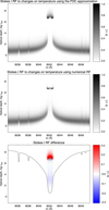 |
Fig. 1. Ca II 8542 Å Stokes I RF to changes in temperature. The top panel shows the RF computed using the FDC scheme implemented in DeSIRe, the middle panel shows the RF computed using the numerically evaluated NLTE RF, and the bottom panel displays the difference (normalised to the maximum of the numerical RF) between both computations. The intensity profile of the Ca II 8542 line is added in the bottom panel. |
3.3. Cycles, nodes, and equivalent response functions
From Sect. 2 we know that we need to specify the value of temperature T, electron pressure Pe, microturbulence ξ, line of sight (LOS) velocity VLoS, and magnetic field vector (B, γ, χ) at every reference optical depth τ500, to evaluate the emerging Stokes profiles and the RFs. In addition, to reproduce some observational features, we also included three additional uni-evaluated parameters that are not defined at every optical depth but are assumed constant throughout the atmosphere: the macroturbulence amplitude, Vmac, the filling factor, αf, and the stray light factor, αstr. We call this table of physical quantities our model atmosphere and denote it as xi = x(τi), where x stands for any physical quantity, T, B, and so on. We note that we do not need to specify the gas pressure Pg, nor gas density ρ since both are determined from T and Pe through the equation of state. In addition, geometrical height z can be derived by integration of Eq. (9).
The vertical domain of a typical atmospheric model ranges from log(τ500)∼[1, −8] with a step size of ∼0.1. Hence, a model atmosphere will contain around one hundred points in depth. In general, spectral lines will not be sensitive to fluctuations spanning a few steps in optical depth because the mean free path of a photon is larger than log(τ500)∼0.1. Consequently, a perturbation in any physical quantity with a very high spatial frequency will be undetectable. The inversion code works iteratively to determine the highest frequency fluctuation we should use, mimicking an expansion series. We call a single instance of these iterations an iterative cycle. Typically, a constant or linear perturbation through the whole atmosphere is specified in the first cycle; in the second one, a parabolic perturbation is added and further refinements are applied in successive cycles until appropriate convergence is reached.
We define as nodes those points in optical depth at which the perturbation of each cycle is evaluated, and let δxj = x(τj), with j = 1, ..., nnod, be those perturbations in physical quantities evaluated at these nodes j. The perturbations in the intermediate depth points will be obtained after the following interpolation:
 (51)
(51)
where aij are the interpolation coefficients. In general these are obtained through cubic spline interpolation.
We can introduce the δxi expression in Eq. (46):
 (52)
(52)
where  are the equivalent response functions (ERFs) at the nodes:
 (53)
(53)
These ERFs are the ones DeSIRe uses during an inversion process (i.e. the code only computes the RF and solves the RTE on the optical depth points where we have defined a node). For the remaining optical depths DeSIRe interpolates the solution (i.e. the atmospheric parameters) between these nodes.
3.4. Inversion based on response functions
DeSIRe combines the capabilities of SIR and RH to solve the inversion of the Stokes parameters in NLTE in a fast and flexible way. The flow chart of the inversion module consists of the following six steps.
First, the code reads the observed Stokes profiles Iobs; the initial guess model atmosphere aij(τ), where i is the iteration index (0 in the case of the ‘initial guess’ model); j runs for every physical quantity for one or two model atmospheres (temperature, electronic pressure, magnetic field vector, LOS velocity, micro- and macro-turbulence velocities, filling factor and stray light contamination factor); the atomic models; and all the information required to synthesise the Stokes profile vector.
Second, using RH’s subroutines, DeSIRe synthesises Iisyn = IiNLTE in NLTE computing the departure coefficients βup and βlow from the atmospheric model ai for every transition line. The computation is done including multiple atoms and molecules, and considering complete or partial redistribution (CRD or PRD) for the transitions of interest. Using SIR subroutines, it synthesises IiSIR in LTE and the approximated RFs (i.e. the LTE ones corrected by the FDCs and the ratio of the emission profile over the absorption profile, ψ/ϕ) for every spectral line specified by the user.
Third, with these RFs, the SIR module makes an inversion iteration minimising the χ2 (i.e. the total squared difference between Iobs and Iisyn) and delivers a new atmospheric model, ai + k, and the respective profile, Ii + kSIR (with k = 1 in this first step).
Fourth, if the maximum temperature difference between ai + k and ai is lower than a threshold specified by the user (we recommend a threshold of 10% of the maximum value of the temperature), the code will start an LTE cycle, updating the RFs for every new model while keeping the departure coefficients constant. During this cycle the code minimises the total squared difference between Iobs and  . This iteration will run, increasing k until the temperature perturbation exceeds the threshold, until k reaches a given maximum, or until the χ2 reaches the desired target.
Fifth, when the temperature perturbation exceeds the given threshold for temperature changes, it goes back to step 2, increasing i and re-evaluating the departure coefficients and Iisyn = IiNLTE using RH.
Finally, once the code ends executing the previous points, it evaluates a final Isyn = INLTE running RH from the final atmospheric model aj(τ).
Following these steps, the code can solve the NLTE inversion problem minimising the total number of calls to the NLTE transfer problem in order to reduce computational demands. The crucial element in the DeSIRe flow chart is the temperature threshold. Should this threshold be stringent (i.e. requiring an absolute change in temperature of e.g., less than 1% between iterations), DeSIRe will run RH internally a large number of times to re-evaluate the FDCs. If it is set to a less stringent condition (i.e. requiring that temperature changes by an absolute difference of less than 10–15%), the number of calls to RH is much reduced. Also, as an extra note, we want to clarify the meaning of IiSIR, used in the previous description. If DeSIRe runs in LTE mode, for example if we are inverting only photospheric lines, then that intensity is the one generated by SIR, with no DC correction. If the code runs in NLTE, that intensity can correspond to two different values. If we have started step 2, then that intensity corresponds to the one generated by SIR, evaluated from the opacity and source function corrected by the departure coefficients from RH. If we are in step 4, that intensity corresponds to the one generated by SIR from the atmosphere ai + k corrected with the DC from the latest call to RH.
Integrating RH and SIR within the same code has particular difficulties, the two most important of which are as follows. First, SIR and RH employ different opacity packages. However, DeSIRe always uses the NLTE profiles calculated by RH and its opacity package, whereas the only quantities calculated using the opacity package of SIR are the LTE RFs. Second, RH and SIR originally used different RTE solvers, while in DeSIRe the RH and SIR modules have been updated to work with the very same RTE solver (i.e. the DELO-Bezier formal solution presented in de la Cruz Rodríguez et al. 2013).
Finally, large datasets with many pixels can be inverted extremely efficiently on massively parallel compute clusters by employing the Python wrapper presented in Gafeira et al. (2021) with DeSIRe.
4. Numerical experiments
During the development of DeSIRe, it was extensively tested with different atmospheric models and conditions to evaluate its robustness and accuracy. For clarity, we focus only on the tests performed with 3D realistic numerical simulations in this work since these allow us to directly compare the inversion results with the original atmosphere. We used snapshot 385 of the Enhanced Network simulation described in Carlsson et al. (2016) and developed with the Bifrost code (Gudiksen et al. 2011). The snapshot covers a surface of 24 × 24 Mm2 with a pixel size of 48 km, and a vertical domain ranging from 2.4 Mm below to 14.4 Mm above the continuum average optical depth unity at λ = 500 nm. The simulated scenario, albeit simpler than recent numerical simulations such as those presented in Hansteen et al. (2017, 2019) and Cheung et al. (2019), contains a configuration with strong network patches and quiet areas (see Fig. 2). The mentioned structures allow the capabilities of the spectral lines inversions to be ascertained from quiet-Sun spectropolarimetry. Moreover, the simulation is publicly available2, so the present work can be independently verified and allows our inversion results to be compared with those of different inversion codes.
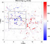 |
Fig. 2. Snapshot 385 from the Bifrost enhanced network simulation. We show the longitudinal component of the magnetic field strength at log τ500 = 0. We used two regions in this work, one within the squared box and the one highlighted with the horizontal line. |
We assumed disk centre observations (i.e. μ = 1, where μ = cos(θ) and θ the heliocentric angle). We used the abundance values of the different atomic species given in Asplund et al. (2009). We did not study the influence of noise or limited spatial and spectral resolution, and we did not include any microturbulence enhancement either. We are primarily interested in examining the code’s capabilities for inverting multiple lines in LTE and NLTE simultaneously.
4.1. Simulating DKIST level-2 ViSP observations
We study the accuracy of DeSIRe when inverting a large field of view (FOV) of the Bifrost simulation first (see the square in Fig. 2). The synthesis is done with DeSIRe after transforming the simulation to an optical depth grid. We focus in this section on the Fe I 630 nm line pair plus the two Ca II spectral windows presented below. These spectral regions are selected based on the plans for DKIST’s Visible Spectro-Polarimeter (ViSP, de Wijn et al. 2012, 2021) level-2 standard inversion products3. In addition, these spectral lines have been selected for spectropolarimetry with ViSP during the DKIST Cycle 1 Proposal Call. They will also be observed (in at least the red part of the spectrum) by the upcoming Sunrise Chromospheric Infrared Polarimeter (SCIP; Katsukawa et al. 2020) instrument that will operate on board the Sunrise (Solanki et al. 2010; Barthol et al. 2011) balloon’s third flight, programmed for 2022. Thus, we believe it is an excellent opportunity to test the code in this section focusing on their target spectrum. The atomic information of the strongest spectral lines in the selected spectral windows is shown in Table 1. The information was obtained from either the National Institute of Standards and Technology (NIST; Kramida et al. 2018) or the R. Kurucz (Kurucz & Bell 1995) databases. The broadening of the spectral lines by collisions with neutral hydrogen atoms is computed using the Anstee, Barklem, and O’Mara (ABO) theory (e.g., Anstee & O’Mara 1995; Barklem & O’Mara 1997), specifically the abo-cross calculator code (Barklem et al. 2015), which interpolates in pre-computed tables of line broadening parameters. A description of how to use the code can be found in Barklem et al. (1998).
4.2. Inversion configuration
We inverted the synthetic profiles computed with DeSIRe, starting from five possible initial guess atmospheres derived by applying linear perturbations to the FAL-C (Fontenla et al. 1993) atmosphere and using the set of nodes presented in Table 2. We pick the best fit from the converged solutions with five different initialisations.
Spectral lines included in the inversion test, representative of the DKIST/ViSP level 2 configuration proposal.
We performed two different tests using the previous configuration. First, we synthesise what we called ViSP level 2-like data where the spectral lines presented in Table 1 are used, solving the Ca II populations in NLTE. This inversion is done over the squared FOV highlighted in Fig. 2. In the second case, we performed the inversion of the pixels highlighted by the horizontal line enclosed by the square. In that case, we invert multiple atoms in NLTE to test the code capabilities and stability under these conditions.
4.3. DKIST level-2 ViSP configuration inversion test
The results of the inversion of the square subfield in Fig. 2 are shown in Fig. 3, where quantities in odd rows correspond to the original atmosphere at log τ500 = [0, −2, −5]4 while even rows display the inferred atmospheric quantities at the same optical depths. We can see that, in general, the resemblance between the original and inferred temperature, LOS velocity, and LOS magnetic field is very good. In particular, the values are almost identical in lower layers. In the case of upper layers, we see more differences. The code cannot accurately retrieve the temperature in the cool areas of the original atmosphere (first column, τ500 = −5), although it is more accurate in reproducing the velocity and magnetic field. Thus, taking into account that we are starting from a FALC atmosphere with the LOS velocity and the magnetic field vector constant with height, we believe the code is behaving well and is retrieving a solution that is close to the original one (despite the finite number of nodes used in the process).
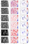 |
Fig. 3. Comparison between the input atmosphere (odd rows) and the one inferred with DeSIRe (even rows). From left to right, we show the temperature, the LOS velocity, and the magnetic field. From top to bottom, we display the atmospheric parameters at three reference layers at log τ500 = [0, −2, −5]. The FOV corresponds to the spatial domain within the squared region in Fig. 2. |
We note that the averaged inversion time per pixel is 5 minutes on a standard 2.1 GHz type CPU, i.e. Xeon Gold 6152. So, the code is capable of inverting the whole 230 × 230 pixel subfield in a little over 3 hours on a 1000 CPU cluster, showing that the speed of the DeSIRe code is suitable for inverting large DKIST FOVs in a reasonable time.
To illustrate the good correspondence between original atmospheric quantities and the results of the inversion, we show their correlation as a function of height in Fig. 4. We note that we are matching on average the input atmosphere in lower layers, but that the correlation drops in higher layers, above log τ500 = −3. This reduction of the correlation can be due to several factors; the assumptions in the code itself, the inversion configuration, or the limited sensitivity of the employed spectral lines to properties of the different layers. In particular, the LTE lines are sensitive below log τ500 ≈ −2.5, while the two Ca II infrared lines are most sensitive at layers deeper than log τ500 ≈ −5.0 (Quintero Noda et al. 2017) so there is a region in between where the spectral lines we employ in this setup are less sensitive. Accordingly, we can see a slight decrease in the correlation for all the atmospheric parameters between log τ500 ≈ [ − 3, −5]. We believe the drop is due to the gap in the sensitivity between the iron lines and the calcium lines in the infrared. We complement the previous analysis by plotting the average values for each optical depth of the difference between the input and the inferred atmosphere in the bottom row of the same figure. We add an error bar that corresponds to the standard deviation of the same difference over the entire FOV for each optical depth. The results are in agreement with what we explained above, with the differences close to zero in general between log τ500 ≈ [0, −5]. Only the temperature shows larger discrepancies above log τ500 ≈ −4.5. We believe those more significant differences correspond to the cool areas on the input atmosphere that our inversion run could not match (see Fig. 3).
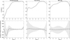 |
Fig. 4. Accuracy of the inversion code for inferring complex atmospheres. The top row displays the correlation between the input and the inferred atmospheric parameters presented in Fig. 3. The bottom row shows the average value of the difference between the input and the inferred atmosphere over the entire inverted FOV. Error bars designate the standard deviation of the difference. From left to right, columns correspond to the temperature, LOS velocity, and LOS magnetic field. Each panel displays the variation in the correlation and differences with optical depth. |
To show the code’s capability to achieve close fits to all employed LTE and NLTE spectral lines, we examined one pixel in detail. We chose a pixel where the magnetic field stratification is complex, that is, the magnetic field is weak at lower layers and gets stronger at higher heights. This pixel seems to be representative of the canopy effect. It is located at [6.2,12.6] Mm in Fig. 2, and it also has a temperature and LOS velocity stratification that vary on a small spatial scale. Thus, we believe it is a good benchmark of the code behaviour and the configuration used in this test. In Fig. 5, we show the original values of temperature, LOS velocity and LOS magnetic field (in black) and their recovered stratification (in red) for the selected pixel. We note that the inferred temperature traces with high accuracy the original atmosphere in most of the layers. There are slight differences at around log τ500 ≈ −4.3, but in general, the resemblance is very close. The same can be said for the LOS velocity, where the inferred values match the original ones up to log τ500 ≈ −5.5 before it deviates, probably due to the lack of sensitivity at the top of the atmosphere. The same behaviour is found in the LOS magnetic field, where the code tracks the original atmosphere at all heights (although with less accuracy at log τ500 ≈ −4.7). Thus, we confirm that the code is working correctly and recovers the input atmosphere with high accuracy. Since we can directly compare inverted values with the original atmospheric quantities, we do not show any estimates of the uncertainty in these graphs. However, in the future, when processing actual observations, the uncertainty of the inversion results can, for instance, be computed from the maximum amplitude of the total RF (all spectral lines combined) at each optical depth.
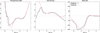 |
Fig. 5. Stratification of temperature, LOS velocity, and LOS magnetic field (from left to right) in one pixel. Black indicates the original physical parameters used during the synthesis, and red designates the inferred atmospheres using the configuration explained in Sect. 4. The pixel is located at [6.2, 12.6] Mm in Fig. 2. |
We display in Fig. 6 the comparison between the original forward calculated Stokes parameters (in black) of the selected pixel with the values from the inversion (in red) in all three spectral bands, centred on the Fe I, Ca II 8498 Å, and Ca II 8542 Å lines, respectively. The code fits the Stokes I and V profiles very accurately in all three bands (including the overlapping photospheric line in the calcium triplet bands, apart from perhaps the V profile of the 8542 Å line), explaining why the temperature and LOS velocity and magnetic field are reproduced very well in all layers. The amplitudes of the linear polarisation signals, Q and U are slightly less well produced, indicating that the inferred orientation of the magnetic field would be less accurately recovered. We further explore the accuracy of the fits of the chromospheric lines, in particular the Ca II 8542 Å in Fig. 7. There, we zoom in on the spectral range analysed in Fig. 6 to understand better the similarities between the original forward calculated Stokes profiles (black) and those inferred from the inversion (red). In general, we can see that, as mentioned above, the code is obtaining similar profiles to the original ones, even being complex ones with multiple lobes with different amplitude. Although it is true that the fit of the linear polarisation signals is worse than that of Stokes I and V.
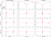 |
Fig. 6. Stokes (I, Q, U, V) parameters (from top to bottom) for the Fe I 6301.5 \AMP 6302.5 Å (left), Ca II 8498 Å (middle), and Ca II 8542 Å (right) spectral lines. Black designates the original Stokes profiles, and red corresponds to the inferred spectra using the configuration explained in Sect. 4. The pixel is located at [6.2,12.6] Mm in Fig. 2, and the associated atmosphere is presented in Fig. 5. |
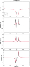 |
Fig. 7. Zoomed-in view of the Ca II 8542 Å Stokes profiles presented in Fig. 6. The format is the same. |
Therefore, the code can fit the diverse set of spectral lines very well at all wavelengths, indicating that this setup is very well suited to simultaneously recovering atmospheric properties in both the photosphere and chromosphere. It is thus very well suited to analyse data from the DKIST/ViSP instrument (with its three arms configured to observe all three spectral bands employed here) and the Sunrise/SCIP instrument observing the 8498 and 8542 Å bands (Katsukawa et al. 2020).
4.4. Multi-atom inversion test
The strategy for synthesis and inversion in this section is the same as before. However, we changed the spectral lines of interest. We only synthesised two photospheric lines in LTE: the Fe I ones at 6301.5 and 6302.5 Å and we combine them with multiple NLTE transitions to test the accuracy and speed of the code. We compute the Mg I b lines, the Na I and K I D1 \AMP D2 lines, and the Ca II 8498 and 8542 Å lines in NLTE. For the Mg spectral lines, we use the atom model presented in Quintero Noda et al. (2018). We employ the atom models included with RH’s source code distribution for the rest of the transitions.
We present the multi-atom inversion results in Fig. 8 using a vertical cut through the atmosphere (corresponding to the horizontal line in Fig. 2, with the depth scale in log τ500). We aim to examine the height stratification of the atmospheric parameters using multiple NLTE transitions with various heights of formation. Moreover, we want to evaluate the code’s capability for retrieving the smooth variation from pixel to pixel. We remark here that the code works under the 1.5D approximation, inverting pixel by pixel, and we have not included any regularisation between neighbouring pixels in the present version. In other words, DeSIRe does not have any information or pre-conditioning from adjacent pixels when inverting a given pixel. Thus, our motivation is to determine whether the code can recover the spatial smoothness of the original simulation.
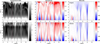 |
Fig. 8. Comparison between the input atmosphere (top) and the atmosphere inferred with DeSIRe (bottom) for the inversion test described in Sect. 4.4. From left to right, we show the temperature, the LOS velocity, and the magnetic field. The FOV corresponds to the horizontal line enclosed within the squared region in Fig. 2. Abscissae correspond to the X axis in Fig. 2, and ordinates show the evolution with the height of the atmospheric parameters. |
As in the previous test, we can see in Fig. 8 that the code is very reliable: the inferred atmospheric properties (bottom) closely match the original ones (top). We notice the impact of the discretisation of the inversion (see Table 2), but the height variation still resembles that of the original atmosphere. We also detect that upper layers above log τ500 ≈ −5.5 are recovered considerably less accurately, mainly in temperature. This results from the lack of sensitivity of the spectral lines in these layers, more than a failing of the code. Interestingly, we observe that complex magnetic field configurations are recovered in most cases, even where the field changes sign with height. Even if we do not add any regularisation in this version of the code, we also find a smooth transition between pixels. For instance, on the LOS velocity panels (middle), where the changes from upflows, null velocity, and downflows are preserved with high accuracy in the inferred atmospheres (taking into account that we are starting the inversion with a constant LOS velocity and magnetic field). Finally, we show in Fig. 9 an example of the accuracy of DeSIRe when inverting multiple NLTE spectral lines simultaneously. We only plot the intensity profile to reduce the number of graphs. The fits are very accurate, indicating that the code is stable even when combining such a variety of spectral lines and atomic models, forming in diverse ways.
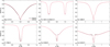 |
Fig. 9. Results from the multi-atom inversion test described in Sect. 4.4. Panels show the intensity, with black the input profile and red the inferred profile from DeSIRe. The pixel is located at X = 4 Mm in Fig. 2 (see dotted line). |
5. Summary and conclusions
This work presents a numerically highly efficient code for inverting polarimetric data of lines that form under general NLTE conditions. In particular, we describe how we combine the LTE inversion code SIR with the NLTE forward solver RH through the technique of FDCs (and fixed emission profiles in the case of PRD lines) into our new code, DeSIRe. The SIR code employs RFs that can be derived analytically under LTE conditions. In DeSIRe, the RFs of NLTE lines are evaluated by correcting the analytical RFs as formulated for LTE conditions with the NLTE departure coefficients from RH. In a series of iterative steps, an initial guess atmosphere is corrected by alternately solving the general NLTE equation of radiative transfer with RH, handing the evaluated spectrum, the departure coefficients, and the emission profiles of relevant lines to SIR, and evaluating the NLTE-corrected RFs. These are then used in SIR to correct the guess atmosphere to improve the spectral line fit. This process is iterated until convergence is reached (i.e. a sufficiently close match between observed and modelled spectra). DeSIRe can invert NLTE lines of different atomic species simultaneously, solving the combined equations of radiative transfer and statistical equilibrium consistently, including the effects of partial frequency redistribution. Our experience is that the implemented inversion process is stable and efficient. It is worth noting that while the FDC method assumes that the derivatives of the departure coefficients (and the emission profile in the case of PRD) with respect to the atmospheric parameters that need to be determined are negligible, this approximation is only used for the convergence process. The final solution, once converged, reflects the fully consistent simultaneous solution of the NLTE equations of both radiative transfer and statistical equilibrium.
We describe several numerical tests in Sect. 4 that we used to validate the performance of the new code. Starting from a snapshot of a Rad-MHD simulation of solar convection that includes chromospheric physics (Fig. 2), we calculated the emergent spectra in three wavelength bands centred around the Fe I 6300 Å doublet and the Ca II 8498 and 8542 Å IR triplet lines, respectively. Then, starting from a series of five initial atmospheres derived from the FALC standard quiet-Sun model, we inverted all lines in the three bands and compared the stratification of the derived physical parameters with the original values in each pixel. In a second test, we performed the same type of exercise in a vertical slice (see the horizontal marking line in Fig. 2) of the same snapshot, but using a different line set that includes spectral lines from multiple atomic species (Ca II, Mg I, Na I, and KI) in NLTE. We limited ourselves here to these numerical experiments for verification purposes of accuracy and reliability, deferring tests on actual data to a later paper.
In both test cases, we find that DeSIRe is able to accurately fit the line profiles in all lines and all four Stokes parameters (Figs. 6 and 9) and accordingly is able to recover the physical parameters from the spectra reliably. In both cases, we find that the most significant deviations between inverted and original temperatures occur at the top of the atmosphere, for logτ500 < −5 (see Figs. 4 and 8), but we ascribe that more to the physics of the formation of scattering lines in the chromosphere, the emergent intensity of which has inherently limited sensitivity to local thermodynamic conditions, than to a failure of the implemented inversion mechanism.
In our test, we find that a typical NLTE inversion takes 2-5 min on a modern 2.1 GHz CPU, making the inversion process significantly faster than for inversion techniques that employ numerical RFs, and making clear that we have achieved our goal of building an efficient and robust inversion engine. The efficiency of the new code, combined with the parallel Python wrap that enables the distribution of the inversion process in individual, independent pixels over the CPUs of massively parallel computers, provides us with the promise that we can manage the inversion of large high-resolution datasets in a timely manner.
The DeSIRe code is open and publicly available in the GitHub repository5.
It is important to bear in mind that none of the codes presented here infer the RFs fully analytically from the mathematical point of view since the solution of the RTE is always a numerical problem. Only in simplified atmospheres, as in a Milne-Eddington approximation, this would be strictly valid. Hence, we refer to numerical RFs when they are computed using finite difference methods.
We always refer to the optical depth at 500 nm when using log τ500.
Acknowledgments
C. Quintero Noda was supported by the EST Project Office, funded by the Canary Islands Government (file SD 17/01) under a direct grant awarded to the IAC on ground of public interest. This activity has also received funding from the European Union’s Horizon 2020 research and innovation programme under grant agreement No 739500. C. Quintero Noda also acknowledges the support of the ISAS/JAXA International Top Young Fellowship (ITYF) and the JSPS KAKENHI Grant Number 18K13596. This work was supported by ISAS/JAXA Small Mission-of-Opportunity program for novel solar observations and JSPS KAKENHI Grant Number JP18H05234. This work was supported by the Research Council of Norway through its Centres of Excellence scheme, project number 262622, and through grants of computing time from the Programme for Supercomputing. This work was supported by Fundação para a Cióncia e a Tecnologia (FCT) through the research grants UIDB/04434/2020 and UIDP/04434/2020. This work has also been supported by Spanish Ministry of Economy and Competitiveness through the project ESP-2016-77548-C5-1-R and RTI2018-096886-B-C53. D. Orozco Suárez also acknowledges financial support through the Ramón y Cajal fellowships. CITEUC is funded by National Funds through FCT-Foundation for Science and Technology (project: UID/Multi/00611/2013) and FEDER - European Regional Development Fund through COMPETE 2020 Operational Programme Competitiveness and Internationalization (project: POCI-01-0145-FEDER-006922). NSO is operated by the Association of Universities for Research in Astronomy (AURA), Inc. under cooperative agreement with the National Science Foundation (NSF).
References
- Anstee, S. D., & O’Mara, B. J. 1995, MNRAS, 276, 859 [Google Scholar]
- Asplund, M., Grevesse, N., Sauval, A. J., & Scott, P. 2009, ARA&A, 47, 481 [NASA ADS] [CrossRef] [Google Scholar]
- Barklem, P. S., & O’Mara, B. J. 1997, MNRAS, 290, 102 [Google Scholar]
- Barklem, P. S., Anstee, S. D., & O’Mara, B. J. 1998, PASA, 15, 336 [Google Scholar]
- Barklem, P. S., Anstee, S. D., & O’Mara, B. J. 2015, Astrophysics Source Code Library [record ascl:1507.007] [Google Scholar]
- Barthol, P., Gandorfer, A., Solanki, S. K., et al. 2011, Sol. Phys., 268, 1 [Google Scholar]
- Carlsson, M., Hansteen, V. H., Gudiksen, B. V., Leenaarts, J., & De Pontieu, B. 2016, A&A, 585, A4 [NASA ADS] [CrossRef] [EDP Sciences] [Google Scholar]
- Cheung, M. C. M., Rempel, M., Chintzoglou, G., et al. 2019, Nat. Astron., 3, 160 [NASA ADS] [CrossRef] [Google Scholar]
- Collados, M., Bettonvil, F., Cavaller, L., et al. 2013, Mem. Soc. Astron. It., 84, 379 [NASA ADS] [Google Scholar]
- de la Cruz Rodríguez, J., Socas-Navarro, H., Carlsson, M., & Leenaarts, J. 2012, A&A, 543, A34 [Google Scholar]
- de la Cruz Rodríguez, J., De Pontieu, B., Carlsson, M., & Rouppe van der Voort, L. H. M. 2013, ApJ, 764, L11 [CrossRef] [Google Scholar]
- de la Cruz Rodríguez, J., Leenaarts, J., & Asensio Ramos, A. 2016, ApJ, 830, L30 [Google Scholar]
- de la Cruz Rodríguez, J., & van Noort, M. 2017, Space Sci. Rev., 210, 109 [Google Scholar]
- de la Cruz Rodríguez, J., Leenaarts, J., Danilovic, S., & Uitenbroek, H. 2019, A&A, 623, A74 [Google Scholar]
- del Toro Iniesta, J. C. 2003, Introduction to Spectropolarimetry (Cambridge, UK: Cambridge University Press) [Google Scholar]
- del Toro Iniesta, J. C., & Ruiz Cobo, B. 2016, Liv. Rev. Sol. Phys., 13, 4 [Google Scholar]
- de Wijn, A. G., Casini, R., Nelson, P. G., & Huang, P. 2012, in Ground-based and Airborne Instrumentation for Astronomy IV, eds. I. S. McLean, S. K. Ramsay, & H. Takami, SPIE Conf. Ser., 8446, 84466X [NASA ADS] [Google Scholar]
- de Wijn, A. G., de la Cruz Rodríguez, J., Scharmer, G. B., Sliepen, G., & Sütterlin, P. 2021, AJ, 161, 89 [NASA ADS] [CrossRef] [Google Scholar]
- Fontenla, J. M., Avrett, E. H., & Loeser, R. 1993, ApJ, 406, 319 [Google Scholar]
- Gafeira, R., Orozco Suárez, D., Milic, I., et al. 2021, A&A, 651, A31 [NASA ADS] [CrossRef] [EDP Sciences] [Google Scholar]
- Gingerich, O., Noyes, R. W., Kalkofen, W., & Cuny, Y. 1971, Sol. Phys., 18, 347 [Google Scholar]
- Gudiksen, B. V., Carlsson, M., Hansteen, V. H., et al. 2011, A&A, 531, A154 [NASA ADS] [CrossRef] [EDP Sciences] [Google Scholar]
- Hansteen, V. H., Archontis, V., Pereira, T. M. D., et al. 2017, ApJ, 839, 22 [NASA ADS] [CrossRef] [Google Scholar]
- Hansteen, V., Ortiz, A., Archontis, V., et al. 2019, A&A, 626, A33 [NASA ADS] [CrossRef] [EDP Sciences] [Google Scholar]
- Katsukawa, Y., del Toro Iniesta, J. C., Solanki, S. K., et al. 2020, SPIE Conf. Ser., 11447, 114470Y [NASA ADS] [Google Scholar]
- Kramida, A., Ralchenko, Y., Reader, J., & NIST ASD Team 2018, NIST Atomic Spectra Database (version 5.6.1), http://physics.nist.gov/asd [Google Scholar]
- Kurucz, R. L., & Bell, B. 1995, Atomic Line List (Cambridge, MA: Smithsonian Astrophysical Observatory) [Google Scholar]
- Landi Degl’Innocenti, E. 1976, A&AS, 25, 379 [NASA ADS] [Google Scholar]
- Landi Degl’Innocenti, E., & Landi Degl’Innocenti, M. 1977, A&A, 56, 111 [NASA ADS] [Google Scholar]
- Landi Degl’Innocenti, E., & Landi Degl’Innocenti, M. 1981, Nuovo Cimento B Serie, 62B, 1 [Google Scholar]
- Landi Degl’Innocenti, E., & Landi Degl’Innocenti, M. 1985, Sol. Phys., 97, 239 [Google Scholar]
- Landi Degl’Innocenti, E., & Landolfi, M. eds. 2004, Polarization in Spectral Lines, 307, Astrophysics and Space Science Library (Dordrecht: Kluwer Academic Publishers) [Google Scholar]
- Mihalas, D. 1978, Stellar Atmospheres (San Francisco: W.H. Freeman) [Google Scholar]
- Milić, I., & van Noort, M. 2017, A&A, 601, A100 [NASA ADS] [CrossRef] [EDP Sciences] [Google Scholar]
- Milić, I., & van Noort, M. 2018, A&A, 617, A24 [Google Scholar]
- Quintero Noda, C., Shimizu, T., de la Cruz Rodríguez, J., et al. 2016, MNRAS, 459, 3363 [Google Scholar]
- Quintero Noda, C., Shimizu, T., Katsukawa, Y., et al. 2017, MNRAS, 464, 4534 [NASA ADS] [CrossRef] [Google Scholar]
- Quintero Noda, C., Villanueva, G. L., Katsukawa, Y., et al. 2018, A&A, 610, A79 [NASA ADS] [CrossRef] [EDP Sciences] [Google Scholar]
- Rimmele, T. R., Warner, M., Keil, S. L., et al. 2020, Sol. Phys., 295, 172 [Google Scholar]
- Ruiz Cobo, B., & del Toro Iniesta, J. C. 1992, ApJ, 398, 375 [Google Scholar]
- Ruiz Cobo, B., & del Toro Iniesta, J. C. 1994, A&A, 283, 129 [NASA ADS] [Google Scholar]
- Rybicki, G. B., & Hummer, D. G. 1992, A&A, 262, 209 [NASA ADS] [Google Scholar]
- Skumanich, A., & Lites, B. W. 1987, ApJ, 322, 473 [Google Scholar]
- Socas-Navarro, H., Ruiz Cobo, B., & Trujillo Bueno, J. 1998, ApJ, 507, 470 [NASA ADS] [CrossRef] [Google Scholar]
- Socas-Navarro, H., Trujillo Bueno, J., & Ruiz Cobo, B. 2000, ApJ, 530, 977 [NASA ADS] [CrossRef] [Google Scholar]
- Socas-Navarro, H., de la Cruz Rodríguez, J., Asensio Ramos, A., Trujillo Bueno, J., & Ruiz Cobo, B. 2015, A&A, 577, A7 [NASA ADS] [CrossRef] [EDP Sciences] [Google Scholar]
- Solanki, S. K., Barthol, P., Danilovic, S., et al. 2010, ApJ, 723, L127 [NASA ADS] [CrossRef] [Google Scholar]
- Uitenbroek, H. 2001, ApJ, 557, 389 [Google Scholar]
- Uitenbroek, H. 2003, ApJ, 592, 1225 [Google Scholar]
- Uitenbroek, H. 2006, in Solar MHD Theory and Observations: A High Spatial Resolution Perspective, eds. J. Leibacher, R. F. Stein, & H. Uitenbroek, ASP Conf. Ser., 354, 313 [NASA ADS] [Google Scholar]
All Tables
Spectral lines included in the inversion test, representative of the DKIST/ViSP level 2 configuration proposal.
All Figures
|
Fig. 1. Ca II 8542 Å Stokes I RF to changes in temperature. The top panel shows the RF computed using the FDC scheme implemented in DeSIRe, the middle panel shows the RF computed using the numerically evaluated NLTE RF, and the bottom panel displays the difference (normalised to the maximum of the numerical RF) between both computations. The intensity profile of the Ca II 8542 line is added in the bottom panel. |
| In the text | |
|
Fig. 2. Snapshot 385 from the Bifrost enhanced network simulation. We show the longitudinal component of the magnetic field strength at log τ500 = 0. We used two regions in this work, one within the squared box and the one highlighted with the horizontal line. |
| In the text | |
|
Fig. 3. Comparison between the input atmosphere (odd rows) and the one inferred with DeSIRe (even rows). From left to right, we show the temperature, the LOS velocity, and the magnetic field. From top to bottom, we display the atmospheric parameters at three reference layers at log τ500 = [0, −2, −5]. The FOV corresponds to the spatial domain within the squared region in Fig. 2. |
| In the text | |
|
Fig. 4. Accuracy of the inversion code for inferring complex atmospheres. The top row displays the correlation between the input and the inferred atmospheric parameters presented in Fig. 3. The bottom row shows the average value of the difference between the input and the inferred atmosphere over the entire inverted FOV. Error bars designate the standard deviation of the difference. From left to right, columns correspond to the temperature, LOS velocity, and LOS magnetic field. Each panel displays the variation in the correlation and differences with optical depth. |
| In the text | |
|
Fig. 5. Stratification of temperature, LOS velocity, and LOS magnetic field (from left to right) in one pixel. Black indicates the original physical parameters used during the synthesis, and red designates the inferred atmospheres using the configuration explained in Sect. 4. The pixel is located at [6.2, 12.6] Mm in Fig. 2. |
| In the text | |
|
Fig. 6. Stokes (I, Q, U, V) parameters (from top to bottom) for the Fe I 6301.5 \AMP 6302.5 Å (left), Ca II 8498 Å (middle), and Ca II 8542 Å (right) spectral lines. Black designates the original Stokes profiles, and red corresponds to the inferred spectra using the configuration explained in Sect. 4. The pixel is located at [6.2,12.6] Mm in Fig. 2, and the associated atmosphere is presented in Fig. 5. |
| In the text | |
|
Fig. 7. Zoomed-in view of the Ca II 8542 Å Stokes profiles presented in Fig. 6. The format is the same. |
| In the text | |
|
Fig. 8. Comparison between the input atmosphere (top) and the atmosphere inferred with DeSIRe (bottom) for the inversion test described in Sect. 4.4. From left to right, we show the temperature, the LOS velocity, and the magnetic field. The FOV corresponds to the horizontal line enclosed within the squared region in Fig. 2. Abscissae correspond to the X axis in Fig. 2, and ordinates show the evolution with the height of the atmospheric parameters. |
| In the text | |
|
Fig. 9. Results from the multi-atom inversion test described in Sect. 4.4. Panels show the intensity, with black the input profile and red the inferred profile from DeSIRe. The pixel is located at X = 4 Mm in Fig. 2 (see dotted line). |
| In the text | |
Current usage metrics show cumulative count of Article Views (full-text article views including HTML views, PDF and ePub downloads, according to the available data) and Abstracts Views on Vision4Press platform.
Data correspond to usage on the plateform after 2015. The current usage metrics is available 48-96 hours after online publication and is updated daily on week days.
Initial download of the metrics may take a while.