| Issue |
A&A
Volume 692, December 2024
|
|
|---|---|---|
| Article Number | A169 | |
| Number of page(s) | 7 | |
| Section | The Sun and the Heliosphere | |
| DOI | https://doi.org/10.1051/0004-6361/202452233 | |
| Published online | 12 December 2024 | |
Non-local thermodynamic equilibrium inversions of the Si I 10827 Å spectral line
1
Instituto de Astrofísica de Canarias, E-38205 La Laguna, Tenerife, Spain
2
Departamento de Astrofísica, Univ. de La Laguna, La Laguna, Tenerife E-38200, Spain
3
Main Astronomical Observatory, National Academy of Sciences, 03143 Kyiv, Ukraine
⋆ Corresponding author; This email address is being protected from spambots. You need JavaScript enabled to view it.
Received:
13
September
2024
Accepted:
16
November
2024
Abstract
Inferring the coupling of different atmospheric layers requires observing spectral lines sensitive to the atmospheric parameters, particularly the magnetic field vector, at various heights. The best way to tackle this goal is to perform multi-line observations simultaneously. For instance, the new version of the Gregor Infrared Spectrograph instrument offers the possibility to observe the spectral lines at 8542 and 10830 Å simultaneously for the first time. The first spectral window contains the Ca II 8542 Å spectral line, while the Si I 10827 Å transition and He I 10830 Å triplet infrared lines can be found in the second spectral window. As the sensitivity to the atmospheric parameters and the height of formation of those transitions is different, combining them can help understand the properties of the solar photosphere and chromosphere and how they are magnetically coupled. Traditionally, the analysis of the Si I 10827 Å transition assumes local thermodynamic equilibrium (LTE), which is not the best approximation to model this transition. Hence, in this work, we examine the potential of performing non-LTE (NLTE) inversions of the full Stokes vector of the Si I 10827 Å spectral line. The results indicate that we properly infer the atmospheric parameters through an extended range of atmospheric layers in comparison with the LTE case (only valid for the spectral line wings, i.e., the low photosphere), with no impact on the robustness of the solution and just a minor increase in computational time. Thus, the NLTE assumption will help to accurately constrain the photospheric physical parameters when performing combined inversions with, e.g., the Ca II 8542 Å spectral line.
Key words: radiative transfer / techniques: high angular resolution / techniques: polarimetric / Sun: chromosphere / Sun: magnetic fields
© The Authors 2024
 Open Access article, published by EDP Sciences, under the terms of the Creative Commons Attribution License (https://creativecommons.org/licenses/by/4.0), which permits unrestricted use, distribution, and reproduction in any medium, provided the original work is properly cited.
This article is published in open access under the Subscribe to Open model. This email address is being protected from spambots. You need JavaScript enabled to view it. to support open access publication.
1. Introduction
Understanding solar phenomena requires access to the physical parameters over a particular spatial domain and a specific range of atmospheric heights. The reason is that solar phenomena, particularly their magnetic field, can extend vertically (with respect to the solar surface) several hundred kilometres. Hence, to understand how the magnetic field is connected and structured along different atmospheric layers, we need to analyse spectral lines sensitive to the atmospheric parameters over such a range of heights. The best strategy is to simultaneously analyse spectral lines with different sensitivities to the atmospheric parameters and height of formation. In this regard, multi-line spectropolarimetric observations are the most common strategy to fulfil the mentioned requirement. The large-scale solar telescopes Daniel K. Inouye Solar Telescope (Rimmele et al. 2020) and the future European Solar Telescope (Quintero Noda et al. 2022a) have been designed to offer these multi-line configurations. In addition, instruments such as the Gregor Infrared Spectrograph (GRIS, Collados et al. 2012) installed at the Gregor telescope (Schmidt et al. 2012) have been recently upgraded to support multi-channel observations of complementary spectral lines (Quintero Noda et al. 2022b). In particular, GRIS was upgraded to observe simultaneously Ca II 8542 Å, with high sensitivity to the atmospheric parameters in the lower and middle chromosphere (see, for instance, Quintero Noda et al. 2016), and the He I 10830 Å infrared triplet whose formation properties make them ideal to examine targets such as filaments, spicules, and prominences.
Additionally, the spectral window at 10830 Å also contains the Si I 10827 Å transition. This strong photospheric line can complement the other two transitions when inferring the properties of the magnetic field at photospheric layers. However, although an accurate determination of the atomic populations of the silicon transition requires solving the radiative transfer equation under non-local thermodynamic equilibrium (NLTE, e.g., Bard & Carlsson 2008; Sukhorukov & Shchukina 2012; Shchukina et al. 2017; Shchukina & Trujillo Bueno 2019) the spectral line has usually been treated under the local thermodynamic equilibrium (LTE) formalism (with some exceptions such as in Orozco Suárez et al. 2017) when performing inversions (see, for instance, Kuckein et al. 2012a; Felipe et al. 2018; Díaz Baso et al. 2019). The main reason for this is that certain atoms, such as iron, calcium, or silicon, require a large number of atomic levels and transitions for their accurate modelling (particularly in the case of the minority species of the atom), which results in atomic models that are computationally expensive to work with. In order to reduce the computational burden, hybrid methods have been used in the past. For instance, Kuckein et al. (2012b) used NLTE departure coefficients computed with the atomic model presented in Bard & Carlsson (2008). In this case, the authors used a set of fixed departure coefficients to study the differences between a pure LTE inversion and one corrected by the mentioned departure coefficients. Their findings revealed no noticeable differences between LTE and NLTE for the magnetic field inclination and azimuth, while more significant variations were detected for the magnetic field strength. Moreover, the authors explained that even more prominent differences between LTE and NLTE were found for the inferred temperature.
In preparation for the observations that GRIS has already started (Quintero Noda et al. 2024) and those soon to be provided by the Diffraction Limited Near-Infrared Spectropolarimeter (DL-NIRSP; Jaeggli et al. 2022) we aim to study the differences between LTE versus NLTE inversions of the Si I 10827 Å transition with the simplified model atom presented in Shchukina et al. (2017). The goal is to analyse whether there is an improvement in the inferred atmosphere, particularly the thermal atmospheric parameters when using such a simplified atom, quantify the increase in computational time, and evaluate the robustness of the inversion process to use it as a baseline for the analysis of future observations from GRIS and similar instruments.
2. Data and methodology
The main goal of this work is to examine the difference between performing inversions of synthetic spectra of the Si I 10827 Å transition under LTE and NLTE conditions. We used the Stokes Inversion code based on Response functions (SIR, Ruiz Cobo & del Toro Iniesta 1992) for the LTE inversions and the Departure coefficient aided Stokes Inversion based on Response functions (DeSIRe; Ruiz Cobo et al. 2022) code for the NLTE inversions. The DeSIRe code can work both under the LTE and the NLTE approximation, but, as the reference inversions that have been done in the past for the Si I 10827 Å transition were done mainly with the SIR code, we believe it is appropriate to compare the inversion results from SIR with those from DeSIRe assuming NLTE.
To benchmark these inversions, we used two types of model atmospheres. We employed the semi-empirical atmosphere Harvard-Smithsonian Reference Atmosphere (HSRA; Gingerich et al. 1971) for comparing the main differences between the intensity profiles in LTE, NLTE, and the solar atlas. We also used the HSRA atmosphere for estimating the response functions (RF; see, e.g., Landi Degl’Innocenti & Landi Degl’Innocenti 1977) to perturbations of the atmospheric parameters in LTE and NLTE. We also employed a 3D realistic magneto-hydrodynamic (MHD) numerical simulation, specifically snapshot 385 of the enhanced network simulation1 described in Carlsson et al. (2016) and carried out with the Bifrost code (Gudiksen et al. 2011). The snapshot covers a field-of-view (FOV) of 24 × 24 Mm2 with a pixel size of 48 km, while the vertical domain extends from 2.4 Mm below to 14.4 Mm above the average height at which optical depth is unity at λ = 5000 Å.
We assumed disk centre observations, that is, μ = cos(θ) = 1, where θ is the heliocentric angle and considered the abundance values given in Asplund et al. (2009). We used a spectral sampling of 20 mÅ and degraded the synthetic Stokes profiles by adding noise with an amplitude of 5 × 10⁻⁴ of Ic. We preserved the original spatial resolution of 48 km per pixel, close to the value at the diffraction limit that Gregor could achieve at 10827 Å.
Regarding the atomic model for solving the atomic populations of the silicon transition, we used the simplest model presented in Shchukina et al. (2017). This simplest working model has 6 bound-bound radiative transitions between fine structure levels of the 4s 3Po (lower) and 4p 3P (upper) terms of Si I. One of these transitions, namely 4s 3P2o–4p 3P2, produces the transition of interest Si I 10827 Å. The model also includes the levels that play an important role in the ionization balance. They are low-excitation meta-stable levels of Si I lying below the 4s 3Po term, including their corresponding parent levels in the next ionization stage of Si II. In total, the simplest model has 16 levels, with twelve atomic energy levels of Si I, three levels from the 3p 2Po and 3p 4P terms of Si II, the ground level 3s 1S1 of Si III, that produce fifteen bound-free radiative transitions. We adapted the atom to be used with the RH code (Uitenbroek 2001, 2003) and made it publicly available2 so it can be used by any modern inversion code such as those presented in de la Cruz Rodríguez et al. (2019), del Pino Alemán et al. (2016), and Li et al. (2022).
3. Synthetic profiles
We examined the differences between solving the populations for the Si I 10827 Å transition in LTE versus NLTE. In particular, we made use of the HSRA atmosphere for the synthesis, and we compared the results with the atlas observed by Delbouille et al. (1973) and downloaded from the BAse de données Solaire Sol (BASS2000) archive3. Figure 1 shows the comparison between the three intensity profiles. The LTE profile generated with SIR (blue) matches the continuum and the wings of the line with high accuracy while it is far from the atlas at line core wavelengths. This was expected, as the spectral line is sensitive to NLTE effects (e.g., Sukhorukov & Shchukina 2012; Shchukina et al. 2017; Shchukina & Trujillo Bueno 2019). The NLTE intensity profile (red) generated with DeSIRe is very close to the atlas for all wavelengths, which is indicative of the suitability of the simplified atom for modelling the silicon transition.
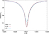 |
Fig. 1. Intensity profiles for the Si I 10827 Å transition from the solar atlas (black), LTE synthesis (blue), and an NLTE synthesis (red). Both syntheses were computed using the HSRA model atmosphere. |
We also analysed the differences between the LTE and NLTE RFs due to changes in different atmospheric parameters. Using the HSRA atmosphere, we computed the RFs analytically with SIR and numerically with DeSIRe following the method explained in Quintero Noda et al. (2016). The results are presented in Figure 2, where we show the maximum value of the RFs for all the wavelengths and the four Stokes parameters for the two approximations. Each RF is normalised to the maximum of the NLTE solution.
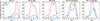 |
Fig. 2. Response functions to changes in the atmospheric parameters. From left to right, RFs to changes in temperature, line-of-sight velocity, and the three components of the magnetic field vector in polar coordinates. Each curve corresponds to the maximum value for the four Stokes parameters and all the computed wavelengths at each optical depth for the Si I 10827 Å spectral line. Blue and red designate the results from the LTE and NLTE solutions, respectively. RFs are normalised to the maximum value of the corresponding NLTE solution. |
The RFs to changes in temperature in NLTE and LTE are almost identical in the lower layers of the model. However, they deviate at higher layers, with the NLTE RF dropping its maximum value just before log τ = −3. This result indicates that the sensitivity of the Si I 10827 Å spectral line to temperature changes is only significant at the lower and middle photosphere. These results seem similar to those found for other spectral lines such us Na ID1 and D2 (e.g., Uitenbroek 2006), K ID1 and D2 (e.g., Quintero Noda et al. 2017; Alsina Ballester 2022), and the Mg I b transitions (e.g., Quintero Noda et al. 2018). Interestingly, the opposite behaviour is found for the rest of the RFs, with the NLTE RFs having non-negligible contributions at higher layers than those in LTE. These results indicate that we can expect that inverting the Si I 10827 Å spectral line in NLTE will provide better accuracy for the inferred parameters at higher layers.
In order to expand the previous studies that used 1D semi-empirical atmospheres, we used the enhanced network 3D simulation to study the impact of NLTE effects on the synthetic Stokes parameters. We first started synthesising the Stokes vector for the complete FOV of the simulation run. We show in Figure 3 the spatial distribution of the line core intensity signals, maximum linear polarisation signals (computed as  ) and maximum circular polarisation signals in absolute value. The spatial distribution of intensity signals (left column) shows a higher contrast for the NLTE computation (bottom row). This agrees with the results presented in Figure 1, where the line core intensity in NLTE is deeper than the LTE line core. The spatial distribution of polarisation signals (middle and rightmost column) shows larger amplitudes in the magnetised regions for the entire FOV. In addition, there is no apparent deviation between the two computations besides the mentioned ones, that is, the solar features seem to have the same shape and spatial distribution in both cases.
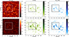 |
Fig. 3. Spatial distribution of spectral features. From left to right, we show the spatial distribution of line core intensity, maximum linear polarisation, and maximum circular polarisation signals for the Si I 10827 Å spectral line. The top row corresponds to the results from the LTE computation, while the bottom panels display the results of the NLTE case. The region enclosed by the white/black square corresponds to the FOV used for the inversion analysis in Section 4. |
4. Spectropolarimetric inversions
The main goal of this work is to ascertain whether we can improve the results obtained from LTE inversions of the Si I 10827 Å spectral line when using a simplified silicon atom to perform NLTE inversions. Additionally, two key elements are also essential. Firstly, we aim for an inversion process that is fast enough to be comparable to the LTE inversions. The NLTE inversion is always more time-consuming, but we aim for a small time difference. Secondly, we want the inversion process to be as robust as possible. It is well-known that NLTE inversions are more unstable than LTE inversions, so we want to check the fraction of pixels in which the inversion code did not reach an accurate convergence.
To tackle those questions, we performed inversions of all the pixels enclosed in the squared area highlighted in Figure 3. We selected this area because it is large enough to cover all the physical scenarios presented in the simulation, such as weakly magnetised areas and strongly magnetised ones. We used the synthetic profiles generated by DeSIRe and degraded with a noise contribution of 5 × 10⁻⁴ of Ic. These are the target profiles we fitted. As we were able to obtain good fits in both LTE and NLTE inversions, our accuracy estimation is directly how close the inferred atmospheres are to those used during the synthesis.
Table 1 shows the inversion configuration for the nodes. Each new column towards the rightmost side of the table adds (or maintains) more nodes for the inversion and corresponds to an additional inversion cycle. In addition, more information about the inversion strategy can be found in, for instance, Ferrente et al. (2024). As a reminder, the inversion code uses as free parameters the perturbations of the physical quantities on a specific grid of optical depth points (nodes), taking into account that the inferred atmosphere is the result of a high-order interpolation between those nodes (except in the case of 1 or 2 nodes, for which the interpolation is constant or linear, respectively). These free parameters are tuned to minimise the χ2 metric.
Number of nodes used for the inversion of each atmospheric parameter.
Regarding the physical quantities, we inferred the temperature, the line-of-sight (LOS) velocity, microturbulence, and the magnetic field vector. The inversion was done in multiple cycles, increasing the number of nodes for each atmospheric parameter as presented in Table 1, except for the microturbulence, which is always set to a constant. As a note, although no microturbulent velocity was used during the synthesis because it comes from a 3D MHD simulation that did not have any, we still added it as a free parameter in the inversions to account for the complicated vertical stratification in the LOS velocity and improve the accuracy of the inversion results (see the explanation in Sect. 3 of Milić et al. 2019, for more information).
The inversion was done in parallel using the Python-based wrapper described in Gafeira et al. (2021). This code allows the seamless utilisation of all available CPU cores to accelerate the inversion of many pixels. In addition, the wrapper can provide a set of atmospheres to initialise the inversion process, which allows initialising the inversion several times from different initial models and then picking the solution that achieves the best fit. This strategy helps in finding accurate solutions given the complexity of the χ2 hypersurface. Regarding the specific atmospheres used in the inversion as initialisation, they are created from the atmospheric models presented in Fontenla et al. (1993) and the HSRA atmosphere, adding small amplitude variations in the LOS velocity, microturbulence, and magnetic field (which are null in the original models). We created a library of 12 initial atmospheres with constant values with height for those physical parameters to initialise the inversion of each pixel.
As a first step, we examine the spatial distribution of the atmospheric parameters at selected atmospheric layers. The goal is to compare the main differences between the input atmosphere and those inferred, assuming LTE and NLTE, respectively. Figure 4 shows the results for the temperature. The spatial distribution of the inferred atmospheres is very close to the input simulation at log τ = 0 for both approximations. However, there are differences between the LTE and NLTE inversions in the middle and upper layers. At log τ = −1, the LTE inversion lacks contrast, while the NLTE inversion better resembles the input atmosphere. However, higher up, the LTE inversion is entirely different, indicating that the inferred atmospheres assuming LTE would only be accurate in the lower photosphere. In the case of NLTE inversions, there is a certain resemblance up to log τ = −3. However, at this height, the NLTE inversions cannot accurately reproduce the coolest regions, which translates into a lack of contrast with respect to the input atmosphere.
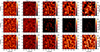 |
Fig. 4. Spatial variation of the temperature at different optical depths (columns from left to right). Rows display, from top to bottom, the original atmosphere, the one inferred assuming LTE and that from NLTE inversions, respectively. The spatial domain corresponds to that highlighted by the square in Figure 3. |
Regarding the LOS velocity, we detect a similar behaviour (see Figure 5). Results at around log τ = 0 are similar between LTE and NLTE, although the former shows systematically larger velocities. In this case, results at log τ = −1 are also good for both inversion schemes. Substantial deviations appear at log τ = −2, with the NLTE inversion closely resembling the input atmosphere up to log τ = −4 while the LTE solutions are less accurate. A similar behaviour is found for the magnetic field strength (Figure 6) and inclination (Figure 7). These results mean that the LTE inversion produces atmospheres that resemble the input simulation only at the lower atmosphere, below log τ = −2. In contrast, the NLTE inversion has better accuracy up to log τ ∼ −4.
In Figure 8, we show the average difference between the input atmosphere and that inferred, assuming LTE (blue) or NLTE (red). Except in some layers at the lower photosphere, the average difference for the LTE inversion is always worse than that from the NLTE inversions. Additionally, for the NLTE inversions, as predicted by the response function analysis shown in previous sections, the differences for temperature become large above log τ = −2. However, the differences remain small up to log τ ∼ −3 for the rest of the atmospheric parameters.
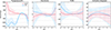 |
Fig. 8. Average differences between the input and the inferred atmosphere at different optical depths. From left to right, we show the differences in temperature, LOS velocity, magnetic field strength, and inclination. Colours correspond to the LTE case (blue) and NLTE assumption (red). Error bars display the standard deviation of the difference over the selected FOV at each optical depth. |
Finally, in terms of computational time, the average inversion time (just for a single atmospheric model) is 3.26 ± 0.56 s in LTE and 33.99 ± 6.03 s in NLTE. There is roughly an order of magnitude difference in computing time between the two approximations. In any case, with enough CPU cores, the inversion can be carried out in a relatively short time, allowing us to invert the selected FOV in a few hours. Moreover, it is also worth exploring solutions based on machine learning to accelerate the NLTE inversions (e.g., Vicente Arévalo et al. 2022; Chappell & Pereira 2022).
5. Summary
This work aimed to evaluate how much can be gained by performing NLTE inversions of the Si I 10827 Å spectral line using the simplest atom possible. The RFs indicate that the sensitivity of the NLTE solution extends to the upper photospheric layers as we correctly model the line core wavelengths of the transition in contrast with the LTE case. Interestingly, we also see that the NLTE inferred atmosphere remains accurate up to log τ ∼ −3 and slightly higher. In contrast, the LTE atmospheres are correct only at the lower photosphere, below log τ = −2, as this approximation is only valid for the wings of the spectral line. Also noteworthy is that the computational time increases from an average of 3 s in the LTE case to around 30 s for the NLTE inversions, a factor 10 that, although sizeable, is still smaller than the time needed to invert other NLTE spectral lines such as the Ca II infrared transitions. Consequently, its impact when inverting simultaneously several photospheric and chromospheric lines is much reduced. Finally, it is also critical that we see no effect on the robustness of the inversion, that is, no convergence issues were found in the NLTE inversion. Therefore, we conclude that the simplified silicon atom presented in Shchukina et al. (2017) is excellent for tackling the inversions of the Si I 10827 Å spectral line.
Finally, we plan to use this atom in the upcoming simultaneous observations of the spectral windows at 8542 and 10830 Å at the upgraded GRIS. This instrument will be offered publicly from the second semester of 2024. We believe the Si I 10827 Å spectral line is an excellent photospheric complement to the already capable Ca II 8542 Å transition, promising to increase the height resolution of the inferred atmospheric parameters and the sensitivity to quiet Sun magnetic fields in the lower atmosphere.
Acknowledgments
C. Quintero Noda, A. Asensio Ramos, T. del Pino Alemán, M. J. Martínez González, and J. C. Trelles Arjona acknowledge support from the Agencia Estatal de Investigación del Ministerio de Ciencia, Innovación y Universidades (MCIU/AEI) under grant “Polarimetric Inference of Magnetic Fields” and the European Regional Development Fund (ERDF) with reference PID2022-136563NB-I00/10.13039/501100011033. The publication is part of the Project ICTS2022-007828, funded by MICIN and the European Union NextGenerationEU/RTRP.
References
- Alsina Ballester, E. 2022, A&A, 666, A178 [NASA ADS] [CrossRef] [EDP Sciences] [Google Scholar]
- Asplund, M., Grevesse, N., Sauval, A. J., & Scott, P. 2009, ARA&A, 47, 481 [NASA ADS] [CrossRef] [Google Scholar]
- Bard, S., & Carlsson, M. 2008, ApJ, 682, 1376 [NASA ADS] [CrossRef] [Google Scholar]
- Carlsson, M., Hansteen, V. H., Gudiksen, B. V., Leenaarts, J., & De Pontieu, B. 2016, A&A, 585, A4 [NASA ADS] [CrossRef] [EDP Sciences] [Google Scholar]
- Chappell, B. A., & Pereira, T. M. D. 2022, A&A, 658, A182 [NASA ADS] [CrossRef] [EDP Sciences] [Google Scholar]
- Collados, M., López, R., Páez, E., et al. 2012, Astron. Nachr., 333, 872 [Google Scholar]
- de la Cruz Rodríguez, J., Leenaarts, J., Danilovic, S., & Uitenbroek, H. 2019, A&A, 623, A74 [Google Scholar]
- del Pino Alemán, T., Casini, R., & Manso Sainz, R. 2016, ApJ, 830, L24 [Google Scholar]
- Delbouille, L., Roland, G., & Neven, L. 1973, Atlas photometrique du spectre solaire de [lambda] 3000 a [lambda] 10000 (Liege: Universite de Liege) [Google Scholar]
- Díaz Baso, C. J., Martínez González, M. J., & Asensio Ramos, A. 2019, A&A, 625, A128 [NASA ADS] [CrossRef] [EDP Sciences] [Google Scholar]
- Felipe, T., Kuckein, C., & Thaler, I. 2018, A&A, 617, A39 [NASA ADS] [CrossRef] [EDP Sciences] [Google Scholar]
- Ferrente, F., Quintero Noda, C., Zuccarello, F., & Guglielmino, S. L. 2024, A&A, 686, A244 [NASA ADS] [CrossRef] [EDP Sciences] [Google Scholar]
- Fontenla, J. M., Avrett, E. H., & Loeser, R. 1993, ApJ, 406, 319 [Google Scholar]
- Gafeira, R., Orozco Suárez, D., Milić, I., et al. 2021, A&A, 651, A31 [NASA ADS] [CrossRef] [EDP Sciences] [Google Scholar]
- Gingerich, O., Noyes, R. W., Kalkofen, W., & Cuny, Y. 1971, Sol. Phys., 18, 347 [Google Scholar]
- Gudiksen, B. V., Carlsson, M., Hansteen, V. H., et al. 2011, A&A, 531, A154 [NASA ADS] [CrossRef] [EDP Sciences] [Google Scholar]
- Jaeggli, S. A., Lin, H., Onaka, P., et al. 2022, Sol. Phys., 297, 137 [NASA ADS] [CrossRef] [Google Scholar]
- Kuckein, C., Martínez Pillet, V., & Centeno, R. 2012a, A&A, 542, A112 [NASA ADS] [CrossRef] [EDP Sciences] [Google Scholar]
- Kuckein, C., Martínez Pillet, V., & Centeno, R. 2012b, A&A, 539, A131 [NASA ADS] [CrossRef] [EDP Sciences] [Google Scholar]
- Landi Degl’Innocenti, E., & Landi Degl’Innocenti, M. 1977, A&A, 56, 111 [NASA ADS] [Google Scholar]
- Li, H., del Pino Alemán, T., Trujillo Bueno, J., & Casini, R. 2022, ApJ, 933, 145 [NASA ADS] [CrossRef] [Google Scholar]
- Milić, I., Smitha, H. N., & Lagg, A. 2019, A&A, 630, A133 [Google Scholar]
- Orozco Suárez, D., Quintero Noda, C., Ruiz Cobo, B., Collados Vera, M., & Felipe, T. 2017, A&A, 607, A102 [NASA ADS] [CrossRef] [EDP Sciences] [Google Scholar]
- Quintero Noda, C., Shimizu, T., de la Cruz Rodríguez, J., et al. 2016, MNRAS, 459, 3363 [Google Scholar]
- Quintero Noda, C., Uitenbroek, H., Katsukawa, Y., et al. 2017, MNRAS, 470, 1453 [NASA ADS] [CrossRef] [Google Scholar]
- Quintero Noda, C., Uitenbroek, H., Carlsson, M., et al. 2018, MNRAS, 481, 5675 [CrossRef] [Google Scholar]
- Quintero Noda, C., Schlichenmaier, R., Bellot Rubio, L. R., et al. 2022a, A&A, 666, A21 [NASA ADS] [CrossRef] [EDP Sciences] [Google Scholar]
- Quintero Noda, C., Collados, M., Regalado Olivares, S., et al. 2022b, SPIE Conf. Ser., 12184, 121840U [NASA ADS] [Google Scholar]
- Quintero Noda, C., Collados, M., Trelles Arjona, J. C., et al. 2024, Proc. SPIE, 13094, 1309442 [NASA ADS] [Google Scholar]
- Rimmele, T. R., Warner, M., Keil, S. L., et al. 2020, Sol. Phys., 295, 172 [Google Scholar]
- Ruiz Cobo, B., & del Toro Iniesta, J. C. 1992, ApJ, 398, 375 [Google Scholar]
- Ruiz Cobo, B., Quintero Noda, C., Gafeira, R., et al. 2022, A&A, 660, A37 [NASA ADS] [CrossRef] [EDP Sciences] [Google Scholar]
- Schmidt, W., von der Lühe, O., Volkmer, R., et al. 2012, Astron. Nachr., 333, 796 [Google Scholar]
- Shchukina, N. G., & Trujillo Bueno, J. 2019, A&A, 628, A47 [NASA ADS] [CrossRef] [EDP Sciences] [Google Scholar]
- Shchukina, N. G., Sukhorukov, A. V., & Trujillo Bueno, J. 2017, A&A, 603, A98 [NASA ADS] [CrossRef] [EDP Sciences] [Google Scholar]
- Sukhorukov, A. V., & Shchukina, N. G. 2012, Kinemat. Phys. Celest. Bodies, 28, 169 [NASA ADS] [CrossRef] [Google Scholar]
- Uitenbroek, H. 2001, ApJ, 557, 389 [Google Scholar]
- Uitenbroek, H. 2003, ApJ, 592, 1225 [Google Scholar]
- Uitenbroek, H. 2006, ASP Conf. Ser., 354, 313 [NASA ADS] [Google Scholar]
- Vicente Arévalo, A., Asensio Ramos, A., & Esteban Pozuelo, S. 2022, ApJ, 928, 101 [CrossRef] [Google Scholar]
All Tables
All Figures
|
Fig. 1. Intensity profiles for the Si I 10827 Å transition from the solar atlas (black), LTE synthesis (blue), and an NLTE synthesis (red). Both syntheses were computed using the HSRA model atmosphere. |
| In the text | |
|
Fig. 2. Response functions to changes in the atmospheric parameters. From left to right, RFs to changes in temperature, line-of-sight velocity, and the three components of the magnetic field vector in polar coordinates. Each curve corresponds to the maximum value for the four Stokes parameters and all the computed wavelengths at each optical depth for the Si I 10827 Å spectral line. Blue and red designate the results from the LTE and NLTE solutions, respectively. RFs are normalised to the maximum value of the corresponding NLTE solution. |
| In the text | |
|
Fig. 3. Spatial distribution of spectral features. From left to right, we show the spatial distribution of line core intensity, maximum linear polarisation, and maximum circular polarisation signals for the Si I 10827 Å spectral line. The top row corresponds to the results from the LTE computation, while the bottom panels display the results of the NLTE case. The region enclosed by the white/black square corresponds to the FOV used for the inversion analysis in Section 4. |
| In the text | |
|
Fig. 4. Spatial variation of the temperature at different optical depths (columns from left to right). Rows display, from top to bottom, the original atmosphere, the one inferred assuming LTE and that from NLTE inversions, respectively. The spatial domain corresponds to that highlighted by the square in Figure 3. |
| In the text | |
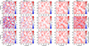 |
Fig. 5. Same as Figure 4 for the LOS velocity. |
| In the text | |
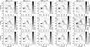 |
Fig. 6. Same as Figure 4 for the magnetic field strength. |
| In the text | |
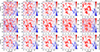 |
Fig. 7. Same as Figure 4 for the magnetic field inclination. |
| In the text | |
|
Fig. 8. Average differences between the input and the inferred atmosphere at different optical depths. From left to right, we show the differences in temperature, LOS velocity, magnetic field strength, and inclination. Colours correspond to the LTE case (blue) and NLTE assumption (red). Error bars display the standard deviation of the difference over the selected FOV at each optical depth. |
| In the text | |
Current usage metrics show cumulative count of Article Views (full-text article views including HTML views, PDF and ePub downloads, according to the available data) and Abstracts Views on Vision4Press platform.
Data correspond to usage on the plateform after 2015. The current usage metrics is available 48-96 hours after online publication and is updated daily on week days.
Initial download of the metrics may take a while.