| Issue |
A&A
Volume 659, March 2022
|
|
|---|---|---|
| Article Number | A117 | |
| Number of page(s) | 11 | |
| Section | Interstellar and circumstellar matter | |
| DOI | https://doi.org/10.1051/0004-6361/202142502 | |
| Published online | 15 March 2022 | |
X-ray irradiation of the stellar wind in HMXBs with B supergiants: Implications for ULXs
1
Ústav teoretické fyziky a astrofyziky, Přírodovědecká fakulta, Masarykova univerzita,
611 37
Brno,
Czech Republic
e-mail: krticka@physics.muni.cz
2
Astronomický ústav, Akademie věd České republiky,
251 65
Ondřejov,
Czech Republic
Received:
21
October
2021
Accepted:
9
February
2022
Wind-fed high-mass X-ray binaries are powered by accretion of the radiatively driven wind of the luminous component on the compact star. Accretion-generated X-rays alter the ionization state of the wind. Because higher ionization states drive the wind less effectively, X-ray ionization may brake acceleration of the wind. This causes a decrease in the wind terminal velocity and mass flux in the direction toward the X-ray source. Here we study the effect of X-ray ionization on the stellar wind of B supergiants. We determine the binary parameters for which the X-ray irradiation significantly influences the stellar wind. This can be conveniently studied in diagrams that plot the optical depth parameter versus the X-ray luminosity. For low optical depths or for high X-ray luminosities, X-ray ionization leads to a disruption in the wind aimed toward the X-ray source. Observational parameters of high-mass X-ray binaries with B-supergiant components appear outside the wind disruption zone. The X-ray feedback determines the resulting X-ray luminosity. We recognize two states with a different level of feedback. For low X-ray luminosities, ionization is weak, and the wind is not disrupted by X-rays and flows at large velocities, consequently the accretion rate is relatively low. On the other hand, for high X-ray luminosities, the X-ray ionization disrupts the flow braking the acceleration, the wind velocity is low, and the accretion rate becomes high. These effects determine the X-ray luminosity of individual binaries. Accounting for the X-ray feedback, estimated X-ray luminosities reasonably agree with observational values. We study the effect of small-scale wind inhomogeneities (clumping), showing that clumping weakens the effect of X-ray ionization by increasing recombination and the mass-loss rate. This effect is particularly important in the region of the so-called bistability jump. We show that ultraluminous X-ray binaries with LX ≲ 1040 erg s−1 may be powered by accretion of a B-supergiant wind on a massive black hole.
Key words: X-rays: binaries / stars: winds, outflows / stars: mass-loss / stars: early-type / stars: massive / hydrodynamics
© ESO 2022
1 Introduction
High-mass X-ray binaries (HMXBs) harbor a luminous massive star accompanied by a degenerate object, either a neutron star or a black hole. In a class of these binaries, the compact companion sails through the wind, which blows from the massive star, powering the X-ray emission via wind accretion (Davidson & Ostriker 1973; Lamers et al. 1976; Kretschmar et al. 2021).
Winds of hot stars are driven by light absorption and scattering in lines of heavy elements such as carbon, silicon, and iron (Lucy & Solomon 1970; Castor et al. 1975; Pauldrach et al. 1986). The strength of the wind is typically characterized by its mass-loss rate and terminal velocity. The mass-loss rate is defined as an amount of mass lost by the star per unit of time and the terminal velocity is a limiting wind velocity at large distances from the star. These parameters mostly determine the influence of the wind on the stellar evolution and circumstellar medium and can be estimated either from observations or theory.
The radiative force depends on the ionization state of the wind. Consequently, the X-ray irradiation may change the ionization balance and significantly alter the structure of the stellar wind. Because ions with a higher charge have effectively a lower number of levels and their resonance lines are outside the flux maximum, the X-ray irradiation weakens the radiative force. In HMXBs, this leads to a reduction in the terminal velocity and possibly also in the mass flux of the wind in a relatively narrow cone that faces the compact companion (Hatchett & McCray 1977; Fransson & Fabian 1980; Krtička et al. 2012).
The effect of X-ray irradiation provides important feedback for the wind structure. The amount of accreted matter and therefore also the X-ray luminosity is linearly proportional to the mass-loss rate, but inversely proportional to about the fourth power of wind velocity. Therefore, a decrease in the wind terminal velocity due to the X-ray irradiation significantly increases X-ray emission (Ho & Arons 1987; Krtička et al. 2018; Sander et al. 2018).
Such feedback might be especially important for ultraluminous X-ray sources (ULXs). These objects have X-ray luminosities higher than would correspond to the Eddington limit of a typical stellar black hole (Atapin 2018). Therefore, they were suspected to host intermediate mass black holes. While this still may be true for many of these sources, the detection of X-ray pulsations in some of the ULXs (Bachetti et al. 2014; Fürst et al. 2016) indicates that at least some of these sources may be powered by accretion on a neutron star. The strong influence of X-rays on the wind terminal velocity combined with high wind mass-loss rates could provide an explanation for the enormous X-ray luminosity of these objects.
While the X-ray irradiation has been systematically studied in HMXBs with O star primaries, such studies in the B star domain are only scarce (e.g., Sander et al. 2018). However, the domain of B supergiants is particularly interesting for HMXBs due to the bistability jump in mass-loss rates and terminal velocities, which can particularly boost the X-ray luminosity (Vink 2018). Therefore, here, we provide a grid of hot star wind models of B supergiants with X-ray irradiation focusing on the importance of the bistability jump and its relevance to ULXs.
2 Wind models
2.1 Global models without X-ray irradiation
Wind modeling was based on the grid of B-supergiant METUJE models described in detail by Krtička et al. (2021). Our models were calculated assuming a spherically symmetric and stationary stellar wind. The models self-consistently solve the same equations inthe photosphere and in the wind, which enables a smooth transition from the photosphere to the wind (global models). The radiative transfer was solved in the comoving frame (CMF; Mihalas et al. 1975). The atomic level occupation numbers were determined from the kinetic equilibrium equations (abbreviated as NLTE, Hubeny & Mihalas 2015, Chap. 9) with radiative bound-free terms calculated from the CMF radiative field and radiative bound-bound terms with the Sobolev approximation (Klein & Castor 1978). Atomic data for the solution of kinetic equilibrium equations were adopted mostly from the TLUSTY models (Lanz & Hubeny 2007) with additional updates from the Opacity and Iron Project data (Seaton et al. 1992; Hummer et al. 1993). We assumed a solar chemical composition after Asplund et al. (2009). The wind density, velocity, and temperature were derived from the continuity equation, the equation of motion with a radiative force due to continuum and line transitions, and the equation for energy (see Kubát 1996; Kubát et al. 1999, for details). We used the TLUSTY plane-parallel static model atmospheres (Lanz & Hubeny 2003, 2007) to derive the initial estimate of the photospheric structure.
The models were calculated for a grid of effective temperatures Teff = 15 000−25 000 K, assuming fixed luminosity L (and stellar mass M). The list of adopted parameters given in Table 1 was further supplemented by corresponding stellar radii R* and predicted mass-loss rates Ṁ. The predicted mass-loss rate of the model 150–60 is about five times higher than for the models with higher effective temperatures. This is a consequence of the so-called bistability effect (Pauldrach & Puls 1990). This effect is caused by the recombination of iron from Fe IV to Fe III, which accelerates wind more efficiently (Vink et al. 1999; Krtička et al. 2021).
Hot star winds show a small-scale structure which most likely originates due to the line-driven wind instability (Owocki et al. 1988; Feldmeier & Thomas 2017; Sundqvist et al. 2018). The inhomogeneities, also referred to as clumping, soften the influence of X-ray irradiation due to enhanced recombination (Oskinova et al. 2012; Krtička et al. 2018). To understand the influence of clumping, we additionally calculated a set of models that account for small-scale inhomogeneities (described in Krtička et al. 2018). We assumed that the stellar wind consists of homogeneous, optically thin overdensities (clumps) immersed invoid interclump space. We adopted a smooth velocity profile (describing the mean flow) for our modeling because the numerical simulations of line-driven wind instability predict that overdensities move at a velocity corresponding to a stationarywind solution (Feldmeier et al. 1997; Owocki & Puls 1999; Runacres & Owocki 2002) and that they do not directly influence the mass-loss rate. However, the line driving force in these numerical simulations is calculated using fixed line force parameters, that is different from what we used in our calculations. Consequently, these simulations do not account for the influence of overdensities on the level populations, which is what shall be included using our NLTE models. Therefore, within our assumptions, clumping affects just free-bound and free-free processes whose rates scale with the square of the density (see Krtička et al. 2018, for details). This is also a standard approach for spectral analysis of clumped winds (Hamann & Koesterke 1998; Hillier & Miller 1999; Puls et al. 2006).
The models with clumping are parameterized by a clumping factor  , where the angle brackets denote the average over volume. The clumping factor describes the density of the clump relatively to the mean density. We adopted radial clumping stratification motivated by empirical studies (Najarro et al. 2009; Bouret et al. 2012)
 (1)
(1)
which grows from unity in the photosphere (this is what corresponds to a smooth wind) to C1 for velocities larger than C2. We adopted the same values as in Krtička et al. (2021), that is C1 = 10, which is close to the mean value for which the empirical Hα mass-loss rates of B supergiants agree with observations (Krtička et al. 2021) and C2 = 100 km s−1, which is a typical value derived in the observational study of Najarro et al. (2009). In the formula for the radial clumping stratification Eq. (1), we inserted the fit ṽ (r) of the velocity of the smooth wind model (Cc = 1) via a modified polynomial form from Krtička & Kubát (2011) of
 (2)
(2)
where vi and γ are parameters of the fit given in Table 2 from Krtička et al. (2021).
The mass-loss rates predicted from models with clumping are given in the last column of Table 1. Clumping causes stronger recombination, which lowers the ionization state of atoms. Since lower ionization states typically accelerate the wind more effectively, clumping leads to a higher mass-loss rate (Muijres et al. 2011; Krtička et al. 2018). This effect is the strongest for the model 200-60, where the clumping causes an earlier onset for the bistability effect.
2.2 Inclusion of X-ray irradiation into NLTE models
The presence of an external source of X-ray radiation breaks the large-scale spherical symmetry of the stellar wind. The flow is disrupted by the gravity of the compact object and the accretion wake trailing the compact companion forms (Blondin et al. 1990; Manousakis & Walter 2015). Moreover, as a result of the weakening of the radiative force by X-rays, an ionization wake may form (Fransson & Fabian 1980; Feldmeier et al. 1996). On small scales, accretion of clumped wind contributes to X-ray variability (Oskinova et al. 2012; Bozzo et al. 2016; El Mellah et al. 2018).
Self-consistent modeling of such time-dependent phenomena requires multidimensional hydrodynamical simulations. However, coupling these simulations with a solution for the radiative transfer equation together with determination of atomic level population (i.e., the NLTE problem) is computationally prohibitive, and no such models are currently available. To make the problem tractable, we solved the stationary hydrodynamical equations assuming that the derived solution describes properties of the mean flow. We only accounted for the radial motion of the fluid, which is expected to be dominant in most cases. These approximations allow us to understand the influence of X-rays on the radiative force using 1D models, while the detailed 3D structure of the flow should be derived from hydrodynamical simulations. A similar approach was also used by other authors (Sander et al. 2018).
Similarly to Krtička et al. (2018), the influence of the compact secondary is only taken into account by the inclusion of external X-ray irradiation. We assume a point irradiating source located at the distance d from a given point in the wind, in which case the term
 (3)
(3)
has to be added to the mean radiation intensity Jν. Here,  is the monochromatic X-ray irradiation luminosity, whose frequency dependence is approximated by the power law
  for energies from 0.5 to 20 keV with a power law index Γ = 1. The monochromatic X-ray irradiation luminosity is normalized by the total X-ray luminosity,
  , which enters our models as a free parameter. A second free parameter of our models is the binary separation D, which is the distance between stellar centers (see Fig. 2 in Krtička et al. 2018). The binary separation enters the expression for the distance of a given point from the compact companion. Finally, τν (r) is the frequency-dependent optical depth between the given point in the wind and the compact companion,
 (4)
(4)
where κν is the X-ray mass-absorption coefficient.
Equation (3) allows one to calculate wind models for different inclinations with respect to the binary axis. Such models show that the influence of the X-ray irradiation is largest for zero inclination, that is, along the ray connecting stellar centers (Krtička et al. 2012). Therefore, we calculated wind models only along the direction of the binary axis.
To avoid possible problems with the convergence of the models, we did not use the density and opacity from the actual model in Eq. (4). Instead, we used the following analytical formula:
 (5)
(5)
Here vkink is the velocity of the kink that appears in the models with strong irradiation (otherwise we put vkink →∞),  is the fit from Eq. (2) of the wind velocity derived from the models without X-ray irradiation, and
  is the radially averaged mass-absorption coefficient given by1
 (6)
(6)
where λ is the value of the wavelength in units of Å. The parameters λ1, a0, a1, b1, a2, and b2 given in Table 2 were determined by fitting the mass-absorption coefficient of the models without X-ray irradiation averaged over radii 1.5 R*−5 R*. From Table 2 it follows that the parameters of the fit do not significantly vary with clumping in most cases; consequently, clumping does not strongly alter the opacity in the X-ray energy domain (Carneiro et al. 2016; Krtička et al. 2018).
To avoid numerical instabilities and problems with the CMF radiative force solution in the presence of a nonmonotonic velocity law, we used the photospheric flux to calculate the radiative force and applied a Sobolev line force corrected for CMF radiative transfer (see Krtička et al. 2012). This approach slightly shifts the stellar radius, which corresponds to the lower boundary of our models, affecting the velocity law used to determine clumping stratification. To compensate for this, we selected γ in Eq. (2) in such a way that it leads to the same mass-loss rate as calculated by Krtička et al. (2021) for global models with clumping (these mass-loss rates are also given in Table 1).
3 Influence of the X-ray irradiation on the wind structure of B supergiants
X-ray irradiation leads to stronger ionization, which means that the fraction of ions with higher ionization energies becomes higher. For weak X-ray irradiation, this leads to a slight increase in the radiative force because new states that contribute to the radiative force appear and ions with lower ionization energies remain nearly unaffected. However, strong X-ray irradiation depopulates ions with lower ionization energies, which are significant contributors to the radiative force. This leads to a decrease in the radiative force (Krtička et al. 2018; Sander et al. 2018).
The above mentioned influence of X-ray irradiation is proportional to the irradiating luminosity, which is inversely proportional to the electron number density n as a result of an increase in the recombination with density, and inversely proportional to the square of distance from the X-ray source due to the spatial dilution of radiation. This motivates the basic form of the ionization parameter introduced by Tarter et al. (1969, see also Hatchett & McCray 1977). Moreover, the recombination is stronger in clumped media (Oskinova et al. 2012) and a part of the emitted X-rays may be absorbed in the intervening media (Karino 2014). Consequently, Krtička et al. (2018) introduced the ionization parameter as
 (7)
(7)
From this equation, it follows that the X-ray irradiation is especially important in a close neighborhood of the X-ray source and for the X-ray sources with higher luminosity.
The influence of the X-ray irradiation is demonstrated in Fig. 1, where we plotted radial variations of velocity of the model 150-60 without clumping for two luminosities of the external irradiating source and different locations of the source. Close to the star, the wind density is very high and the dependence on the optical depth dominates Eq. (7). Consequently, the ionization parameter is very low and the wind velocity corresponds to the case without X-ray irradiation. This changes in a close proximity of the X-ray source, where the optical depth becomes lower than one and other dependencies prevail in Eq. (7).
Strong X-ray ionization leads to a decrease in the radiative force, which is unable to accelerate the wind any more and to sustain the flow with monotonically increasing velocity at a given mass flux (Feldmeier & Shlosman 2000; Feldmeier et al. 2008). As a consequence, a kink in the radial dependence of velocity appears (see Fig. 1). The position of the kink therefore marks the region with a strong interaction of irradiating X-rays with the supergiant wind. Figure 1 shows that with decreasing binary separation, the position of the kink moves toward the star reflecting a stronger influence of X-rays on the flow. The models with the shortest binary separations are not extended up to large radii due to convergence problems that appear when the velocity kink is located at low speeds. Moreover, the wind may not reach the companion in such a case and it may fall back to the star.
When the X-rays start to influence the structure of the flow close to the point where the wind velocity is equal to the Abbott speed (of the radiative acoustic waves, Abbott 1980) and where the wind mass-loss rate is determined, the wind becomes inhibited by X-rays leading to a significant decrease in the wind mass flux (Krtička et al. 2018). Therefore, for a given X-ray luminosity, there is a minimum binary separation that does not lead to the wind inhibition. Wind inhibition appears for binary separations that are lower than those plotted in Fig. 1.
With higher irradiating luminosity, the influence of X-rays becomes stronger (Fig. 1, right panel) and the position of the kink moves toward the star. Therefore, with increasing X-ray luminosity, the minimum binary separation for which the wind is not inhibited increases. The kink in v(r) appears even for extreme binary separations of about a hundred stellar radii for an X-ray luminosity corresponding to the ULX regime (LX = 1041 erg s−1).
Clumping reduces the influence of X-rays (Fig. 2). With clumping, recombination becomes more efficient, and therefore a closer or stronger X-ray source is needed to disrupt the wind. Moreover, clumping leads to an increase in the mass-loss rate, which further weakens the effect of X-rays. The reduction of the influence of X-rays due to clumping appears in all model stars studied here and becomes especially apparent for the model 150-60 with the highest mass-loss rate. Here, only a model for a very close X-ray source of D = 200 R⊙ and extreme X-ray irradiation with LX = 1041 erg s−1 leads to wind inhibition.
We additionally calculated a small set of models with a modified index of spectral energy distribution of irradiating X-rays Γ = 1.5 to test the influence of this parameter. The results showed that the radius where the kink of the velocity profile appears is typically shifted by less than a few percent. Therefore the slope of irradiating X-ray emission does not significantly influence the final results.
We have described the influence of X-rays on the wind terminal velocity and mass-loss rate using similar parametric relations as Krtička et al. (2018). The terminal velocity in the direction of the companion as a function of X-ray luminosity and binary separation was expressed for the models with clumping using modified Eq. (14) from Krtička et al. (2018) as
 (8)
(8)
Here L36 = 1036 erg s−1 and the values of fit parameters v∞,0, β1, β2, Δv∞, d1, d2, and d3, which were determined from the fit of the results from our models, are given in Table 3. The first term in Eq. (8) describes the increase in the terminal velocity with a decreasing influence of X-rays, while the exponential term accounts for a peak in the terminal velocity for medium irradiation. The dependence of the predicted mass fluxes on the X-ray luminosity and binary separation, which roughly describes the effect of wind inhibition, can be approximated as
![\begin{equation*}\dot m({L_{\textrm{X}}},D)=\frac{\dot M({L_{\textrm{X}}},D)}{4\pi R_{\ast}^2}=\frac{\dot M_0}{4\pi R_{\ast}^2}\left[{1-\exp\left({-\frac{\left({D/R_*-1}\right)^2}{s_1({L_{\textrm{X}}}/L_{36})^{s_2}}}\right)}\right].\end{equation*}](/articles/aa/full_html/2022/03/aa42502-21/aa42502-21-eq15.png) (9)
(9)
Here Ṁ0, s1, and s2 are parameters, which were determined by fitting predicted mass-loss rates (see Table 4). We note that the constant s1 is dimensionless here, while in Krtička et al. (2018, Eq. (15)), it is expressed in units of  . The region of parameters where Eq. (9) predicts
  corresponds to wind inhibition. X-rays disrupt the flow only in parts of the supergiant irradiated by the compact companion (Krtička et al. 2012) with a peak at the line connecting stellar centers; therefore, the total mass-loss rate, which can be derived by integration of mass fluxes over the supergiant surface, is only slightly affected by irradiation.
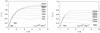 |
Fig. 1 Radial variations of velocity in the model 150-60 without clumping with the total X-ray luminosity LX = 1037 erg s−1 (left panel) and LX = 1041 erg s−1 (right panel). Individual curves are labeled by a binary separation D in units of R⊙. |
4 Test against observations: Diagrams of the X-ray luminosity versus the optical depth parameter
In optically thick media, the influence of X-ray irradiation, which can be quantified by the ionization parameter Eq. (7), mostly depends on the optical depth between a given point in the wind and the X-ray source. In inserting the density and opacity from Eq. (5) into the expression for the optical depth Eq. (4) assuming that the wind has reached the terminal velocity, the expression can be integrated to give  . This motivated us to introduce the optical depth parameter (Krtička et al. 2015, Eq. (3))
 (10)
(10)
which is proportional to the radial optical depth between the stellar surface and the X-ray source.
The diagrams that display the X-ray luminosity versus the optical depth parameter were proven to be effective in separating domains according to the type of influence that X-rays have on the wind (Krtička et al. 2018). These diagrams are plotted for studied B supergiants in Figs. 3 and 4 for the models without clumping and with clumping, respectively. From the diagrams, it follows that the stellar wind is strongly influenced by X-ray irradiation, either for high X-ray luminosities or for low X-ray optical depth parameters. The latter in fact implies X-ray sources that are very close to the supergiant. There is a zone where the X-ray irradiation becomes so strong that it is able to inhibit the wind. No wind-fed X-ray binary should exist in the zone of wind inhibition.
To test this prediction, we collected parameters of HMXBs with B-supergiant primaries from the literature (see Table 5) and placed these binary systems into X-ray luminosity versus optical depth diagrams in Fig. 3. Contrary to our prediction, a significant fraction of binaries lies in the region where we expect wind inhibition.
In more realistic models that account for clumping, the mass-loss rate is higher and the recombination becomes stronger. Therefore, the zone of the wind inhibition recedes in the X-ray luminosity versus optical depth diagram (see Fig. 4). This alleviates the problem of binaries that appear in the region of wind inhibition. Moreover, a significant fraction of binary systems appears close to the inhibition region boundary, which is what indicates that their X-ray luminosities may be self-regulated (Krtička et al. 2018).
Out of the studied models, the coolest one (150-60) is least influenced by X-rays. This is caused by the combination of its highest mass-loss rate, slow velocity leading to a denser wind (Vink 2018), higher X-ray opacity due to neutral helium, and generally weaker ionization with no irradiation.
Many of the HMXB primaries listed in Table 5 have radii comparable to the orbital separation. If they evolve toward red parts of the Hertzsprung-Russell diagram, then their radius quickly approaches the binary separation, as inferred from evolutionarymodels of Ekström et al. (2012). This puts the purely wind accretion commencing Roche lobe overflow phase (Tutukov & Yungelson 1973) to its end. This offers an explanation for the lack of HMXBs with late-supergiant primaries (Liu et al. 2006)provided that the binary separation does not significantly expand over the course of evolution (Schrøder et al. 2021).
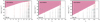 |
Fig. 3 Diagrams of the X-ray luminosity versus the optical depth parameter in Eq. (10) for wind models without clumping of individual B supergiants with parameters given in Table 1. Individual symbols correspond to models with different LX and D. Different symbols distinguish between various effects of X-ray ionization on the wind: black plus symbols denote models with a negligible influence of X-ray irradiation and red crosses denote models where the X-ray irradiation reduces the terminal velocity. The antique pink area marks the parameter region where the wind is inhibited by X-rays. The positions of B supergiant components of HMXBs from Table 5 are overplotted (green filled circles). |
5 Predicting the X-ray luminosity
The X-ray emission of wind-powered HMXBs originates due to the release of gravitational potential energy during accretion of the stellar wind (Davidson & Ostriker 1973; Lamers et al. 1976). The resulting X-ray luminosity is affected by processes acting on very different spatial scales, from the scales comparable to binary separation (Manousakis & Walter 2015; Xu & Stone 2019), at which the global properties of the flow are determined, across the magnetospheric radius of the neutron star(Shakura et al. 2012; Bozzo et al. 2016), which determines the way in which the material enters the magnetosphere (if there is a magnetosphere), down to scales comparable to a neutron star radius or Schwarzschild radius.
The accretion rate and associated accretion luminosity can be determined within the approximate Bondi-Hoyle-Lyttleton theory (Hoyle & Lyttleton 1941; Bondi & Hoyle 1944), which despite its numerous simplifications provides reasonable estimates for the accretion rate in many circumstances (Xu & Stone 2019). With MX and RX denoting the mass and radius of an accreting object, respectively, and v being its velocity relative to the wind flow, the Bondi-Hoyle-Lyttleton accretion luminosity is (Lamers et al. 1976)
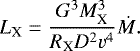 (11)
(11)
Here G is the gravitational constant. This equation gives the maximum X-ray luminosity, which assumes a maximum efficiency for the Bondi-Hoyle-Lyttleton accretion mechanism (e.g., Martínez-Núñez et al. 2017; Sidoli et al. 2021). The relative velocity can be estimated using the orbital velocity of the compact component vorb and the wind velocity at the distance D of the compact component, vwind = v(D), as
 (12)
(12)
For simplicity, we inserted vwind = v∞.
For the given stellar and binary parameters, Eq. (11) provides the X-ray luminosity due to wind accretion as a function of the wind velocity and mass flux. However, these wind parameters are modified by X-ray irradiation (Eqs. (8) and (9)). Consequently, Eq. (11) predicts the accretion X-ray luminosity as a function of X-ray irradiation. This function is plotted in Fig. 5 for individual model stars and for different orbital separations. For the plots we assumed generic neutron star parameters MX = 1.4 M⊙ and RX = 10 km.
For weak X-ray irradiation, the wind terminal velocity and the mass flux remain unaffected. Wind flows at large velocities; therefore, only a small fraction of the wind is collected by the compact companion, and consequently the resulting X-ray emission is weak (Fig. 5). For stronger X-ray irradiation, the terminal velocity decreases; as a result, the compact companion accretes more wind and the X-ray emission becomes much stronger (Ho & Arons 1987; Karino 2014). When the wind velocity is negligible with respect to the orbital velocity,  from Eq. (12), the X-ray luminosity reaches its maximum value, which is
  from Eq. (11), that is to say it is a factor of
  lower than one would get from a complete accretion of the stellar wind. We note that the maximum X-ray luminosity does not depend on the binary separation; therefore, even binaries with relatively large separations may have strong X-ray luminosities. However, even the mass flux decreases for very large X-ray luminosities. This leads to inhibition of the wind and X-ray emission (Fig. 5). For lower binary separations, the influence of X-rays becomes stronger; therefore, the plots shift to the left and their maxima shift to lower values of LX in Fig. 5.
In a stationary state, the irradiation X-ray luminosity is equal to the accretion luminosity (Karino 2014; Krtička et al. 2018; Bozzo et al. 2021). Consequently, Eq. (11) can be regarded as an implicit equation for LX. Individual solutions of this equation correspond to the points where the curves of X-ray luminosity intersect with the one-to-one relation in Fig. 5. For large binary separations, there is just one root of Eq. (11) corresponding to low X-ray luminosity and a weak influence of X-rays. For medium separation, there may be up to three solutions corresponding to different X-ray luminosities and different strengths of the influence of X-rays. The solutions with low X-ray luminosities disappear for small binary separations and only a solution with a high luminosity and strong influence of X-rays remains.
Not all of discussed solutions are stable. If the slope of the function is steeper than the slope of the one-to-one relation, then a small perturbation leads to runaway from the initial solution (Krtička et al. 2018). From the lower plot of Fig. 5, it follows that this happens for the middle solutions. Therefore, only solutions with the largest and the lowest X-ray luminosities are stable.
We applied Eq. (11) to determine the X-ray luminosities of HMXBs with B-supergiant components listed in Table 5. We inserted their stellar and binary parameters and accounted for the influence of X-rays on their terminal velocities (via Eq. (8)). Most stars show a solution with a strong decrease in the wind velocity and high X-ray luminosity on the order of 1036 erg s−1. This value corresponds to typical values found from observations (column LX in Table 5).
A class of HMXBs is characterized with relatively low quiescent X-ray luminosities 1032 −1033 erg s−1 and sporadic outbursts reaching X-ray luminosities on the order of 1036 erg s−1. These binaries are called supergiant fast X-ray transients (SFXTs) and objects that belong to this group are marked in Table 5 by a superscript c. Karino (2014) and Krtička et al. (2018) propose that low quiescent X-ray luminosities of SFXTs correspond to low-luminosity solutions of Eq. (11), for which the wind is not significantly affected by X-rays. Bozzo et al. (2021) argue that the transitions from the low luminosity state to the high luminosity state and back are modulated by changing the binary separation on highly eccentric orbits. Here we additionally demonstrate a bimodality of wind solutions in B-supergiant HMXBs, which appears for particular system parameters due to stronger sensitivity of the wind velocity on X-ray luminosity (higher β1 and β2 in Eq. (8)), and which is absent in O-supergiant HMXBs (Krtička et al. 2018).
In addition to the solutions with a high luminosity, some of the SFXTs in Table 5 also have low-luminosity solutions. This might be an explanation for their SFXT properties, but the distance variations during orbital motion may also be important, as suggested by Bozzo et al. (2021).
From Fig. 5, it follows that only binaries with a relatively small separation D ≲ 200 R⊙ are strong X-ray sources with X-ray luminosities on the order of 1036 erg s−1. This means that there can be a large population of X-ray quiet binaries with degenerate companions and X-ray luminosities on the order of 1033 erg s−1. This is a typical X-ray luminosity of single OB stars (Antokhin et al. 2008); therefore, these binaries may be hidden among B supergiants without compact companions.
It is possible to combine our sample of B-supergiant HMXBs with O-star HMXBs from Krtička et al. (2018) and to solveEq. (11) to derive an estimate for the X-ray luminosity of these binaries. While this approach provides a good estimate for the X-ray luminosity of stars with high observed luminosities LX > 1036 erg s−1, predictions for binaries with low X-ray luminosities are typically overestimated. This perhaps happens because the curve predicted by Eq. (11) is closely aligned with the one-to-one relation and; therefore, a small change in the binary parameters may cause alarge change in the predicted X-ray luminosity.
To alleviate this problem, we inserted the wind terminal velocity determined via Eq. (8) using observed X-ray luminosity into Eq. (11). The predicted X-ray luminosities estimated in this way nicely agree with observed values (see Fig. 6). A good agreement between observed and estimated X-ray luminosities results from a decrease in the wind velocity due to X-ray irradiation (Sander et al. 2018; Krtička et al. 2018). Without taking the influence of X-rays on the wind velocity into account, the estimated values of LX are by one to two orders of magnitude lower.
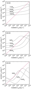 |
Fig. 5 X-ray luminosity generated by wind accretion as a function of X-ray irradiation after Eq. (11) accounting for the dependence of the terminal velocity and the mass flux on X-ray irradiation via Eqs. (8) and (9). The figure was plotted for individual model stars from Table 1 and for different binary separations labeled in the plots. The pink line denotes the one-to-one relation. |
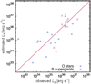 |
Fig. 6 X-ray luminosities of B-supergiant HMXBs (from Table 5) and O-star HMXBs (from the list of Krtička et al. 2018) estimated using Eqs. (11) and (12) inserting the wind terminal velocity derived from Eq. (8) calculated using observed X-ray luminosity. Plotted against observed X-ray luminosity. The pink line denotes the one-to-one relation. |
6 Implications for ULXs
Typical ULXs have X-ray luminosities in excess of 1039 erg s−1 (Swartz et al. 2004; Walton et al. 2011). Although the ULXs are believed to be powered mostly by Roche lobe overflow (Karino 2018; El Mellah et al. 2019), the wind accretion remains a viable option at least for some of these sources (Miller et al. 2014; Wiktorowicz et al. 2021).
From Fig. 5 it follows that the maximum X-ray luminosity stemming from the accretion of a B-supergiant wind on a neutron star is on the order of 1037 erg s−1. Therefore, a higher mass for the compact object is required to obtain luminosities in the ULX regime. In Fig. 7 we plotted the accretion X-ray luminosity as a function of the X-ray irradiation for the binaries where the compact companion is a black hole with a mass of 20 M⊙ instead of a neutron star. The value for the black-hole mass is motivated by an updated mass of Cygnus X-1 derived from radio interferometry (Miller-Jones et al. 2021). As a result of cubic dependence of the X-ray luminosity on the compact-companion mass, the resulting X-ray luminosities are by two to three orders of magnitude higher than those for a neutron star. For B supergiants below the bistability jump, the maximum possible X-ray luminosities correspond to the weaker end of ULX regime.
X-ray luminosities corresponding to a weak effect of X-ray irradiation are by several orders of magnitude lower (Fig. 7). Therefore, there might exist a population of quiet HMXBs with massive black holes as a central engine and X-ray luminosities on the order of 1035−1036 erg s−1.
Strong X-ray irradiation not only inhibits wind acceleration, but it may also affect the spectrum of B supergiants. To understand this effect, we included the X-ray irradiation in TLUSTY atmosphere models (Lanz & Hubeny 2003, 2007). The external irradiation is included as an outer boundary condition for a specific intensity,
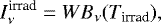 (13)
(13)
where  is a dilution factor, Rirrad is the effective radius of the irradiating body, and Bν(Tirrad) is Planck law at the temperature Tirrad. With
  , the dilution factor W is related to the X-ray luminosity and source distance as
 (14)
(14)
Taking the possible parameters of ULXs into account, we calculated two sets of atmosphere models with W = 10−11 and W = 10−13 and with Tirrad = 107 K.
Even for strong X-ray irradiation, the resulting spectra are nearly indistinguishable from the spectra without any irradiation (Fig. 8). Although the X-rays are able to heat the outer regions of the photosphere by several tens of thousands of Kelvin, only layers with a low Rosseland optical depth τross ≲ 10−3 are affected, and therefore the influence of X-ray irradiation on emergent optical spectrum is relatively weak. As a result, only a few absorption lines (e.g., He II 4686, 5412, and 6560 Å) become stronger in the irradiated spectra due to an increase in populations of excited levels of He II by incoming X-rays. There are additional lines in the infrared domain which show enhanced emission due to irradiation, for instance the He I 18 685 Å line. Irradiated spectra given in Fig. 8 correspond to the maximum irradiation in the surface region that directly faces the neutron star. Other regions receive less flux, and consequently the integrated effect is expected to be even lower.
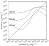 |
Fig. 7 X-ray luminosity generated by wind accretion on a 20 M⊙ black hole located at D = 300 R⊙ as a functionof X-ray irradiation after Eq. (11). Plotted for individual model stars from Table 1. The pinkline denotes the one-to-one relation. |
7 Conclusions
We studied the effect of X-ray irradiation on the stellar wind in HMXBs powered by the accretion of B-supergiant wind on its compact companion. We included an external X-ray source in our B-supergiant wind models. For each model star corresponding to B supergiants, we calculated a grid of models parameterized by the binary separation and external irradiation X-ray luminosity. We also calculated models with optically thin inhomogeneities (clumping).
It is well known that accretion-generated X-rays alter the ionization state of the wind. Higher ionization states, which appear due to X-ray ionization, drive the wind less effectively and, consequently, brake acceleration of the wind. This causes a decrease in the wind terminal velocity and, for strong X-ray irradiation, also a decrease in the mass flux in the direction of the companion. These effects are particularly important for short binary separations and high X-ray luminosities. The X-ray ionization can be partially compensated for by wind clumping, which increases recombination and mass-loss rates. The influence of clumping is particularly strong in the region of the bistability jump, where the mass-loss rate increases toward lower effective temperatures by a factor of a few as a result of iron recombination.
The strength of X-ray illumination can be conveniently demonstrated in the diagrams that plot (undisturbed) optical depth parameter versus the X-ray luminosity. There is a parameter region of high X-ray luminosities and low optical depth parameters in these diagrams, where the X-ray ionization leads to the disruption of the wind. Observational parameters of high-mass X-ray binaries with B supergiant components appear outside the zone of wind disruption, which is in agreement with clumped-wind model results. Moreover, a significant fraction of HMBXs appears close to the border of wind disruption indicating that their X-ray luminosities may be self-regulated.
The X-ray feedback determines the X-ray luminosity resulting from wind accretion. We recognized two states of feedback. For low X-ray luminosities, the X-ray ionization is weak, the wind is not disrupted by X-rays, it flows at large velocities, and consequently the accretion rate is relatively low. On the other hand, for high X-ray luminosities, the X-ray ionization disrupts the flow braking the acceleration of the flow facing the companion, the wind velocity is low, and the accretion rate becomes high. We demonstrated that these effects determine the X-ray luminosity of individual binaries. By accounting for wind inhibition by X-rays, the estimated X-ray luminosities are consistent with observational values. Moreover, the two states of X-ray feedback can explain the appearance of two types of X-ray binaries, classical supergiant X-ray binaries and fast X-ray transients.
In HMXBs with massive black hole components, the X-ray luminosities may exceed 1039 erg s−1 for B supergiants below the bistability jump. This shows that part of the ULXs may be powered by the accretion of B-supergiant wind. Despite the presence of a strong illuminating source, the optical spectrum of such supergiants is nearly indistinguishable from the spectrum of single B supergiants.
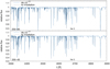 |
Fig. 8 Comparison of spectra of selected model stars with and without X-ray irradiation. |
Acknowledgements
Computational resources were supplied by the project “e-Infrastruktura CZ” (e-INFRA LM2018140) provided within the program Projects of Large Research, Development and Innovations Infrastructures. The Astronomical Institute Ondřejov is supported by a project RVO:67985815 of the Academy of Sciences of the Czech Republic.
References
- Abbott, D. C. 1980, ApJ, 242, 1183 [NASA ADS] [CrossRef] [Google Scholar]
- Antokhin, I. I., Rauw, G., Vreux, J.-M., van der Hucht, K. A., & Brown, J. C. 2008, A&A, 477, 593 [NASA ADS] [CrossRef] [EDP Sciences] [Google Scholar]
- Asplund, M., Grevesse, N., Sauval, A. J., & Scott, P. 2009, ARA&A, 47, 481 [NASA ADS] [CrossRef] [Google Scholar]
- Atapin, K. 2018, in Accretion Processes in Cosmic Sources - II, ed. F. Giovannelli (USA: PoS) [Google Scholar]
- Bachetti, M., Harrison, F. A., Walton, D. J., et al. 2014, Nature, 514, 202 [NASA ADS] [CrossRef] [Google Scholar]
- Blondin, J. M., Kallman, T. R., Fryxell, B. A., & Taam, R. E. 1990, ApJ, 356, 591 [Google Scholar]
- Bondi, H., & Hoyle, F. 1944, MNRAS, 104, 273 [Google Scholar]
- Bouret, J.-C., Hillier, D. J., Lanz, T., & Fullerton, A. W. 2012, A&A, 544, A67 [NASA ADS] [CrossRef] [EDP Sciences] [Google Scholar]
- Bozzo, E., Oskinova, L., Feldmeier, A., & Falanga, M. 2016, A&A, 589, A102 [NASA ADS] [CrossRef] [EDP Sciences] [Google Scholar]
- Bozzo, E., Ducci, L., & Falanga, M. 2021, MNRAS, 501, 2403 [NASA ADS] [CrossRef] [Google Scholar]
- Carneiro, L. P., Puls, J., Sundqvist, J. O., & Hoffmann, T. L. 2016, A&A, 590, A88 [NASA ADS] [CrossRef] [EDP Sciences] [Google Scholar]
- Castor, J. I., Abbott, D. C., & Klein, R. I. 1975, ApJ, 195, 157 [Google Scholar]
- Chakrabarty, D., Wang, Z., Juett, A. M., Lee, J. C., & Roche, P. 2002, ApJ, 573, 789 [NASA ADS] [CrossRef] [Google Scholar]
- Davidson, K., & Ostriker, J. P. 1973, ApJ, 179, 585 [NASA ADS] [CrossRef] [Google Scholar]
- Ekström, S., Georgy, C., Eggenberger, P., et al. 2012, A&A, 537, A146 [Google Scholar]
- El Mellah, I., Sundqvist, J. O., & Keppens, R. 2018, MNRAS, 475, 3240 [Google Scholar]
- El Mellah, I., Sundqvist, J. O., & Keppens, R. 2019, A&A, 622, L3 [NASA ADS] [CrossRef] [EDP Sciences] [Google Scholar]
- Farrell, S. A., Sood, R. K., O’Neill, P. M., & Dieters, S. 2008, MNRAS, 389, 608 [NASA ADS] [CrossRef] [Google Scholar]
- Feldmeier, A., & Shlosman, I. 2000, ApJ, 532, L125 [NASA ADS] [CrossRef] [Google Scholar]
- Feldmeier, A., & Thomas, T. 2017, MNRAS, 469, 3102 [NASA ADS] [CrossRef] [Google Scholar]
- Feldmeier, A., Anzer, U., Boerner, G., & Nagase, F. 1996, A&A, 311, 793 [NASA ADS] [Google Scholar]
- Feldmeier, A., Puls, J., & Pauldrach, A. W. A. 1997, A&A, 322, 878 [NASA ADS] [Google Scholar]
- Feldmeier, A., Rätzel, D., & Owocki, S. P. 2008, ApJ, 679, 704 [NASA ADS] [CrossRef] [Google Scholar]
- Ferrigno, C., Segreto, A., Mineo, T., Santangelo, A., & Staubert, R. 2008, A&A, 479, 533 [NASA ADS] [CrossRef] [EDP Sciences] [Google Scholar]
- Fransson, C., & Fabian, A. C. 1980, A&A, 87, 102 [NASA ADS] [Google Scholar]
- Fürst, F., Walton, D. J., Harrison, F. A., et al. 2016, ApJ, 831, L14 [Google Scholar]
- Giménez-García, A., Torrejón, J. M., Eikmann, W., et al. 2015, A&A, 576, A108 [NASA ADS] [CrossRef] [EDP Sciences] [Google Scholar]
- Giménez-García, A., Shenar, T., Torrejón, J. M., et al. 2016, A&A, 591, A26 [EDP Sciences] [Google Scholar]
- González-Galán, A., Negueruela, I., Castro, N., et al. 2014, A&A, 566, A131 [NASA ADS] [CrossRef] [EDP Sciences] [Google Scholar]
- Grunhut, J. H., Bolton, C. T., & McSwain, M. V. 2014, A&A, 563, A1 [NASA ADS] [CrossRef] [EDP Sciences] [Google Scholar]
- Hall, T. A., Finley, J. P., Corbet, R. H. D., & Thomas, R. C. 2000, ApJ, 536, 450 [NASA ADS] [CrossRef] [Google Scholar]
- Hamann, W. R., & Koesterke, L. 1998, A&A, 335, 1003 [Google Scholar]
- Hatchett, S., & McCray, R. 1977, ApJ, 211, 552 [NASA ADS] [CrossRef] [Google Scholar]
- Hill, A. B., Walter, R., Knigge, C., et al. 2005, A&A, 439, 255 [NASA ADS] [CrossRef] [EDP Sciences] [Google Scholar]
- Hillier, D. J., & Miller, D. L. 1999, ApJ, 519, 354 [Google Scholar]
- Ho, C., & Arons, J. 1987, ApJ, 316, 283 [NASA ADS] [CrossRef] [Google Scholar]
- Hoyle, F., & Lyttleton, R. A. 1941, MNRAS, 101, 227 [NASA ADS] [Google Scholar]
- Hubeny, I., & Mihalas, D. 2015, Theory of Stellar Atmospheres (Princeton: Princeton University Press) [Google Scholar]
- Hummer, D. G., Berrington, K. A., Eissner, W., et al. 1993, A&A, 279, 298 [NASA ADS] [Google Scholar]
- Hutchings, J. B., Crampton, D., Cowley, A. P., & Thompson, I. B. 1987, PASP, 99, 420 [NASA ADS] [CrossRef] [Google Scholar]
- Ikhsanov, N. R., & Finger, M. H. 2012, ApJ, 753, 1 [CrossRef] [Google Scholar]
- Kaper, L., van der Meer, A., & Najarro, F. 2006, A&A, 457, 595 [CrossRef] [EDP Sciences] [Google Scholar]
- Karino, S. 2014, PASJ, 66, 34 [NASA ADS] [Google Scholar]
- Karino, S. 2018, MNRAS, 474, 4564 [NASA ADS] [CrossRef] [Google Scholar]
- Klein, R. I., & Castor, J. I. 1978, ApJ, 220, 902 [NASA ADS] [CrossRef] [Google Scholar]
- Kretschmar, P., El Mellah, I., Martínez-Núñez, S., et al. 2021, A&A, 652, A95 [NASA ADS] [CrossRef] [EDP Sciences] [Google Scholar]
- Krtička, J., & Kubát, J. 2011, A&A, 534, A97 [NASA ADS] [CrossRef] [EDP Sciences] [Google Scholar]
- Krtička, J., Kubát, J., & Skalický, J. 2012, ApJ, 757, 162 [CrossRef] [Google Scholar]
- Krtička, J., Kubát, J., & Krtičková, I. 2015, A&A, 579, A111 [NASA ADS] [CrossRef] [EDP Sciences] [Google Scholar]
- Krtička, J., Kubát, J., & Krtičková, I. 2018, A&A, 620, A150 [NASA ADS] [CrossRef] [EDP Sciences] [Google Scholar]
- Krtička, J., Kubát, J., & Krtičková, I. 2021, A&A, 647, A28 [NASA ADS] [CrossRef] [EDP Sciences] [Google Scholar]
- Kubát, J. 1996, A&A, 305, 255 [NASA ADS] [Google Scholar]
- Kubát, J., Puls, J., & Pauldrach, A. W. A. 1999, A&A, 341, 587 [NASA ADS] [Google Scholar]
- Lamers, H. J. G. L. M., van den Heuvel, E. P. J., & Petterson, J. A. 1976, A&A, 49, 327 [NASA ADS] [Google Scholar]
- Lanz, T., & Hubeny, I. 2003, ApJS, 146, 417 [NASA ADS] [CrossRef] [Google Scholar]
- Lanz, T., & Hubeny, I. 2007, ApJS, 169, 83 [CrossRef] [Google Scholar]
- Liu, Q. Z., van Paradijs, J., & van den Heuvel, E. P. J. 2006, A&A, 455, 1165 [NASA ADS] [CrossRef] [EDP Sciences] [Google Scholar]
- Lorenzo, J., Negueruela, I., Castro, N., et al. 2014, A&A, 562, A18 [NASA ADS] [CrossRef] [EDP Sciences] [Google Scholar]
- Lucy, L. B., & Solomon, P. M. 1970, ApJ, 159, 879 [Google Scholar]
- Lutovinov, A. A., Revnivtsev, M. G., Tsygankov, S. S., & Krivonos, R. A. 2013, MNRAS, 431, 327 [Google Scholar]
- Manousakis, A., & Walter, R. 2015, A&A, 575, A58 [NASA ADS] [CrossRef] [EDP Sciences] [Google Scholar]
- Martínez-Núñez, S., Kretschmar, P., Bozzo, E., et al. 2017, Space Sci. Rev., 212, 59 [Google Scholar]
- Mason, A. B., Norton, A. J., Clark, J. S., Negueruela, I., & Roche, P. 2011, A&A, 532, A124 [NASA ADS] [CrossRef] [EDP Sciences] [Google Scholar]
- Mason, A. B., Clark, J. S., Norton, A. J., et al. 2012, MNRAS, 422, 199 [NASA ADS] [CrossRef] [Google Scholar]
- Mihalas, D., Kunasz, P. B., & Hummer, D. G. 1975, ApJ, 202, 465 [CrossRef] [Google Scholar]
- Miller, M. C., Farrell, S. A., & Maccarone, T. J. 2014, ApJ, 788, 116 [NASA ADS] [CrossRef] [Google Scholar]
- Miller-Jones, J. C. A., Bahramian, A., Orosz, J. A., et al. 2021, Science, 371, 1046 [Google Scholar]
- Muijres, L. E., de Koter, A., Vink, J. S., et al. 2011, A&A, 526, A32 [NASA ADS] [CrossRef] [EDP Sciences] [Google Scholar]
- Najarro, F., Figer, D. F., Hillier, D. J., Geballe, T. R., & Kudritzki, R. P. 2009, ApJ, 691, 1816 [NASA ADS] [CrossRef] [Google Scholar]
- Oskinova, L. M., Feldmeier, A., & Kretschmar, P. 2012, MNRAS, 421, 2820 [NASA ADS] [CrossRef] [Google Scholar]
- Owocki, S. P., & Puls, J. 1999, ApJ, 510, 355 [Google Scholar]
- Owocki, S. P., Castor, J. I., & Rybicki, G. B. 1988, ApJ, 335, 914 [NASA ADS] [CrossRef] [Google Scholar]
- Pauldrach, A. W. A., & Puls, J. 1990, A&A, 237, 409 [NASA ADS] [Google Scholar]
- Pauldrach, A., Puls, J., & Kudritzki, R. P. 1986, A&A, 164, 86 [NASA ADS] [Google Scholar]
- Puls, J., Markova, N., Scuderi, S., et al. 2006, A&A, 454, 625 [NASA ADS] [CrossRef] [EDP Sciences] [Google Scholar]
- Rahoui, F., & Chaty, S. 2008, A&A, 492, 163 [NASA ADS] [CrossRef] [EDP Sciences] [Google Scholar]
- Reig, P., Chakrabarty, D., Coe, M. J., et al. 1996, A&A, 311, 879 [NASA ADS] [Google Scholar]
- Romano, P., Sidoli, L., Mangano, V., Mereghetti, S., & Cusumano, G. 2007, A&A, 469, L5 [NASA ADS] [CrossRef] [EDP Sciences] [Google Scholar]
- Romano, P., Sidoli, L., Ducci, L., et al. 2010, MNRAS, 401, 1564 [NASA ADS] [CrossRef] [Google Scholar]
- Runacres, M. C., & Owocki, S. P. 2002, A&A, 381, 1015 [NASA ADS] [CrossRef] [EDP Sciences] [Google Scholar]
- Sander, A. A. C., Fürst, F., Kretschmar, P., et al. 2018, A&A, 610, A60 [NASA ADS] [CrossRef] [EDP Sciences] [Google Scholar]
- Schrøder, S. L., MacLeod, M., Ramirez-Ruiz, E., et al. 2021, ApJ, submitted [arXiv:2107.09675] [Google Scholar]
- Searle, S. C., Prinja, R. K., Massa, D., & Ryans, R. 2008, A&A, 481, 777 [NASA ADS] [CrossRef] [EDP Sciences] [Google Scholar]
- Seaton, M. J., Zeippen, C. J., Tully, J. A., et al. 1992, Rev. Mex. Astron. Astrofis., 23, 216 [Google Scholar]
- Servillat, M., Coleiro, A., Chaty, S., Rahoui, F., & Zurita Heras, J. A. 2014, ApJ, 797, 114 [NASA ADS] [CrossRef] [Google Scholar]
- Shakura, N., Postnov, K., Kochetkova, A., & Hjalmarsdotter, L. 2012, MNRAS, 420, 216 [Google Scholar]
- Sidoli, L., Postnov, K., Oskinova, L., et al. 2021, A&A, 654, A131 [NASA ADS] [CrossRef] [EDP Sciences] [Google Scholar]
- Sundqvist, J. O., Owocki, S. P., & Puls, J. 2018, A&A, 611, A17 [NASA ADS] [CrossRef] [EDP Sciences] [Google Scholar]
- Swartz, D. A., Ghosh, K. K., Tennant, A. F., & Wu, K. 2004, ApJS, 154, 519 [Google Scholar]
- Tarter, C. B., Tucker, W. H., & Salpeter, E. E. 1969, ApJ, 156, 943 [Google Scholar]
- Tutukov, A., & Yungelson, L. 1973, Nauchnye Informatsii, 27, 70 [NASA ADS] [Google Scholar]
- Vink, J. S. 2018, A&A, 619, A54 [NASA ADS] [CrossRef] [EDP Sciences] [Google Scholar]
- Vink, J. S., de Koter, A., & Lamers, H. J. G. L. M. 1999, A&A, 350, 181 [Google Scholar]
- Walter, R., Lutovinov, A. A., Bozzo, E., & Tsygankov, S. S. 2015, A&ARv, 23, 2 [Google Scholar]
- Walton, D. J., Roberts, T. P., Mateos, S., & Heard, V. 2011, MNRAS, 416, 1844 [Google Scholar]
- Watanabe, S., Sako, M., Ishida, M., et al. 2006, ApJ, 651, 421 [Google Scholar]
- Wiktorowicz, G., Lasota, J.-P., Belczynski, K., et al. 2021, ApJ, 918, 60 [CrossRef] [Google Scholar]
- Xu, W., & Stone, J. M. 2019, MNRAS, 488, 5162 [NASA ADS] [CrossRef] [Google Scholar]
All Tables
All Figures
|
Fig. 1 Radial variations of velocity in the model 150-60 without clumping with the total X-ray luminosity LX = 1037 erg s−1 (left panel) and LX = 1041 erg s−1 (right panel). Individual curves are labeled by a binary separation D in units of R⊙. |
| In the text | |
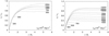 |
Fig. 2 Same as Fig. 1, but for clumping factor C1 = 10. |
| In the text | |
|
Fig. 3 Diagrams of the X-ray luminosity versus the optical depth parameter in Eq. (10) for wind models without clumping of individual B supergiants with parameters given in Table 1. Individual symbols correspond to models with different LX and D. Different symbols distinguish between various effects of X-ray ionization on the wind: black plus symbols denote models with a negligible influence of X-ray irradiation and red crosses denote models where the X-ray irradiation reduces the terminal velocity. The antique pink area marks the parameter region where the wind is inhibited by X-rays. The positions of B supergiant components of HMXBs from Table 5 are overplotted (green filled circles). |
| In the text | |
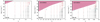 |
Fig. 4 As in Fig. 3, but for models with clumping. |
| In the text | |
|
Fig. 5 X-ray luminosity generated by wind accretion as a function of X-ray irradiation after Eq. (11) accounting for the dependence of the terminal velocity and the mass flux on X-ray irradiation via Eqs. (8) and (9). The figure was plotted for individual model stars from Table 1 and for different binary separations labeled in the plots. The pink line denotes the one-to-one relation. |
| In the text | |
|
Fig. 6 X-ray luminosities of B-supergiant HMXBs (from Table 5) and O-star HMXBs (from the list of Krtička et al. 2018) estimated using Eqs. (11) and (12) inserting the wind terminal velocity derived from Eq. (8) calculated using observed X-ray luminosity. Plotted against observed X-ray luminosity. The pink line denotes the one-to-one relation. |
| In the text | |
|
Fig. 7 X-ray luminosity generated by wind accretion on a 20 M⊙ black hole located at D = 300 R⊙ as a functionof X-ray irradiation after Eq. (11). Plotted for individual model stars from Table 1. The pinkline denotes the one-to-one relation. |
| In the text | |
|
Fig. 8 Comparison of spectra of selected model stars with and without X-ray irradiation. |
| In the text | |
Current usage metrics show cumulative count of Article Views (full-text article views including HTML views, PDF and ePub downloads, according to the available data) and Abstracts Views on Vision4Press platform.
Data correspond to usage on the plateform after 2015. The current usage metrics is available 48-96 hours after online publication and is updated daily on week days.
Initial download of the metrics may take a while.