| Issue |
A&A
Volume 659, March 2022
|
|
|---|---|---|
| Article Number | A89 | |
| Number of page(s) | 19 | |
| Section | Extragalactic astronomy | |
| DOI | https://doi.org/10.1051/0004-6361/202141568 | |
| Published online | 11 March 2022 | |
Aperture-corrected spectroscopic type Ia supernova host galaxy properties⋆
1
Institute of Space Sciences (ICE, CSIC), Campus UAB, Carrer de Can Magrans, s/n, 08193 Barcelona, Spain
e-mail: This email address is being protected from spambots. You need JavaScript enabled to view it.
2
Institut d’Estudis Espacials de Catalunya (IEEC), 08034 Barcelona, Spain
3
Univ. Lyon, Univ. Claude Bernard Lyon 1, CNRS, IP2I Lyon/IN2P3, IMR 5822, 69622 Villeurbanne, France
4
Département de Physique, de Génie Physique et d’Optique, Université Laval, and Centre de Recherche en Astrophysique du Québec (CRAQ), Québec, QC G1V 0A6, Canada
5
Instituto de Astrofísica de Andalucía – CSIC, Glorieta de la Astronomía s.n., 18008 Granada, Spain
6
CENTRA/COSTAR, Instituto Superior Técnico, Universidade de Lisboa, Av. Rovisco Pais 1, 1049-001 Lisboa, Portugal
7
Max-Planck-Institute for Astronomy, Königstuhl 17, 69117 Heidelberg, Germany
8
Department of Physics and Astronomy, University of Pennsylvania, Philadelphia, PA 19104, USA
9
Australian Astronomical Optics, Macquarie University, 105 Delhi Rd, North Ryde, NSW 2113, Australia
10
Department of Physics and Astronomy, Macquarie University, Sydney, NSW 2109, Australia
11
Macquarie University Research Centre for Astronomy, Astrophysics & Astrophotonics, Sydney, NSW 2109, Australia
12
ARC Centre of Excellence for All Sky Astrophysics in 3 Dimensions (ASTRO-3D), Sydney, Australia
13
Dpto. de Investigación Básica, CIEMAT, Avda. Complutense 40, 28040 Madrid, Spain
Received:
14
June
2021
Accepted:
4
December
2021
Abstract
We use type Ia supernova (SN Ia) data obtained by the Sloan Digital Sky Survey-II Supernova Survey (SDSS-II SNS) in combination with the publicly available SDSS DR16 fiber spectroscopy of supernova (SN) host galaxies to correlate SN Ia light-curve parameters and Hubble residuals with several host galaxy properties. Fixed-aperture fiber spectroscopy suffers from aperture effects: the fraction of the galaxy covered by the fiber varies depending on its projected size on the sky, and thus measured properties are not representative of the whole galaxy. The advent of integral field spectroscopy has provided a way to correct the missing light, by studying how these galaxy parameters change with the aperture size. Here we study how the standard SN host galaxy relations change once global host galaxy parameters are corrected for aperture effects. We recover previous trends on SN Hubble residuals with host galaxy properties, but we find that discarding objects with poor fiber coverage instead of correcting for aperture loss introduces biases into the sample that affect SN host galaxy relations. The net effect of applying the commonly used g-band fraction criterion is that intrinsically faint SNe Ia in high-mass galaxies are discarded, thus artificially increasing the height of the mass step by 0.02 mag and its significance. Current and next-generation fixed-aperture fiber-spectroscopy surveys, such as OzDES, DESI, or TiDES with 4MOST, that aim to study SN and galaxy correlations must consider, and correct for, these effects.
Key words: dark energy / galaxies: star formation / techniques: spectroscopic / supernovae: general / galaxies: abundances
Full Table D.1 is only available at the CDS via anonymous ftp to cdsarc.u-strasbg.fr (130.79.128.5) or via http://cdsarc.u-strasbg.fr/viz-bin/cat/J/A+A/659/A89
© ESO 2022
1. Introduction
The discovery of the accelerated expansion of the Universe was possible thanks to the use of type Ia supernovae (SNe Ia) as distance indicators (Riess et al. 1998; Perlmutter et al. 1999). Given their extreme brightness, SNe Ia can be detected even in very distant galaxies (z ≳ 1) from the ground with mid-size (∼4 m) telescopes. At optical wavelengths, they show a scatter of ∼2 mag in their peak brightness, but this can be standardized by accounting for empirical relations with the brightness decay rate (or light-curve width; Phillips 1993) and color at peak (Riess et al. 1996). Once standardized, the precision in the distance measurements is reduced down to 5–7% (Betoule et al. 2014; Brout et al. 2019).
Over the years, the accumulation of new observations has weighted down statistical errors, and the focus is now on the reduction of the systematic uncertainties. Such systematics can be reduced by improving the cadence of the observed light curves (Rose et al. 2020), the photometric calibration of the fitting and minimization routines, or by modifying the standardization method, either adding new parameters to the widely used Tripp expression (Tripp 1998) or exploring other, nonlinear approaches (Rubin et al. 2015; Mandel et al. 2022). There is also evidence that near-infrared (NIR) observations, which are naturally less affected by reddening, present very low scatter on their peak magnitudes even with no corrections, which turns them into almost natural standard candles (Dhawan et al. 2018; Burns et al. 2018). Also, other cosmological effects that impact measurements at high redshift (e.g., weak lensing; Smith et al. 2014) need to be accounted for to reduce the systematic uncertainty budget.
One of these sources of systematics is the different environments where SNe Ia occur. Given that the characterization of the near local vicinity is problematic for farther objects (see, for instance, Rigault et al. 2013, 2020; Jones et al. 2018; Kelsey et al. 2021), these efforts have been focused on measurements of the global properties of supernova (SN) host galaxies, such as morphology, mass, age, star-formation rate (SFR), or metallicity. Several correlations between SN properties and their environment have been reported so far: Hamuy et al. (1996) first found a correlation between SN Ia stretch and the Hubble type of its host, with late-type galaxies hosting observationally brighter events compared to early-type hosts. This morphological classification is related to other galactic properties, such as the SFR, age, or mass. Sullivan et al. (2006) showed that high-stretch events were found in systems with ongoing star formation, corresponding to the late-type galaxies. In terms of stellar population age, it was also found that galaxies that have younger mean ages host observationally brighter SNe (Hamuy et al. 1995, 2000. These correlations have also been confirmed in more recent works with larger SN samples by Gallagher et al. (2005), Gupta et al. (2011), Childress et al. (2013b), Rose et al. (2019), and Smith et al. (2020). The total mass of the galaxy has also been correlated to both the observed and the standardized SN brightness (Kelly et al. 2010; Sullivan et al. 2010), providing the base for the introduction of a new term in the standardization equation that accounts for a host environmental parameter (the γ mass term; Lampeitl et al. 2010). More recently, further efforts have been focused on studying this dependence at NIR wavelengths (Uddin et al. 2020; Ponder et al. 2021) and its relation with dust and the extinction law (Brout & Scolnic 2021; González-Gaitán et al. 2021).
Supernova host galaxy parameters are primarily obtained from photometric magnitudes. Obtaining imaging of SN host galaxies is relatively easy; it may be available from observations of the same rolling surveys, either before the SN or after when the SN is already undetected, or even from archival images. However, host galaxy parameters measured from photometry are less precise than when measured from spectroscopy since the whole spectral energy distribution and the properties of the galaxy are inferred from only a few photometric points. Although spectroscopy provides more precise information, it also presents some difficulties. Obtaining spectroscopy of SN host galaxies is difficult and far from common in SN surveys.
Problematically, the full extent of the galaxy is not usually covered by the fiber or slit, and galactic parameters measured from the spectra are representative only of the fraction of the area covered by the fiber or slit. To overcome this problem, one common approach followed in the literature is to scale the spectrum to match the integrated light of the galaxy. Although this helps with extensive properties, such as the stellar mass or the SFR, it still retains the assumption of extrapolating the properties of the area covered within the fiber or slit to the other regions of the galaxy (usually the outskirts), where intensive properties, such as metallicity, age, and extinction, are known to change either in terms of radial gradients or structurally (e.g., from arm to inter-arm; Sánchez et al. 2015; Sánchez-Menguiano et al. 2020). Another approach would be to use the property measured from the spectrum as a proxy for the central parameter and to use gradients to infer these properties at larger galactocentric distances. However, by far the best approach would be to obtain spectra of the whole extent of the galaxy through integral field spectroscopy (IFS) and sum them up to get real integrated properties. Although this is the most time expensive approach, new instrumentation and surveys are starting to build up the necessary samples (e.g., Galbany et al. 2016a, 2018).
Here we present a study of how correlations found between SN Ia parameters and fiber-spectroscopy host galaxy properties change when proper aperture corrections are applied. For that, we use the Sloan Digital Sky Survey-II Supernova Survey (SDSS-II SNS) sample and publicly available spectroscopy of SN host galaxies obtained with the SDSS and the SDSS’s Baryon Oscillation Spectroscopic Survey (BOSS) fiber spectrographs in combination with aperture corrections derived using IFS of nearby galaxies from the Calar Alto Legacy Integral Field Area (CALIFA) survey (Iglesias-Páramo et al. 2013, 2016). In this work we focus on gas-phase emission line parameters, namely the SFR, oxygen abundance, extinction, and Hα equivalent width (HαEW), which are the parameters for which aperture corrections have been produced so far. Therefore, our galaxy sample will consist only of star-forming (SF) galaxies. Our approach is compared to the widely used criterion of discarding galaxies whose g-band light fraction covered by the fiber is lower than 20% of the total galaxy light.
The paper is structured as follows. In Sect. 2 we present the selection of the initial SN and host galaxy sample. In Sect. 3 we describe all the procedures performed to obtain the needed host galaxy parameters. The effect of aperture corrections on our measurements and the biases introduced by other approaches is described in Sect. 4. In Sect. 5 we present the SN light-curve parameters and Hubble residuals, and in the following section (Sect. 6) we present and discuss our results. Finally, we conclude in Sect. 7. Throughout the paper a flat Λ cold dark matter (CDM) cosmology with ΩM = 0.27, ΩΛ = 0.73, and H0 = 70.8 km s−1 Mpc−1 is assumed.
2. Supernova and host galaxy sample
2.1. SDSS-II SNS
We used the SN Ia sample provided by the SDSS-II SNS in their data release (DR; Sako et al. 2018), which consisted of 1364 SNe Ia either confirmed spectroscopically (540 spec-Ia) or photometrically identified based on a Bayesian light-curve fitting using the spectroscopic redshift of their host galaxy (824 photo-Ia; Olmstead et al. 2014; Sako et al. 2018), with light curves in five (ugriz; Fukugita et al. 1996) bands. Observations were performed with the dedicated SDSS 2.5m telescope at Apache Point Observatory (Gunn et al. 1998, 2006) during the three fall seasons (Sep to Nov) of operation from 2005 to 2007. Additionally, we included the 16 SNe Ia discovered during the 2004 pilot season of the survey. The SNe were all located in Stripe 82, a 300 deg2 region along the celestial equator in the southern Galactic hemisphere (Stoughton et al. 2002). More details on the survey, photometry, and cosmological results can be found in Frieman et al. (2008), Holtzman et al. (2008), Kessler et al. (2009a), and Sako et al. (2018).
The SDSS-II SNS DR provides a list of object IDs corresponding to the associated host galaxies in the SDSS database. However, we performed our own SN–galaxy matching: we produced 40″ × 40″ finding charts for all SNe in the sample from SDSS DR16 (Ahumada et al. 2020) and visually inspected them, looking for the host galaxy spectra publicly available in DR16. Most SNe Ia were matched to a host galaxy following two criteria: (i) the galaxy had to be within an angular separation of 20 arcsec from the SN (Galbany et al. 2012), and (ii) the SN and the galaxy redshifts had to be equivalent within 3%.
After the visual inspection described above, our sample consists of optical spectra of the 1066 (352 spec-Ia and 714 photo-Ia) remaining host galaxies from SDSS DR16. Overall, we find a difference in the determined host galaxy for 24 objects (2%) compared to Sako et al. (2018). In this analysis we only considered spectra obtained with the SDSS and BOSS spectrographs, which are available in SDSS DR16; the data obtained from other facilities (comprising 55 events) are excluded. More details on the host galaxy matching can be found in Appendix A. In addition, we also obtained the multiband photometric parameters of these galaxies, which are needed to rescale the spectrum to match the photometry (Sect. 3.1). The selection of the sample described above has also been used in the accompanying paper by Moreno-Raya et al. (2018).
The spectroscopically confirmed SDSS-II SNS sample (spec-Ia) is considered to be complete up to z = 0.25 since the detection efficiency remained high up to this redshift (∼95%; Dilday et al. 2008, 2010; Smith et al. 2012). However, the addition of the photo-Ia sample has the effect of correcting for the missing objects at higher redshifts, increasing the completeness from 65% to 85% at z ∼ 0.4 (Smith et al. 2012; Campbell et al. 2013).
3. Host galaxy characterization
To extract spectroscopic host galaxy parameters and study the effect of aperture corrections, we followed three different approaches.
In Case A, we performed our analysis directly on the observed fiber spectrum with no further corrections. This provides galaxy properties corresponding to the inner parts of the galaxy, where “inner” depends on galaxy redshift and size, only integrating the fraction of the total galaxy light that is enclosed in the area covered by the fiber.
In Case B, we rescaled the observed fiber spectrum to the total photometry of the host galaxy before performing our analysis. This has an advantage over Case A in that the total light of the galaxy is recovered, but has the caveat of assuming that all stellar populations, mass-to-light ratios (M/L), emission line ratios, equivalent widths, and so on, in the inner regions are similar to those in the outer regions, ignoring radial variations (gradients).
Finally, in Case C we performed our analysis on the observed fiber spectra (not rescaled, Case A) and then applied aperture corrections to estimate global galaxy properties, which are in principle calibrated to account for differences in both brightness and stellar population parameters (age, metallicity, etc.).
We used our own code to extract the information from the SN host galaxy spectra and to derive the necessary parameters. These included the properties of the ionized gas and the underlying stellar populations present in the galaxy. The main procedures used for this analysis are described in detail in Galbany et al. (2014, 2016b, 2018) and summarized in Sects. 3.1–3.5.
3.1. Preprocessing: Rescale to match SDSS photometry
Extensive galaxy parameters (scale dependent) can be corrected by scaling the synthetic broadband magnitudes measured from the spectrum (“fibermag” in SDSS) to match the global photometric measurements (“modelmag” in SDSS), under the assumption that the M/L and other properties, such as color, age, metallicity, and extinction obtained from the spectrum (hence representative of the area inside the fiber), are the same as those outside the fiber.
We computed synthetic magnitudes by convolving the observed spectra with the response function of the ugriz SDSS bands and using the AB magnitude expression (m; Oke & Gunn 1983; Fukugita et al. 1996)
 (1)
(1)
where fλ is the specific flux per unit wavelength, and the zero point (zp = 48.6 mag) is chosen such that an object with a specific flux of 3631 Jy has m = 0. The function S(λ) already includes the transmissivity of the filter, the response of the instrument (telescope and detector), and the telluric features at some representative air mass. The u and z bands were in most cases outside the spectral coverage, so the scaling factors were computed by averaging the magnitude difference of only the three gri bands and applying it to each spectrum. Figure 1 shows the distribution of the computed scale factors in the five SDSS bands, where the difference between the u band and the other four can be seen.
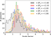 |
Fig. 1. Distributions of scale factors for the 1066 spectra of our initial sample. Each distribution represents an SDSS filter. |
We note that this rescaling does not affect other intensive quantities (scale independent), such as the stellar age and metallicity. Even by scaling the spectrum, the stellar populations that we infer from the spectrum are still representative of the area covered by the fiber, which might not be representative of the whole galaxy if radial gradients are present.
As noted above, from here on we apply the following steps described in the remainder of Sect. 3 to both the observed spectra (Case A) and the rescaled spectra (Case B) independently.
3.2. Preprocessing: Correct Milky Way extinction and rest frame
All spectra (observed and rescaled) were then converted from vacuum to air wavelengths and corrected for the Milky Way dust extinction using the dust maps of Schlafly & Finkbeiner (2011) retrieved from the NASA/IPAC Infrared Science Archive (IRSA), applying the standard Galactic reddening law with RV = 3.1 (Cardelli et al. 1989; O’Donnell 1994). After that, they were also shifted to rest-frame wavelengths.
3.3. Stellar population parameters
Galaxy spectra can be divided into two components: the stellar continuum and the ionized gas emission lines. Adopting the assumption that the star-formation history of a galaxy can be approximated as the sum of discrete star-formation bursts, the observed stellar spectrum of a galaxy can be represented as the sum of the spectra of a single stellar population (SSP) with different ages and metallicities. To infer them, we used the STARLIGHT code (Cid Fernandes et al. 2009, 2005; Mateus et al. 2006; Asari et al. 2007). STARLIGHT determines the fractional contribution of the different SSP models to the light, xi, and to the galaxy mass, μi. We can then estimate the mean light-weighted (L) or mass-weighted (M) age and metallicity of the stellar population from
 (2)
(2)
 (3)
(3)
where ti and Zi are the age and the metallicity of the ith SSP model, and wi = xi or wi = μi for light- and mass-weighted quantities, respectively. Dust effects, parametrized by  , are modeled as a foreground screen with a Cardelli et al. (1989) reddening law, assuming RV = 3.1.
We used the Granada-MILES (GM) models base of SSP models presented in Cid Fernandes et al. (2013). This base is a combination of SSP spectra from Vazdekis et al. (2010) based on stars from the Medium-resolution Isaac Newton Telescope library of empirical spectra (MILES; Sánchez-Blázquez et al. 2006) library, which start at an age of 63 Myr, with the models of González Delgado et al. (2005), which rely on the synthetic stellar spectra from the Granada library for younger ages (Martins et al. 2005). They are based on the Salpeter (1955) initial mass function (IMF) and the evolutionary tracks of Girardi et al. (2000), except for the youngest ages (< 3 Myr), which are based on Geneva tracks (Schaller et al. 1992; Schaerer et al. 1993a,b; Charbonnel et al. 1993). We selected a set of 248 SSP models with 62 different ages (from 1 Myr to 14 Gyr) for each of the four metallicities (0.2, 0.4, 1.0, and 1.5 solar).
Cid Fernandes et al. (2013) compared the stellar parameters obtained using different SSP bases, and the overall conclusion is that, from a statistical perspective, STARLIGHT results do not depend strongly on the choice of SSP models. Mean ages and extinctions all agree to within relatively small margins, and the same is true for stellar masses (once built-in differences in IMFs are accounted for).
Some wavelength regions containing known optical nebular emission lines, telluric absorptions, or strong night-sky emission lines were masked out from the fit. As an example, Fig. 2 shows the observed central spectrum of the host galaxy of SN 2005ku and the STARLIGHT fit. The fit subtraction gives the pure emission line spectrum that is used to measure the ionized gas emission lines.
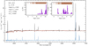 |
Fig. 2. Spectrum of the SN2005ku (SDSS10805) host galaxy (black), together with the best STARLIGHT fit (red) and the pure nebular emission line spectrum (the difference is in blue). We note that this method accounts for the absorption produced at Balmer emission line positions. In-box panels contain the distributions of the percentual contribution of the SSP models used in the STARLIGHT fit, weighted to the mass (left) and the light (right) of the host galaxy. |
In this work we focus on studying those parameters for which we have aperture corrections, so we have only made use of the stellar mass (M*) from the STARLIGHT output. Mass uncertainties were determined from repeating the fitting on 1000 realizations of the integrated spectrum, sampled from its flux and error, by adopting the width of the distribution of these 1000 values. We note that for the spectra scaled to the photometry, only extensive (scale-dependent) quantities change from the values found from the fits to the observed spectra. Intensive quantities are equivalent (see Appendix B for a comparison of the stellar parameters of Cases A and B).
3.4. Ionized gas parameters
Subtracting the STARLIGHT fits from the observed spectra, we obtain the pure nebular emission line spectra and accurately measure the flux of the most prominent emission lines (Hβ, [O III] λ5007, Hα, [N II] λ6583) by fitting a weighted nonlinear least-squares fit with a single Gaussian plus a linear term. The uncertainty of the flux was determined from the S/N of the measured line flux and the ratio between the fitted amplitude of the Gaussian to the standard deviation of the adjacent continuum. Monte Carlo simulations were performed to obtain realistic errors to the line fluxes from these two measurements. The full details of the procedure are given in Appendix C of Stanishev et al. (2012).
We needed to apply some quality cuts to our measurements. From the initial 1066 spectra, we only kept those where we simultaneously measured a S/N > 2 for all four emission lines listed above (used in the oxygen abundance estimation). In addition, we also kept galaxies whose spectra had an Hα and Hβ with a S/N > 2 independently of the S/N of the other two emission lines (used in the  and SFR measurements). In this way, we did not miss galaxies with strong Hα that can be reliably corrected for extinction using the Balmer decrement. We note that a galaxy with strong Hα and faint [N II]λ6583 is not suspected of being ionized by active galactic nucleus (AGN) emission (very low [N II]/Hα; see Sect. 3.4.1). These combined criteria allow us to be confident that we have not missed any bright Hα line used to measure the SFR or any objects with reliable oxygen abundance. We visually confirmed that these cuts leave out spectra where lines are not reliably detected. There are 869 spectra that passed the above cuts. For these objects, the HαEW was measured from the normalized spectra, resulting from the division of the actual spectra by the STARLIGHT fit. While the Hα flux is an indicator of the ongoing SFR traced by ionizing OB stars, the HαEW measures how strong this is compared to the stellar continuum, which is dominated by old low-mass non-ionizing stars and therefore accounts for most of the galaxy stellar mass. The HαEW can be thought of as an indicator of the strength of the ongoing SFR compared with the past SFR, which decreases with time if no new stars are created, and it is thus a reliable proxy for the age of the youngest stellar components (López-Sánchez & Esteban 2009; Kuncarayakti et al. 2016).
The observed ratio of Hα and Hβ emission lines provides an estimate of the gas-phase dust attenuation,  , along the line of sight through a galaxy. Assuming an intrinsic ratio I(Hα)/I(Hβ) = 2.86, valid for Case B recombination with T = 10 000 K and electron density 102 cm−3 (Osterbrock & Ferland 2006), and using the Cardelli et al. (1989) extinction law with the updated O’Donnell (1994) coefficients, we can estimate E(B − V). With this, and adopting the Milky Way average value of RV =
  /E(B − V) = 3.1, we calculated
  . The emission lines previously measured were corrected for the dust extinction before calculating any further measurement.
3.4.1. Removing AGN contribution
Some methods used to derive relevant quantities can only be applied if the ionization source exclusively arises from the stellar radiation. To identify AGN contamination in the galaxy centers, we used the Baldwin-Phillips-Terlevich (BPT; Baldwin et al. 1981; Veilleux & Osterbrock 1987) diagnostic diagram, which uses the ![Mathematical equation: $ \mathrm{O3}\equiv\log_{10}\left(\frac{{{[{\mathrm{O}\,{\textsc{iii}}}] \lambda 5007}}}{{\mathrm{H} \beta}}\right) $](/articles/aa/full_html/2022/03/aa41568-21/aa41568-21-eq9.gif) and
and ![Mathematical equation: $ \mathrm{N2}\equiv\log_{10}\left(\frac{{[{\mathrm{N}\,{\textsc{ii}}}] \lambda 6583}}{{\mathrm{H}\alpha}}\right) $](/articles/aa/full_html/2022/03/aa41568-21/aa41568-21-eq10.gif) emission line ratios and on which gas ionized by different sources occupies different areas. Two criteria commonly used to separate SF from AGN-dominated galaxies are the expressions in Kewley et al. (2001) and Kauffmann et al. (2003). However, it should be noted that the latter is an empirical expression, and bona fide H II regions can be found in the composite area determined by it (Sánchez et al. 2014). Galaxies with emission line ratios falling in the AGN-dominated region according to the criterion of Kewley et al. (2001) were excluded from the following analysis. This reduced the sample by 137 objects to 732 galaxies (see Fig. 3).
emission line ratios and on which gas ionized by different sources occupies different areas. Two criteria commonly used to separate SF from AGN-dominated galaxies are the expressions in Kewley et al. (2001) and Kauffmann et al. (2003). However, it should be noted that the latter is an empirical expression, and bona fide H II regions can be found in the composite area determined by it (Sánchez et al. 2014). Galaxies with emission line ratios falling in the AGN-dominated region according to the criterion of Kewley et al. (2001) were excluded from the following analysis. This reduced the sample by 137 objects to 732 galaxies (see Fig. 3).
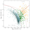 |
Fig. 3. [O III]/Hβ vs. [N II]/Hα BPT diagram of the 869 galaxies with reliable emission lines. We excluded all 137 galaxies (in orange) that fall in the region above the line by Kewley et al. (2001), which determines that the underlying ionization source is not star formation but rather an AGN. |
3.4.2. Star-formation rate
We estimated the ongoing SFR from the extinction-corrected Hα flux F(Hα) using the expression given by Kennicutt (1998):
![Mathematical equation: $$ \begin{aligned} \mathrm{SFR} \,[M_{\odot }\,\mathrm{yr} ^{-1}]=7.9365\times 10^{-42}\,L(\mathrm{H} \alpha ), \end{aligned} $$](/articles/aa/full_html/2022/03/aa41568-21/aa41568-21-eq11.gif) (4)
(4)
where L(Hα) is the Hα luminosity in units of erg s−1. Catalán-Torrecilla et al. (2015) demonstrated that the Hα luminosity alone can be used as a tracer of the current SFR, even without including UV and IR measurements, once the underlying stellar absorption and the dust attenuation effects have been accounted for, as we did here. This measurement is also used to estimate the specific SFR (sSFR; i.e., SFR/mass).
3.4.3. Oxygen abundance
Since oxygen is the most abundant metal in the gas phase and exhibits very strong nebular lines in optical wavelengths, it is usually chosen as a metallicity indicator in interstellar medium (ISM) studies.
The most accurate method to measure ISM abundances (the so-called direct method) involves determining the ionized gas electron temperature, Te, which is usually estimated from the flux ratios of auroral to nebular emission lines, for example, [O III] λ4363/[O III] λ4959 (Izotov et al. 2006; Stasińska 2006). However, the temperature-sensitive lines such as [O III] λ4363 are very weak and difficult to measure, especially in metal-rich environments that correspond to lower temperatures. Since in our data the direct method cannot be used everywhere reliably (only 16 detections with S/N > 5), we used instead other strong emission line methods to determine the gas oxygen abundance.
Many such methods have been developed throughout the years. The theoretical methods are calibrated by matching the observed line fluxes with those predicted by theoretical photoionization models. The empirical methods, on the other hand, are calibrated against H II regions and galaxies whose metallicities have been previously determined by the direct method. Unfortunately, there are large systematic differences between methods, which translate into a considerable uncertainty in the absolute metallicity scale (see López-Sánchez & Esteban 2010; López-Sánchez et al. 2012 for a review), while relative metallicities generally agree. The cause of these discrepancies is still not well understood, although the empirical methods may underestimate the metallicity by a few tenths of dex, while the theoretical methods overestimate it (Peimbert et al. 2007; Moustakas et al. 2010; Pérez-Montero 2014).
We used the O3N2 empirical method to compute the elemental abundances in all galaxies. It was first introduced by Alloin et al. (1979) as the difference between the two line ratios used in the BPT diagram ([O III]/Hβ and [N II]/Hα). Here we take the calibration introduced by Pettini & Pagel 2004,
 (5)
(5)
This method has the advantage (over other methods) of being insensitive to extinction due to the small separation in wavelength of the emission lines used for the ratio diagnostics, thus minimizing differential atmospheric refraction. It has been found to be valid for O3N2 < 2 (12 + log10O/H > 8.09). The uncertainties in the measured metallicities were computed by including the statistical uncertainties of the line flux measurements and those in the derived galaxy reddening, and by propagating them into the metallicity determination.
In summary, for all 732 remaining galaxies, we derived the  , HαEW, SFR, sSFR, and O/H.
3.5. Aperture corrections
Galaxy spectra taken with fiber or slit spectroscopy are not always comparable because different fractions are sampled, and the fraction depends on the size and distance (redshift) of each galaxy. This aperture effect is most noticeable in the low-redshift Universe, affecting the measurements of some galaxy properties, especially extensive properties (e.g., SFR) that can only increase as more light is integrated. On the other hand, the variation expected for intensive properties (e.g., O/H, and  ) is smaller.
One would be able to correct for the missing light by studying a sample of galaxies for which different fractions can be extracted and the desired parameters measured. Then, one can study how these parameters change as the integrated extent of the galaxy varies. Integral field spectroscopy is the perfect technique for approaching these problems since one can obtain multiple spectra that map the whole extent of a galaxy and simulate several spectral extractions. Iglesias-Páramo et al. (2013) estimated empirical aperture corrections from nearby galaxies observed by the CALIFA Survey (Sánchez et al. 2012). Spectra of increasing apertures were extracted from a representative sample of 165 CALIFA galaxies, and the growth of Hα, HαEW, and the ratio of Hα/Hβ were studied for different galaxy morphologies, inclinations, and masses. Further analysis, with a larger sample, of the growth of the ratio of [N II]/Hα and [O III]/Hβ, the line ratios used for the estimation of the oxygen abundance with the O3N2 calibrator, was also presented in Iglesias-Páramo et al. (2016) and Duarte Puertas et al. (2017). These works provided growth curves for all these measurements normalized to the total integrated value at 2.5 R50, where R50 is the Petrosian radius containing 50% of the total galaxy flux in a particular band. The growth curves used in this work described as fifth-order polynomials are summarized in Table 1.
Results of the fifth-order polynomial fits to the fixed angular aperture corrections given in Iglesias-Páramo et al. (2013, 2016), in the form a0 + a1 * x + a2 * x2 + a3 * x3 + a4 * x4 + a5 * x5, where x is r/R50.
These aperture corrections have two caveats: (i) for large and very nearby galaxies, the fiber covers only a very small fraction, r/R50, of the galaxy, and aperture corrections would have huge errors. For this reason, Iglesias-Páramo et al. give tabulated values starting from r/R50 = 0.3; and (ii) for apparently small and/or high-redshift galaxies for which the galaxy size is comparable to the seeing of the observation, R50 is not well defined since it measures the half light of the point spread function and cannot account for the shape of the galaxy. For such small or far galaxies, no aperture correction is needed.
The final goal of applying these aperture corrections is to be able to make proper comparisons among galaxies for all parameters within a range of redshifts, as if the fiber covered the same extent in all galaxies. Here we made use of the information presented in these two studies to correct the host galaxy parameters measured in previous sections. For that, we obtained the R50 parameter in the r band from the SDSS database and calculated the area covered by either the SDSS or the BOSS fiber as a fraction of R50. Therefore, by comparing the coverage for each galaxy to the tabulated values, one can apply a simple correction factor to the values estimated in the previous sections.
Considering only those galaxies that fulfilled the condition of having a coverage of r > 0.3 R50, and with the values for the fiber radius being 1″ for BOSS and 1.5″ for SDSS, only eight galaxies were removed. As such, we kept 724 galaxies.
In Appendix C we provide the final measurements of the main properties for the three cases (A, B, and C) that are used in the following sections. These include the scaled galaxy stellar mass, the SFR, the oxygen abundance, the HαEW, and the  .
.
4. The effect of aperture corrections on derived properties
In this section we focus on the effect that aperture corrections have on the physical parameters of SN host galaxies for the three different cases of interest: (i) Case A, observed fiber spectra; (ii) Case B, observed fiber spectra scaled to the global galaxy photometry; and (iii) Case C, observed fiber spectra corrected for aperture effects.
The first row of Fig. 4 shows the SFR – M⋆ relation for Cases A, B, and C, from left to right. In each panel, we performed a linear fit only to the SF galaxies (the main sequence of this relation). In the lower panel of Case C we show the difference between both the Case A and B fits and the Case C fit. From the differences in the linear fits we found that at a fixed stellar mass the SFR values in Case C are on average higher than in Cases A and B across the stellar mass range between 108.5 and 1012.0 M⊙. Most importantly, the residuals show a trend with stellar mass, implying a mass-dependent bias in the inferred SFR without considering aperture effects: these differences are higher at low stellar masses (0.45 and 0.20 dex for A and B linear fits, respectively) than at the higher end (0.18 and 0.06 dex for A and B, respectively). Therefore, regardless of whether the Hα flux has been scaled or not, if it is not corrected for aperture effects, the SFR value is underestimated in the entire range of stellar masses between 108.5 and 1012.0 M⊙.
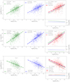 |
Fig. 4. SFR–M⋆, O/H–M⋆, and sSFR–M⋆ relations for our sample of galaxies. Star-forming (colored crosses) and composite (gray triangles) galaxies based on the BPT classification are represented in each diagram. The left and central panels correspond to Case A and Case B, respectively. We included the linear fit of the SFR–M⋆ relation for all the SF galaxies. The right panels correspond to Case C, with the aperture corrected. In the upper panel we include the linear fit of the SFR–M⋆ relation for all the SF galaxies considered in Case C (dashed red line), the fit from Case A (dotted green line), and the fit from Case B (dotted blue line). In the bottom-right panel, the sSFR–M⋆ relation, we also include a fourth relation (dotted red) that corresponds to an aperture-corrected SFR (Case C) normalized to the mass measured in the fiber spectrum (Case A). In the lower panels we show the difference between the linear fit in Case C and the linear fits of Case A (dotted green line) and Case B (dotted blue line). |
In the central row of the same figure, Fig. 4, we repeated the same analysis, this time for the O/H – M⋆ relation. From the differences in the linear fits shown in the lower panel, we found that the aperture-corrected values of O/H at a fixed stellar mass are slightly lower than the values obtained in Cases A and B for the stellar mass range between 108.5 and 1012.0 M⊙. These differences are small in the whole stellar mass range considered (lower than 0.1 dex), as expected for intrinsic parameters.
In the bottom row of Fig. 4 we show the sSFR – M⋆ relation in each case. In addition, for Case C we show the linear fit of the sSFR values in the fiber (we note that it is not the same value as in Case A since the stellar masses considered for Case C are scaled). Considering these differences in the fits, we found that on average at a fixed stellar mass the sSFR values in Case C are higher than in Cases A and B across the entire stellar mass range between 108.5 and 1012.0 M⊙. Differences are higher at low stellar masses (0.45 and 0.30 dex for A and B, respectively) than at high stellar masses (0.18 and 0.06 dex for A and B, respectively). When we compared the sSFR in Case C (using only the scaled stellar mass) for Hα flux both corrected and uncorrected for aperture, we found that the difference between them increases with the stellar mass (from 0.30 dex at 108.5 M⊙ to 0.54 dex at 1012.0 M⊙).
In Fig. 5 we show the histogram of the differences between Cases C and A (aperture-corrected vs. observed) as well as between Cases C and B (aperture-corrected vs. scaled) for the SFR, O/H, and sSFR. In addition, we also show the difference in  between Case C and Case A. When aperture corrections are not taken into account, the SFR value is underestimated by ∼0.44 dex on average when comparing Cases C and A, and ∼0.13 dex when comparing Cases C and B. The average difference of Δ(12+log(O/H)) is ≃0.025 dex in both cases (C-A and C-B), so aperture-corrected abundances are almost always lower. When we considered the differences in the sSFR values between Cases C and A and between Cases C and B, we obtain a difference of ∼0.13 dex in both cases. Taking into account the galaxies of Case C, when we compared the sSFR values with the SFR measurement corrected and uncorrected for aperture effects, we recovered the average difference of ∼0.44 dex found in the upper-left panel. Finally, we found that the median of the difference between the aperture-corrected and the uncorrected
  (
( ) is −0.16 mag.
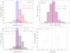 |
Fig. 5. Distribution of the differences of the studied parameters among cases. Upper-left panel: histogram of the differences in SFR values for Cases C and A (red) and Cases C and B (blue). Upper-right panel: histogram of the differences in 12+log(O/H) values for Cases C and A (red) and Cases C and B (blue). Lower-left panel: histogram of the differences in sSFR values for Cases C and A (red), Cases C and B (blue), and with the SFR corrected but divided by the observed mass within the fiber (gray). Lower-right panel: histogram of the differences in |

4.1. Comparison to fiber fraction galaxy coverage
Kewley et al. (2005) found that for an emission line metallicity measurement to be representative of the global value, the spectrum should contain > 20% of the host galaxy g-band flux. Kewley & Ellison (2008) claimed that this g-band flux fraction had to be > 30% for galaxies with M > 1010 M⊙. In either case, this translates to excluding from any metallicity analysis all galaxies with a relatively less concentrated g-band flux or galaxies larger in size.
Thus, the fraction of the total host galaxy light covered by the fiber is an important quantity to consider in this analysis. Fortunately, spectra obtained as a part of the SDSS survey have fiber and model magnitudes associated with each galaxy, so we can easily compute the observed light fraction in the spectra and compare the resulting sample with that derived in our approach, which only depends on the Petrosian R50 parameter.
In the left panel of Fig. 6, we examine the g-band fiber fraction for the initial 732 galaxies before applying our aperture corrections, as a function of the total g band of galaxies. We see a clear relation between these two parameters in the direction of fainter galaxies, which in turn are also smaller, having a larger area covered by the fiber. The criteria of selecting galaxies with g-band fiber coverage larger than 20% would have excluded 159 galaxies, shown under the gray region in this panel. In the central panel we compare the two criteria, the g-band light fraction and the fiber radius in R50 units. Despite the tight relation between the two parameters, the different criteria for discarding galaxies provide samples of significantly different sizes: from the initial 732 galaxies, we kept 573 and 724, respectively. Finally, in the right panel we show the redshift dependence of the fiber radius in R50 units. It can clearly be seen that the eight galaxies in the exclusion zone are both at the lower-redshift end and with very low fiber radii in R50 units, and are thus large in size. We also marked with black edges those galaxies that pass our criterion for aperture corrections but where the fiber did not cover 20% of the g-band light and thus would have been excluded following the other criterion.
 |
Fig. 6. Comparison between the remaining sample of galaxies once the g-band fraction or aperture correction criteria are considered. Left:g-band flux fraction covered within the fiber with respect to the total magnitude (“modelMag” in the SDSS catalogue) of the galaxy. The horizontal line at 0.2 corresponds to the cut suggested by Kewley et al. (2005) and used in D’Andrea et al. (2011) and Wolf et al. (2016) to justify that objects below the line on the shaded region have spectra that are not representative of the whole galaxy and therefore were excluded from those analyses. Middle:g-band fiber flux fraction vs. radii of the galaxy normalized to the Petrosian R50 radius (radius of a circle that contains 50% of the galaxy light). The horizontal line is the Kewley et al. (2005) limit, under which all objects (in the shaded region) would be excluded. The vertical line corresponds to the range where our aperture corrections are applied, and objects in the shaded region to the left (r/R50 < 0.3) are excluded because Iglesias-Páramo et al. (2013, 2016) corrections cannot be applied. We note that those galaxies with r/R50 ≥ 0.3 (to the right of the vertical line) but a g-band fiber flux fraction lower than 0.2 (below the horizontal line) would have been excluded but are included in this work. Right: normalized radii (r/R50) of the galaxies vs. redshift. Dots with black edges correspond to the 159 objects that we would have discarded using the g-band fraction criterion. In our selection we have mostly lost galaxies at low redshifts. |
So, we have shown here that under our approach we are able to both (a) correct the measured host galaxy parameters for aperture effects and (b) keep a larger number of objects for the study of SN host galaxy correlations.
4.2. Biases on host galaxy parameters
Here we also show that our sample selection based on the availability of aperture corrections not only maximizes the number of objects for the analysis, but also avoids the introduction of biases in the host galaxy distributions.
Previous works similar to ours have followed the g-band fraction criterion (e.g., D’Andrea et al. 2011). For instance, one of the most recent, Wolf et al. (2016), found little correlation between the g-band fiber fraction and gas-phase metallicity, indicating that aperture corrections were not needed.
In Fig. 7 we present the relation between the g-band fiber galaxy fraction and the fiber coverage in R50 units with the stellar mass, oxygen abundance, sSFR, and HαEW. While it is evident that the few objects that are excluded using the R50 criterion for aperture corrections correspond to outliers, we demonstrate how the g-band fraction selection tends to remove from the sample large mass, high-metallicity, low-sSFR, and low-HαEW galaxies.
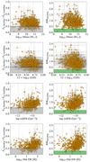 |
Fig. 7. g-band fraction (left column) and galaxy radius covered by the fiber in R50 units (right column) as a function of the main galaxy parameters used in this work: stellar mass, oxygen abundance, sSFR, and HαEW. The shadowed regions represent the regions excluded under each criterion. This figure clearly shows that under one criterion fewer objects are excluded, and it shows the tendency to exclude objects with higher or lower values for each galaxy parameter. |
Summarizing, the approach followed in this work permits the use of a significantly larger fraction of objects relative to other approaches, corrects for aperture effects, and avoids selection biases in host galaxy distributions.
5. SN light-curve parameters
To study the intrinsic relationship between the properties of a SN Ia and its host, we used the light-curve parameters as published in the SDSS-II SNS DR (Sako et al. 2018), which were obtained using the SALT2 template implemented in the publicly available Supernova Analyzer (SNANA) package (Kessler et al. 2009b).
In the SALT2 model, four parameters – namely the epoch of maximum brightness in the B band (t0), the color of the SN (c) at peak, the x1 parameter (related to the stretch of the light curve), and the x0 normalization factor (from which one can obtain the apparent magnitude at maximum brightness in the B band; mB) – are determined from the fit to the multiband light curve. Standardized magnitudes are obtained using the Tripp equation,
 (6)
(6)
where M, α, and β are nuisance parameters that result from minimizing the difference between μSALT2 and the distance modulus assuming a fiducial cosmology. Since our goal is not to measure the best cosmology from our data but to look for systematic effects with aperture-corrected host galaxy parameters and correlate the residuals from the distances measured with SNe Ia to that cosmology, in our case we used the μSALT2 values reported in Sako et al. (2018) for the nuisance parameters (M, α, β) = (−29.967, 0.187 ± 0.009, 2.89 ± 0.09) and calculated Hubble residuals by subtracting the distance modulus of a flat cosmology from them (HR = μSALT2 − μcosmo). To assure a robust sample of SNe Ia unaffected by peculiar objects, we discarded SNe Ia with a SALT2 probability of being a SN Ia (SNANA parameter FITPROB) < 1%. In addition, we removed all SNe with extreme light-curve parameter values following standard selection cuts for SALT2, so the allowed ranges are set to −0.3 < c < 0.3, −3.0 < x1 < 3.0, and −1.0 < HR< 1.0 (Sako et al. 2018). These cuts were designed to remove objects with peculiar or badly constrained light curves. From our list of 724 and 573 SNe Ia with measured host galaxy parameters in the aperture-corrected and the g-band fraction samples, we are left with a final sample of 589 and 475 SNe Ia, respectively.
Figure 8 shows the distribution of SALT2 c and x1 parameters and the Hubble residuals for all the SNe Ia in the SDSS-II SNS DR and similar distributions for our final sample. All distributions have equivalent shapes and statistics (⟨x1⟩ = 0.11, σx1 = 1.12; ⟨c⟩= − 0.01, σc = 0.11; ⟨HR⟩ = 0.00, σHR = 0.27), but it is evident how the sample decreased in size from the initial to the aperture-corrected sample, and even more to the g-fraction sample.
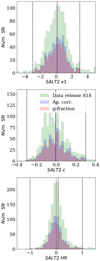 |
Fig. 8. x1 and c light-curve parameter and Hubble residual distributions of the full SDSS-II DR (green) compared to those of the samples after applying the fiber radius in R50 units (blue) and the g-band fraction (in red) cuts used here. Vertical colored lines represent the mean of the samples, and dashed black lines define the quality selection range. |
6. Results and discussion
We present SN Ia light-curve parameters and Hubble residual correlations with host galaxy parameters in Fig. 9, separately for the 589 objects in the aperture-corrected sample (our fiducial sample, as blue dots) and the 475 objects in the g-fraction sample (the literature approach sample, in red circles). We performed two kinds of analyses: (i) “step” functions: we divided the sample into two bins of the same size using the independent variable in the X axis to then measure the mean, mean error, and standard deviation of the dependant variable in the Y axis in each of the two bins; (ii) we performed a linear fit with LINMIX1 (Kelly 2007), which is more robust than a simple least-squares linear fit because it takes into account the errors in both X-axis and Y-axis variables, and also because it computes a probability function for the data set using a Markov chain Monte Carlo (MCMC) algorithm. A summary of all slopes and steps are listed in Table 2. Overplotted in each panel of Fig. 9, we show the best fit from LINMIX (thick solid line) plus the 10 000 minimizations with transparency.
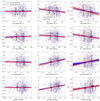 |
Fig. 9. x1, c, and Hubble residual correlations with host galaxy parameters – stellar mass, oxygen abundance, sSFR, and HαEW – for the aperture-corrected sample (in blue) and the g-band fraction sample (in red). Solid transparent lines are the 10 000 individual slopes found with the LINMIX MCMC sampler, with the average slope as a solid line on top. Overplotted there are the average and standard deviation of the variable on the Y-axis in each of the two high and low bins in the X-axis variable, which has been divided using the median X value as the split point. The height of the box represents the error of the mean in each bin. |
Results of the LINMIX MCMC slopes and the difference (steps) between the high and low bin.
6.1. Recovering mass step
We started testing whether the Hubble residuals of our resulting samples conserve a dependence with the host galaxy mass as reported by several works, including those using SDSS-II SNS data. As noted above, the host mass is not a parameter for which we have aperture corrections available, and therefore we focus on how different the dependence is in the two final samples due to possible bias introduced by the selection criterion.
In the first row of Fig. 9 we show the light-curve parameters c and x1 together with the Hubble residuals as a function of the scaled mass (Case B) for the SNe Ia in the aperture-corrected (blue) and g-fraction (red) samples. While we find a low significance (< 1.3σ) mass step in the color parameter, we find a 2–4σ step in the x1 and Hubble residuals. The mass step is higher and more significant in the g-band fraction sample than in the aperture-corrected sample, which in principle contains a wider and more complete set of host galaxy parameters. In particular, we showed in Sect. 4.2 that removing objects with a small g-band fraction tends to get rid of higher-mass galaxies. It is evident in the upper-right panel of Fig. 9, which shows Hubble residuals versus mass, that most of the blue points at larger masses are not included in the g-band sample, and most of them have positive Hubble residuals. Therefore, the g-band fraction criterion introduces a selection bias since it preferentially tends to include galaxies whose light is more concentrated (elliptical morphology, early-type). Since these galaxies on average host SNe with particular properties, the net effect is to artificially increase the height of the mass step.
In Fig. 10 we demonstrate these two (and other) biases with distributions of the SN Ia light-curve parameters, Hubble residuals, and host galaxy parameters for the 114 objects that are present in the aperture-corrected sample but that did not pass the g-band fraction criterion. These objects have slightly larger x1 (∼0.15), c (∼0.02), and Hubble residuals (∼0.04 mag) than the average value in the aperture-corrected sample. Moreover, they show an average stellar mass that is ∼0.34 dex larger then the average mass of the aperture-corrected sample. The net effect of the g-band fraction criterion is that intrinsically faint SNe Ia in higher-mass galaxies are discarded, thus artificially increasing the height of the mass step.
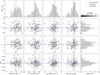 |
Fig. 10. SN Ia light-curve x1 and c parameters and Hubble residual dependences on stellar mass, oxygen abundance, sSFR, and HαEW of the 114 objects that are discarded using the g-band fraction criterion. Black lines represent the mean of the distribution, and red and blue lines represent the mean of the g-band fraction and aperture-corrected samples, respectively. Regarding light-curve parameters and Hubble residuals, while the three original distributions are centered at zero, these discarded objects have positive averages in the three distributions, leaving on average more negative biased distributions in the g-band fraction sample. Moreover, discarded objects have, on average, a larger stellar mass, lower HαEW, lower sSFR, and higher metallicity with respect the aperture-corrected sample, so the g-band fraction criterion also leaves a sample of SNe Ia and host galaxies that are biased toward the other side of the distributions. |
6.2. SN light-curve dependences on corrected host galaxy parameters
In the bottom three rows of Fig. 9 we present the dependence of light-curve parameters and Hubble residuals with the host galaxy oxygen abundance, sSFR, and HαEW. Our assumption throughout this work is that the aperture-corrected sample is unbiased with respect to the selection performed by removing all galaxies with fiber fractions smaller than a certain limit. The relations found in the aperture-corrected sample are therefore the true underlying correlations of x1, c, and the Hubble residuals, with the late-type SF host galaxy environmental parameters.
We find a significant trend between the x1 parameter and the Hubble residual and both the sSFR and HαEW (3–6σ), in the sense of wider and intrinsically faint (positive Hubble residual) SNe Ia occurring in galaxies with higher sSFRs and HαEWs, consistent with previous findings (e.g., Sullivan et al. 2006, 2010). On the other hand, the c steps are on the order of 1σ, while the slope is insignificant. Specific SFR is measured by dividing the aperture-corrected Hα flux (Case C) by the scaled stellar mass (Case B). It therefore represents the efficiency of a galaxy to form stars normalized by the total mass of the stars present. On the other hand, HαEW is the ratio of the Hα flux over the flux of the continuum, so it provides a measurement of the intensity of the current star formation compared to the past SFR. Although similar, the information these two indicators provide is not exactly the same. Although these correlations are present in both samples, in general (in all cases except in the step of the sSFR), they are marginally increased in the g-band fraction sample. Thus, the sample selection also introduces a bias in the sample toward increasing the significance of these correlations.
Regarding oxygen abundance, we find insignificant relations with the c parameter (< 1σ), in the sense of bluer SNe Ia occurring in higher-metallicity galaxies, which is marginally increased in the aperture-corrected sample. Lower significance (2–3σ) trends are found with x1 and Hubble residuals, where negative x1 and negative Hubble residuals tend to occur in high-metallicity galaxies. In particular, we find a metallicity step in the Hubble residual with a significance of ≳2σ. All these are in line with previous results in the literature (D’Andrea et al. 2011; Moreno-Raya et al. 2018). Similarly, the g-band fraction results have higher significance with Hubble residuals, pointing to a selection bias.
Again, in Fig. 10 the distribution of these other host galaxy parameters are shown for the 114 SNe Ia in the sample discarded using the g-band fraction criterion, together with the correlations between them and the light-curve parameters and Hubble residuals. Discarded objects have on average an oxygen abundance 0.04 dex higher, a log10sSFR = −0.25 dex lower, and log10HαEW = −0.12 dex lower than both the full aperture-corrected and the g-band fraction selected samples. These differences explain the varying significance between the two main samples in all relations. Moreover, we note that for the aperture-corrected sample the step significance with environmental parameters is sorted from higher to lower as (see Table 2)
 (7)
(7)
while for the g-fraction sample it is
 (8)
(8)
Besides the difference in the sorted parameters, we note how in the fiducial sample both the sSFR and the HαEW show a greater significance than the galaxy stellar mass. As detailed above, although the sSFR and HαEW do not exactly provide the same information about the underlying stellar populations, they are both proxies for the stellar population age. Therefore, our findings indicate that, once the selection biases are removed, the stellar population age seems to have a greater impact on the standardization of SNe Ia than the stellar mass (as pointed out by Rose et al. 2019). Historically, mass has been widely used in cosmological analyses to improve the standardization, and the mass step is now a common term added to the Tripp equation (Betoule et al. 2014; Brout et al. 2019). This is partially explained by the simplicity of its measurement; several works have found that with just a few photometric points mass can be constrained with high accuracy (Childress et al. 2013a; Hand et al. 2022). Stellar age is more difficult to constrain, especially with photometric data alone. It is notably degenerate with stellar metallicity and dust reddening, and it is better determined from spectroscopy or with complementary UV and NIR data.
Similarly to Roman et al. (2018), we studied whether the information encapsulated in the sSFR can be recovered with the stellar mass alone by performing the following test: for each of the four host galaxy parameters in Fig. 9, we corrected the higher bin of the Hubble residual relation by the height of the measured step and looked again for the correlations. While after correcting for the mass step we still find a > 2σ significance in the sSFR and HαEW steps, the significance of the mass step is < 2σ once either the sSFR or the HαEW step is corrected for. This may indicate that the sSFR and HαEW, the parameters more related to the age of the underlying stellar populations, do a better job in improving SN Ia standardization than stellar mass. In the case of metallicity, when its step is corrected, the significance of the other three steps is reduced by 0.5–0.7σ and they remain significant at the 3σ level. Also interesting is that when any of the other three steps are corrected for, the remaining metallicity step is insignificant (< 0.2σ), indicating that the information captured by the metallicity is already included in either the mass or the stellar age.
6.3. Cosmological parameter determination
Table 2 shows the relations between the Hubble diagram residuals and galaxy properties we found for both the aperture-corrected sample and g-band fraction sample. With each subsample being prone to different selection effects, we test here the effect that these relationships have on the derived cosmological parameters.
To determine the cosmological parameters, we replicated the selection criteria of Sako et al. (2018): restricting our analysis to spectroscopically confirmed events, enforcing −2 < x1 < 2 and −0.2 < c < 0.5, and removing objects with poorly measured x1 (i.e., σx1 < 2). These selection criteria reduce the aperture-corrected sample to 190 SNe Ia, compared to 122 for the g-band fraction sample and 413 for the SDSS sample. To estimate the distance to each SN, we used the best-fit nuisance parameters determined in Sako et al. (2018), namely α = 0.155, β = 3.17, and M0 = −29.967, and applied the Tripp formula (Tripp 1998). Based on these distances, we then constrained the cosmological parameters: in particular, the matter and dark-energy density (Ωm, ΩΛ), marginalizing over H0 using an MCMC approach.
In the upper panel of Fig. 11 we show the resulting cosmological constraints from all three samples, where the sizes of the contours clearly increase as the sample size is reduced. Going one step further, and assuming a flat ΛCDM model (i.e., Ωλ = 1 − Ωm), we recover best-fit estimates of  for the SDSS sample,
  for the aperture-corrected sample, and
  for the g-band fraction sample, as shown in the bottom panel of Fig. 11. All estimates are consistent at < 1σ, indicating that selection biases, while different for each sample, do not overly bias the cosmological parameters.
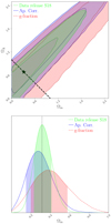 |
Fig. 11. Cosmological constraints. Top: constraints on Ωm, ΩΛ when considering the aperture-corrected sample (blue), compared to the g-band fraction sample (red) and the entire SDSS sample (green). The best-fit value for the SDSS data set, assuming a flat ΛCDM model (plotted as a dashed black line) is shown as a black star. Differences in the contours are primarily due to different host galaxy selection. Bottom: 1D, marginalized contours for Ωm are shown for the three samples, once a flat ΛCDM cosmology is assumed. |
Subtracting off the best-fit model ( ) for each sample, we find a root-mean-square (RMS) scatter of 0.183 for the SDSS sample, 0.167 for the aperture-corrected sample, and 0.174 for the g-band fraction sample. The RMS is largest for the SDSS sample, which probes the largest redshift range and hence includes the lowest signal-to-noise SNe of all three samples. Conversely, the smallest RMS is to be found in the aperture-corrected sample, which includes additional low-redshift and, hence, higher signal-to-noise events than the g-band fraction sample. This result suggests that selecting events based on fiber fraction as opposed to aperture corrections will not only cause additional bias in the sample selection, but will likely degrade the inferred cosmological parameters due to the lost of bright, low-redshift, anchor events. We also note that the relative error on Ωm is smaller for the aperture-corrected sample than for the g-band fraction sample even after taking the larger sample size and increased redshift leverage of the aperture-corrected sample into account. This result may hint that future cosmological surveys will improve their constraints on the equation-of-state of dark energy by using aperture corrections when inferring galaxy properties simply because of the reduced uncertainties due to selection effects in this approach.
6.4. Extinction parameter
We find no significant dependence between any of the light-curve parameters or Hubble residuals and the extinction parameter,  . To look further into the dependence of the extinction with host galaxy parameters, and motivated by the recent studies by Brout & Scolnic (2021) and González-Gaitán et al. (2021), we present in Fig. 12 how the measured visual extinction varies as a function of the other host galaxy parameters. As we have shown in Sect. 3.5, aperture-corrected extinction tends to be lower than extinction measured by scaling the spectrum by 0.16 mag on average.
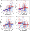 |
Fig. 12. Visual extinction as a function of the main host galaxy parameters studied in this work. Blue and red symbols represent the aperture-corrected and the g-band fraction samples, respectively. The box widths represent the error of the mean, and the vertical lines represent the scatter in that bin. |
Low-mass galaxies show lower values and with a lower spread in extinction compared to galaxies with higher masses, as previously pointed out by Garn & Best (2010). Extinction tends to mildly increase with oxygen abundance, and the dispersion is lower in metal-rich galaxies than in their metal-poorer counterparts. Regarding the sSFR and HαEW, we find different but equivalent behaviors: galaxies with low sSFRs and galaxies with large HαEWs have lower extinction values and with lower spread.
The behavior in the aperture-corrected and g-band fraction samples is quite similar, and apart from the shift in values we do not find a significant difference among samples. A more in-depth analysis using different RV parameters for each SN Ia or for populations (e.g., low and high-mass bin), and how this may affect host galaxy environmental dependences, is beyond the scope of this paper but is a topic of ongoing research.
7. Conclusions
This is the third in a series of papers where we study how the environment affects SN Ia properties; in our earlier papers we presented a SN Ia absolute magnitude dependence on the environmental metallicity (Moreno-Raya et al. 2016) and a revised study of SN Ia light-curve parameters and distance correlations with spectroscopic host galaxy parameters (Moreno-Raya et al. 2018). Here, we used the published sample of SNe Ia observed by the SDSS-II SNS to look for correlations between the SN light-curve parameters and spectroscopic host galaxy parameters from spectra available in SDSS DR16. We used the SSP synthesis technique to measure the stellar population parameters of the host galaxies and, after removing the stellar contribution, the gas emission parameters. We applied aperture corrections derived from IFS provided by the CALIFA Survey to the measured parameters and obtained values that are representative of the whole galaxy, removing the different fiber coverage of each galaxy.
Compared to other methods used in previous works, such as the fraction of the total g-band flux collected in the fiber, we demonstrate that applying these corrections avoids biasing the sample of galaxies available for the study of SN Ia light-curve and distance correlations with their environmental properties. In particular, the net effect of the g-band fraction criterion is discarding intrinsically faint SNe Ia in higher-mass galaxies, thus artificially increasing the height of the mass step. We find equivalent biases in other environmental parameters: high-metallicity, low-sSFR, and low-HαEW galaxies are similarly removed using the g-fraction criterion, leaving biased samples toward the opposite direction. The order of significance in the Hubble residual dependence between the two samples switches from the stellar mass to the sSFR being the most significant in the biased and unbiased samples, respectively.
The novel approach presented here could be performed in the future with a larger and more complete sample of SNe Ia, such as the Dark Energy Survey (DES) SN sample, which has been complemented with the fiber spectroscopy of their host galaxies by the Australian Dark Energy Survey (OzDES; Lidman et al. 2020) project. Similarly, in a few years the same method could also be applied to the Legacy Survey of Space and Time (LSST) SN Ia host galaxy spectroscopy that will be collected by dedicated fiber-spectroscopy surveys such as the Dark Energy Science Instrument (DESI; Flaugher & Bebek 2014) and the Time-Domain Extragalactic Survey (TiDES; Swann et al. 2019) within the 4-metre Multi-Object Spectroscopic Telescope (4MOST; de Jong et al. 2019) consortium.
Improvements on the corrections presented here would include a complementary IFS project that obtains observations of most or all galaxies that host SNe discovered by a SN survey. Of course, this would be expensive in terms of time and resources. One has to balance the more precise and higher quality data provided by IFS and the availability of larger samples of galaxies provided by massive fiber-spectroscopic surveys. Current samples of SN Ia host galaxies observed with IFS such as the PMAS/PPak Integral-field Supernova Hosts Compilation (PISCO; Galbany et al. 2018) and the All-weather MUse Supernova Integral-field Nearby Galaxies (AMUSING; Galbany et al. 2016a) survey are helping to fill this gap, compiling a large sample of objects to allow environmental studies of SNe Ia and their host galaxies with high quality observations.
Acknowledgments
L.G. acknowledges financial support from the Spanish Ministerio de Ciencia e Innovación (MCIN), the Agencia Estatal de Investigación (AEI) 10.13039/501100011033, and the European Social Fund (ESF) “Investing in your future” under the 2019 Ramón y Cajal program RYC2019-027683-I and the PID2020-115253GA-I00 HOSTFLOWS project, and from Centro Superior de Investigaciones Científicas (CSIC) under the PIE project 20215AT016. M.S. is funded by the European Reearch Council (ERC) under the European Union’s Horizon 2020 Research and Innovation program (grant agreement no 759194 – USNAC). S.D.P. is grateful to the Fonds de Recherche du Québec – Nature et Technologies. SGG acknowledges support by FCT under Project CRISP PTDC/FIS-AST-31546/2017 and Project No. UIDB/00099/2020. S.D.P., J.I.P., J.M.V. acknowledge support from the Spanish Ministerio de Economía y Competitividad under grant PID2019-107408GB-C44, and Junta de Andalucía Excellence Project P18-FR-2664, and from the State Agency for Research of the Spanish MCIU through the ‘Center of Excellence Severo Ochoa’ award for the Instituto de Astrofísica de Andalucía (SEV-2017-0709). Escrit en part al Bellver, prop del mugró del Tagamanent, sobre la vall de ciment malalta (J.G., center forward).
References
- Ahumada, R., Prieto, C. A., Almeida, A., et al. 2020, ApJS, 249, 3 [Google Scholar]
- Alloin, D., Collin-Souffrin, S., Joly, M., & Vigroux, L. 1979, A&A, 78, 200 [Google Scholar]
- Asari, N. V., Cid Fernandes, R., Stasińska, G., et al. 2007, MNRAS, 381, 263 [Google Scholar]
- Baldwin, J. A., Phillips, M. M., & Terlevich, R. 1981, PASP, 93, 5 [Google Scholar]
- Betoule, M., Kessler, R., Guy, J., et al. 2014, A&A, 568, A22 [NASA ADS] [CrossRef] [EDP Sciences] [Google Scholar]
- Brout, D., & Scolnic, D. 2021, ApJ, 909, 26 [NASA ADS] [CrossRef] [Google Scholar]
- Brout, D., Scolnic, D., Kessler, R., et al. 2019, ApJ, 874, 150 [NASA ADS] [CrossRef] [Google Scholar]
- Burns, C. R., Parent, E., Phillips, M. M., et al. 2018, ApJ, 869, 56 [Google Scholar]
- Campbell, H., D’Andrea, C. B., Nichol, R. C., et al. 2013, ApJ, 763, 88 [Google Scholar]
- Cardelli, J. A., Clayton, G. C., & Mathis, J. S. 1989, ApJ, 345, 245 [Google Scholar]
- Catalán-Torrecilla, C., Gil de Paz, A., Castillo-Morales, A., et al. 2015, A&A, 584, A87 [NASA ADS] [CrossRef] [EDP Sciences] [Google Scholar]
- Charbonnel, C., Meynet, G., Maeder, A., Schaller, G., & Schaerer, D. 1993, A&AS, 101, 415 [NASA ADS] [Google Scholar]
- Childress, M., Aldering, G., Antilogus, P., et al. 2013a, ApJ, 770, 108 [Google Scholar]
- Childress, M., Aldering, G., Antilogus, P., et al. 2013b, ApJ, 770, 107 [NASA ADS] [CrossRef] [Google Scholar]
- Cid Fernandes, R., Mateus, A., Sodré, L., Stasińska, G., & Gomes, J. M. 2005, MNRAS, 358, 363 [Google Scholar]
- Cid Fernandes, R., Schoenell, W., Gomes, J. M., et al. 2009, Rev. Mex. Astron. Astrofis. Conf. Ser., 35, 127 [Google Scholar]
- Cid Fernandes, R., Pérez, E., García Benito, R., et al. 2013, A&A, 557, A86 [NASA ADS] [CrossRef] [EDP Sciences] [Google Scholar]
- D’Andrea, C. B., Gupta, R. R., Sako, M., et al. 2011, ApJ, 743, 172 [Google Scholar]
- de Jong, R. S., Agertz, O., Berbel, A. A., et al. 2019, Messenger, 175, 3 [Google Scholar]
- Dhawan, S., Jha, S. W., & Leibundgut, B. 2018, A&A, 609, A72 [NASA ADS] [CrossRef] [EDP Sciences] [Google Scholar]
- Dilday, B., Kessler, R., Frieman, J. A., et al. 2008, ApJ, 682, 262 [Google Scholar]
- Dilday, B., Smith, M., Bassett, B., et al. 2010, ApJ, 713, 1026 [NASA ADS] [CrossRef] [Google Scholar]
- Duarte Puertas, S., Vilchez, J. M., Iglesias-Páramo, J., et al. 2017, A&A, 599, A71 [NASA ADS] [CrossRef] [EDP Sciences] [Google Scholar]
- Flaugher, B., & Bebek, C. 2014, in Ground-based and Airborne Instrumentation for Astronomy V, eds. S. K. Ramsay, I. S. McLean, & H. Takami, SPIE Conf. Ser., 9147, 91470S [NASA ADS] [Google Scholar]
- Frieman, J. A., Bassett, B., Becker, A., et al. 2008, AJ, 135, 338 [Google Scholar]
- Fukugita, M., Ichikawa, T., Gunn, J. E., et al. 1996, AJ, 111, 1748 [Google Scholar]
- Galbany, L., Miquel, R., Östman, L., et al. 2012, ApJ, 755, 125 [NASA ADS] [CrossRef] [Google Scholar]
- Galbany, L., Stanishev, V., Mourão, A. M., et al. 2014, A&A, 572, A38 [NASA ADS] [CrossRef] [EDP Sciences] [Google Scholar]
- Galbany, L., Anderson, J. P., Rosales-Ortega, F. F., et al. 2016a, MNRAS, 455, 4087 [NASA ADS] [CrossRef] [Google Scholar]
- Galbany, L., Stanishev, V., Mourão, A. M., et al. 2016b, A&A, 591, A48 [NASA ADS] [CrossRef] [EDP Sciences] [Google Scholar]
- Galbany, L., Anderson, J. P., Sánchez, S. F., et al. 2018, ApJ, 855, 107 [Google Scholar]
- Gallagher, J. S., Garnavich, P. M., Berlind, P., et al. 2005, ApJ, 634, 210 [NASA ADS] [CrossRef] [Google Scholar]
- Garn, T., & Best, P. N. 2010, MNRAS, 409, 421 [Google Scholar]
- Girardi, L., Bressan, A., Bertelli, G., & Chiosi, C. 2000, A&AS, 141, 371 [NASA ADS] [CrossRef] [EDP Sciences] [Google Scholar]
- González Delgado, R. M., Cerviño, M., Martins, L. P., Leitherer, C., & Hauschildt, P. H. 2005, MNRAS, 357, 945 [Google Scholar]
- González-Gaitán, S., de Jaeger, T., Galbany, L., et al. 2021, MNRAS, 508, 4656 [CrossRef] [Google Scholar]
- Gunn, J. E., Carr, M., Rockosi, C., et al. 1998, ApJ, 116, 3040 [CrossRef] [Google Scholar]
- Gunn, J. E., Siegmund, W. A., Mannery, E. J., et al. 2006, ApJ, 131, 2332 [CrossRef] [Google Scholar]
- Gupta, R. R., D’Andrea, C. B., Sako, M., et al. 2011, ApJ, 740, 92 [Google Scholar]
- Hamuy, M., Phillips, M. M., Maza, J., et al. 1995, AJ, 109, 1 [NASA ADS] [CrossRef] [Google Scholar]
- Hamuy, M., Phillips, M. M., Suntzeff, N. B., et al. 1996, AJ, 112, 2391 [Google Scholar]
- Hamuy, M., Trager, S. C., Pinto, P. A., et al. 2000, AJ, 120, 1479 [Google Scholar]
- Hand, J., Liu, S., Galbany, L., et al. 2022, ApJ, 925, 115 [NASA ADS] [CrossRef] [Google Scholar]
- Holtzman, J. A., Marriner, J., Kessler, R., et al. 2008, AJ, 136, 2306 [NASA ADS] [CrossRef] [Google Scholar]
- Iglesias-Páramo, J., Vílchez, J. M., Galbany, L., et al. 2013, A&A, 553, L7 [NASA ADS] [CrossRef] [EDP Sciences] [Google Scholar]
- Iglesias-Páramo, J., Vílchez, J. M., Rosales-Ortega, F. F., et al. 2016, ApJ, 826, 71 [Google Scholar]
- Izotov, Y. I., Stasińska, G., Meynet, G., Guseva, N. G., & Thuan, T. X. 2006, A&A, 448, 955 [CrossRef] [EDP Sciences] [Google Scholar]
- Jones, D. O., Riess, A. G., Scolnic, D. M., et al. 2018, ApJ, 867, 108 [NASA ADS] [CrossRef] [Google Scholar]
- Kauffmann, G., Heckman, T. M., Tremonti, C., et al. 2003, MNRAS, 346, 1055 [Google Scholar]
- Kelly, B. C. 2007, ApJ, 665, 1489 [Google Scholar]
- Kelly, P. L., Hicken, M., Burke, D. L., Mandel, K. S., & Kirshner, R. P. 2010, ApJ, 715, 743 [Google Scholar]
- Kelsey, L., Sullivan, M., Smith, M., et al. 2021, MNRAS, 501, 4861 [NASA ADS] [CrossRef] [Google Scholar]
- Kennicutt, R. C., Jr 1998, ApJ, 498, 541 [Google Scholar]
- Kessler, R., Becker, A. C., Cinabro, D., et al. 2009a, ApJS, 185, 32 [Google Scholar]
- Kessler, R., Bernstein, J. P., Cinabro, D., et al. 2009b, PASP, 121, 1028 [Google Scholar]
- Kewley, L. J., & Ellison, S. L. 2008, ApJ, 681, 1183 [Google Scholar]
- Kewley, L. J., Dopita, M. A., Sutherland, R. S., Heisler, C. A., & Trevena, J. 2001, ApJ, 556, 121 [Google Scholar]
- Kewley, L. J., Jansen, R. A., & Geller, M. J. 2005, PASP, 117, 227 [NASA ADS] [CrossRef] [Google Scholar]
- Kuncarayakti, H., Galbany, L., Anderson, J. P., Krühler, T., & Hamuy, M. 2016, A&A, 593, A78 [NASA ADS] [CrossRef] [EDP Sciences] [Google Scholar]
- Lampeitl, H., Smith, M., Nichol, R. C., et al. 2010, ApJ, 722, 566 [Google Scholar]
- Lidman, C., Tucker, B. E., Davis, T. M., et al. 2020, MNRAS, 496, 19 [NASA ADS] [CrossRef] [Google Scholar]
- López-Sánchez, A. R., & Esteban, C. 2009, A&A, 508, 615 [NASA ADS] [CrossRef] [EDP Sciences] [Google Scholar]
- López-Sánchez, Á. R., & Esteban, C. 2010, A&A, 517, A85 [NASA ADS] [CrossRef] [EDP Sciences] [Google Scholar]
- López-Sánchez, Á. R., Dopita, M. A., Kewley, L. J., et al. 2012, MNRAS, 426, 2630 [CrossRef] [Google Scholar]
- Mandel, K. S., Thorp, S., Narayan, G., Friedman, A. S., & Avelino, A. 2022, MNRAS, 510, 3939 [NASA ADS] [CrossRef] [Google Scholar]
- Martins, L. P., González Delgado, R. M., Leitherer, C., Cerviño, M., & Hauschildt, P. 2005, MNRAS, 358, 49 [Google Scholar]
- Mateus, A., Sodré, L., Cid Fernandes, R., et al. 2006, MNRAS, 370, 721 [NASA ADS] [CrossRef] [Google Scholar]
- Moreno-Raya, M. E., López-Sánchez, Á. R., Mollá, M., et al. 2016, MNRAS, 462, 1281 [NASA ADS] [CrossRef] [Google Scholar]
- Moreno-Raya, M. E., Galbany, L., López-Sánchez, Á. R., et al. 2018, MNRAS, 476, 307 [NASA ADS] [CrossRef] [Google Scholar]
- Moustakas, J., Kennicutt, R. C., Jr, Tremonti, C. A., et al. 2010, ApJS, 190, 233 [NASA ADS] [CrossRef] [Google Scholar]
- O’Donnell, J. E. 1994, ApJ, 422, 158 [Google Scholar]
- Oke, J. B., & Gunn, J. E. 1983, ApJ, 266, 713 [NASA ADS] [CrossRef] [Google Scholar]
- Olmstead, M. D., Brown, P. J., Sako, M., et al. 2014, AJ, 147, 75 [NASA ADS] [CrossRef] [Google Scholar]
- Osterbrock, D. E., & Ferland, G. J. 2006, Astrophysics of gaseous nebulae and active galactic nuclei [Google Scholar]
- Peimbert, M., Peimbert, A., Esteban, C., et al. 2007, Rev. Mex. Astron. Astrofis. Conf. Ser., 29, 72 [NASA ADS] [Google Scholar]
- Pérez-Montero, E. 2014, MNRAS, 441, 2663 [CrossRef] [Google Scholar]
- Perlmutter, S., Aldering, G., Goldhaber, G., et al. 1999, ApJ, 517, 565 [Google Scholar]
- Pettini, M., & Pagel, B. E. J. 2004, MNRAS, 348, L59 [NASA ADS] [CrossRef] [Google Scholar]
- Phillips, M. M. 1993, ApJ, 413, L105 [Google Scholar]
- Ponder, K. A., Wood-Vasey, W. M., Weyant, A., et al. 2021, ApJ, 923, 197 [NASA ADS] [CrossRef] [Google Scholar]
- Riess, A. G., Press, W. H., & Kirshner, R. P. 1996, ApJ, 473, 88 [Google Scholar]
- Riess, A. G., Filippenko, A. V., Challis, P., et al. 1998, AJ, 116, 1009 [Google Scholar]
- Rigault, M., Copin, Y., Aldering, G., et al. 2013, A&A, 560, A66 [NASA ADS] [CrossRef] [EDP Sciences] [Google Scholar]
- Rigault, M., Brinnel, V., Aldering, G., et al. 2020, A&A, 644, A176 [NASA ADS] [CrossRef] [EDP Sciences] [Google Scholar]
- Roman, M., Hardin, D., Betoule, M., et al. 2018, A&A, 615, A68 [NASA ADS] [CrossRef] [EDP Sciences] [Google Scholar]
- Rose, B. M., Garnavich, P. M., & Berg, M. A. 2019, ApJ, 874, 32 [Google Scholar]
- Rose, B. M., Dixon, S., Rubin, D., et al. 2020, ApJ, 890, 60 [NASA ADS] [CrossRef] [Google Scholar]
- Rubin, D., Aldering, G., Barbary, K., et al. 2015, ApJ, 813, 137 [Google Scholar]
- Sako, M., Bassett, B., Becker, A. C., et al. 2018, PASP, 130, 064002 [NASA ADS] [CrossRef] [Google Scholar]
- Salpeter, E. E. 1955, ApJ, 121, 161 [Google Scholar]
- Sánchez, S. F., Kennicutt, R. C., Gil de Paz, A., et al. 2012, A&A, 538, A8 [Google Scholar]
- Sánchez, S. F., Rosales-Ortega, F. F., Iglesias-Páramo, J., et al. 2014, A&A, 563, A49 [CrossRef] [EDP Sciences] [Google Scholar]
- Sánchez, S. F., Galbany, L., Pérez, E., et al. 2015, A&A, 573, A105 [NASA ADS] [CrossRef] [EDP Sciences] [Google Scholar]
- Sánchez-Blázquez, P., Peletier, R. F., Jiménez-Vicente, J., et al. 2006, MNRAS, 371, 703 [Google Scholar]
- Sánchez-Menguiano, L., Sánchez, S. F., Pérez, I., et al. 2020, MNRAS, 492, 4149 [CrossRef] [Google Scholar]
- Schaerer, D., Charbonnel, C., Meynet, G., Maeder, A., & Schaller, G. 1993a, A&AS, 102, 339 [NASA ADS] [Google Scholar]
- Schaerer, D., Meynet, G., Maeder, A., & Schaller, G. 1993b, A&AS, 98, 523 [NASA ADS] [Google Scholar]
- Schaller, G., Schaerer, D., Meynet, G., & Maeder, A. 1992, A&AS, 96, 269 [Google Scholar]
- Schlafly, E. F., & Finkbeiner, D. P. 2011, ApJ, 737, 103 [Google Scholar]
- Smith, M., Nichol, R. C., Dilday, B., et al. 2012, ApJ, 755, 61 [Google Scholar]
- Smith, M., Bacon, D. J., Nichol, R. C., et al. 2014, ApJ, 780, 24 [Google Scholar]
- Smith, M., Sullivan, M., Wiseman, P., et al. 2020, MNRAS, 494, 4426 [Google Scholar]
- Stanishev, V., Rodrigues, M., Mourão, A., & Flores, H. 2012, A&A, 545, A58 [NASA ADS] [CrossRef] [EDP Sciences] [Google Scholar]
- Stasińska, G. 2006, A&A, 454, L127 [NASA ADS] [CrossRef] [EDP Sciences] [Google Scholar]
- Stoughton, C., Lupton, R. H., Bernardi, M., et al. 2002, ApJ, 123, 485 [Google Scholar]
- Sullivan, M., Le Borgne, D., Pritchet, C. J., et al. 2006, ApJ, 648, 868 [NASA ADS] [CrossRef] [Google Scholar]
- Sullivan, M., Conley, A., Howell, D. A., et al. 2010, MNRAS, 406, 782 [NASA ADS] [Google Scholar]
- Swann, E., Sullivan, M., Carrick, J., et al. 2019, Messenger, 175, 58 [NASA ADS] [Google Scholar]
- Tripp, R. 1998, A&A, 331, 815 [NASA ADS] [Google Scholar]
- Uddin, S. A., Burns, C. R., Phillips, M. M., et al. 2020, ApJ, 901, 143 [NASA ADS] [CrossRef] [Google Scholar]
- Vazdekis, A., Sánchez-Blázquez, P., Falcón-Barroso, J., et al. 2010, MNRAS, 404, 1639 [NASA ADS] [Google Scholar]
- Veilleux, S., & Osterbrock, D. E. 1987, ApJS, 63, 295 [Google Scholar]
- Wolf, R. C., D’Andrea, C. B., Gupta, R. R., et al. 2016, ApJ, 821, 115 [NASA ADS] [CrossRef] [Google Scholar]
Appendix A: SDSS-II SNS host matching
In general, our matching coincided with that reported in the SDSS-II SNS DR; however, there were a few differences. Eight objects (see Table A.1) were associated with a galaxy (they pass criterion 1), but the SN redshift reported in the DR was different from the redshift of the host galaxy in DR16 (they do not pass criterion 2). For those matched objects with an available spectrum, we did a visual inspection to ensure that the correct host had been associated with each SN and to discard bad associations related to the morphology and inclination of galaxies.
Host galaxy redshifts used in this work that are different by more than 3% compared to those reported in the DR.
For another 16 objects, our preferred associated host galaxy was different from that reported in the DR, due to other reasons (see Table A.2): (a) FAINT: the automatic procedure used in the DR matched the closest photometric object (in direction-light-radius units), but this object is classified either as a star or a very faint galaxy in SDSS DR16. Visually, other object seemed more reliable as host galaxies; (b) SPEC: the matched galaxy in the DR does not have a measured spectrum, and its redshift was estimated from photometry. We visually checked those cases and assigned a close host with a redshift compatible with that of the SN; (c) MISSING: no galaxy was assigned in the SN DR, but it was visually clear that a galaxy could be matched; (d) OTHER: SNe could be matched to two galaxies, and we decided to change the assignment of the DR based on the better agreement in redshifts and positions. We also note that there were 20 cases where the spectrum was not obtained at the galaxy core, but rather at the SN position due to the large extent of the galaxies, and these objects are excluded from our analysis. Additionally, we excluded nine objects (see Table A.3) that, although they passed both criteria, had the associated galaxy spectrum flagged in DR16 as contaminated by quasi-stellar object (QSO; quasar) light, so no further stellar population analysis could be performed.
Host galaxies changed from the SDSS-II SNS DR.
Objects classified as QSOs and removed from the analysis.
We note that a number of host galaxy spectra were also released in the SDSS-II SNS DR. They were obtained with a number of different telescopes, instruments, and configuration. The aim of those data was to obtain host galaxy redshifts and, although they were successful in meeting their goal, the quality and S/N of the observations were in most cases not optimal for the analysis of the stellar populations. We visually checked them and determined that the spectra of an additional 55 galaxies were sufficiently good to allow their parameters to be measured. However, we decided not to include them and kept the analysis of the host galaxy spectra with data taken with a single configuration of the SDSS and BOSS spectrographs.
Appendix B: STARLIGHT SSP fits
Here we present a comparison of SSP fits results using STARLIGHT between observed and scaled spectra. In Fig. B.1 we show the stellar mass, SFR, visual extinction of the stellar component ( ), velocity dispersion (vd), and average luminosity- and mass-weighted stellar age and metallicity.
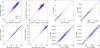 |
Fig. B.1. Differences between the STARLIGHT SSP fit between observed photometry spectra and photometry spectra that are scaled to the SDSS. Extensive parameters (mass, SFR) are shifted from the diagonal, and all other intensive parameters are very consistent. |
Appendix C: Measured and corrected parameters
Table C.1 is only available in electronic form at the CDS via anonymous ftp to cdsarc.u-strasbg.fr (130.79.128.5) or via http://cdsweb.u-strasbg.fr/cgi-bin/qcat?J/A+A/
All Tables
Results of the fifth-order polynomial fits to the fixed angular aperture corrections given in Iglesias-Páramo et al. (2013, 2016), in the form a0 + a1 * x + a2 * x2 + a3 * x3 + a4 * x4 + a5 * x5, where x is r/R50.
Results of the LINMIX MCMC slopes and the difference (steps) between the high and low bin.
Host galaxy redshifts used in this work that are different by more than 3% compared to those reported in the DR.
All Figures
|
Fig. 1. Distributions of scale factors for the 1066 spectra of our initial sample. Each distribution represents an SDSS filter. |
| In the text | |
|
Fig. 2. Spectrum of the SN2005ku (SDSS10805) host galaxy (black), together with the best STARLIGHT fit (red) and the pure nebular emission line spectrum (the difference is in blue). We note that this method accounts for the absorption produced at Balmer emission line positions. In-box panels contain the distributions of the percentual contribution of the SSP models used in the STARLIGHT fit, weighted to the mass (left) and the light (right) of the host galaxy. |
| In the text | |
|
Fig. 3. [O III]/Hβ vs. [N II]/Hα BPT diagram of the 869 galaxies with reliable emission lines. We excluded all 137 galaxies (in orange) that fall in the region above the line by Kewley et al. (2001), which determines that the underlying ionization source is not star formation but rather an AGN. |
| In the text | |
|
Fig. 4. SFR–M⋆, O/H–M⋆, and sSFR–M⋆ relations for our sample of galaxies. Star-forming (colored crosses) and composite (gray triangles) galaxies based on the BPT classification are represented in each diagram. The left and central panels correspond to Case A and Case B, respectively. We included the linear fit of the SFR–M⋆ relation for all the SF galaxies. The right panels correspond to Case C, with the aperture corrected. In the upper panel we include the linear fit of the SFR–M⋆ relation for all the SF galaxies considered in Case C (dashed red line), the fit from Case A (dotted green line), and the fit from Case B (dotted blue line). In the bottom-right panel, the sSFR–M⋆ relation, we also include a fourth relation (dotted red) that corresponds to an aperture-corrected SFR (Case C) normalized to the mass measured in the fiber spectrum (Case A). In the lower panels we show the difference between the linear fit in Case C and the linear fits of Case A (dotted green line) and Case B (dotted blue line). |
| In the text | |
|
Fig. 5. Distribution of the differences of the studied parameters among cases. Upper-left panel: histogram of the differences in SFR values for Cases C and A (red) and Cases C and B (blue). Upper-right panel: histogram of the differences in 12+log(O/H) values for Cases C and A (red) and Cases C and B (blue). Lower-left panel: histogram of the differences in sSFR values for Cases C and A (red), Cases C and B (blue), and with the SFR corrected but divided by the observed mass within the fiber (gray). Lower-right panel: histogram of the differences in |
| In the text | |
|
Fig. 6. Comparison between the remaining sample of galaxies once the g-band fraction or aperture correction criteria are considered. Left:g-band flux fraction covered within the fiber with respect to the total magnitude (“modelMag” in the SDSS catalogue) of the galaxy. The horizontal line at 0.2 corresponds to the cut suggested by Kewley et al. (2005) and used in D’Andrea et al. (2011) and Wolf et al. (2016) to justify that objects below the line on the shaded region have spectra that are not representative of the whole galaxy and therefore were excluded from those analyses. Middle:g-band fiber flux fraction vs. radii of the galaxy normalized to the Petrosian R50 radius (radius of a circle that contains 50% of the galaxy light). The horizontal line is the Kewley et al. (2005) limit, under which all objects (in the shaded region) would be excluded. The vertical line corresponds to the range where our aperture corrections are applied, and objects in the shaded region to the left (r/R50 < 0.3) are excluded because Iglesias-Páramo et al. (2013, 2016) corrections cannot be applied. We note that those galaxies with r/R50 ≥ 0.3 (to the right of the vertical line) but a g-band fiber flux fraction lower than 0.2 (below the horizontal line) would have been excluded but are included in this work. Right: normalized radii (r/R50) of the galaxies vs. redshift. Dots with black edges correspond to the 159 objects that we would have discarded using the g-band fraction criterion. In our selection we have mostly lost galaxies at low redshifts. |
| In the text | |
|
Fig. 7. g-band fraction (left column) and galaxy radius covered by the fiber in R50 units (right column) as a function of the main galaxy parameters used in this work: stellar mass, oxygen abundance, sSFR, and HαEW. The shadowed regions represent the regions excluded under each criterion. This figure clearly shows that under one criterion fewer objects are excluded, and it shows the tendency to exclude objects with higher or lower values for each galaxy parameter. |
| In the text | |
|
Fig. 8. x1 and c light-curve parameter and Hubble residual distributions of the full SDSS-II DR (green) compared to those of the samples after applying the fiber radius in R50 units (blue) and the g-band fraction (in red) cuts used here. Vertical colored lines represent the mean of the samples, and dashed black lines define the quality selection range. |
| In the text | |
|
Fig. 9. x1, c, and Hubble residual correlations with host galaxy parameters – stellar mass, oxygen abundance, sSFR, and HαEW – for the aperture-corrected sample (in blue) and the g-band fraction sample (in red). Solid transparent lines are the 10 000 individual slopes found with the LINMIX MCMC sampler, with the average slope as a solid line on top. Overplotted there are the average and standard deviation of the variable on the Y-axis in each of the two high and low bins in the X-axis variable, which has been divided using the median X value as the split point. The height of the box represents the error of the mean in each bin. |
| In the text | |
|
Fig. 10. SN Ia light-curve x1 and c parameters and Hubble residual dependences on stellar mass, oxygen abundance, sSFR, and HαEW of the 114 objects that are discarded using the g-band fraction criterion. Black lines represent the mean of the distribution, and red and blue lines represent the mean of the g-band fraction and aperture-corrected samples, respectively. Regarding light-curve parameters and Hubble residuals, while the three original distributions are centered at zero, these discarded objects have positive averages in the three distributions, leaving on average more negative biased distributions in the g-band fraction sample. Moreover, discarded objects have, on average, a larger stellar mass, lower HαEW, lower sSFR, and higher metallicity with respect the aperture-corrected sample, so the g-band fraction criterion also leaves a sample of SNe Ia and host galaxies that are biased toward the other side of the distributions. |
| In the text | |
|
Fig. 11. Cosmological constraints. Top: constraints on Ωm, ΩΛ when considering the aperture-corrected sample (blue), compared to the g-band fraction sample (red) and the entire SDSS sample (green). The best-fit value for the SDSS data set, assuming a flat ΛCDM model (plotted as a dashed black line) is shown as a black star. Differences in the contours are primarily due to different host galaxy selection. Bottom: 1D, marginalized contours for Ωm are shown for the three samples, once a flat ΛCDM cosmology is assumed. |
| In the text | |
|
Fig. 12. Visual extinction as a function of the main host galaxy parameters studied in this work. Blue and red symbols represent the aperture-corrected and the g-band fraction samples, respectively. The box widths represent the error of the mean, and the vertical lines represent the scatter in that bin. |
| In the text | |
|
Fig. B.1. Differences between the STARLIGHT SSP fit between observed photometry spectra and photometry spectra that are scaled to the SDSS. Extensive parameters (mass, SFR) are shifted from the diagonal, and all other intensive parameters are very consistent. |
| In the text | |
Current usage metrics show cumulative count of Article Views (full-text article views including HTML views, PDF and ePub downloads, according to the available data) and Abstracts Views on Vision4Press platform.
Data correspond to usage on the plateform after 2015. The current usage metrics is available 48-96 hours after online publication and is updated daily on week days.
Initial download of the metrics may take a while.