| Issue |
A&A
Volume 659, March 2022
|
|
|---|---|---|
| Article Number | A22 | |
| Number of page(s) | 12 | |
| Section | Interstellar and circumstellar matter | |
| DOI | https://doi.org/10.1051/0004-6361/202141537 | |
| Published online | 28 February 2022 | |
Magnetic field structure of OMC-3 in the far infrared revealed by SOFIA/HAWC+
University of Kiel, Institute of Theoretical Physics and Astrophysics,
Leibnizstrasse 15,
24118
Kiel,
Germany
e-mail: This email address is being protected from spambots. You need JavaScript enabled to view it.
Received:
14
June
2021
Accepted:
9
November
2021
Abstract
We report the SOFIA/HAWC+ band D (154 μm) and E (214 μm) polarimetric observations of the filamentary structure OMC-3 that is part of the Orion molecular cloud. The polarization pattern is uniform for both bands and parallel to the filament structure. The polarization degree decreases toward regions with high intensity for both bands, revealing a so called “polarization hole”. We identified an optical depth effect in which polarized emission and extinction act as counteracting mechanisms as a potential contributor to this phenomenon. Assuming that the detected polarization is caused by the emission of magnetically aligned non-spherical dust grains, the inferred magnetic field is uniform and oriented perpendicular to the filament. The magnetic field strength derived from the polarization patterns at 154 and 214 μm amounts to 202 and 261 μG, respectively. The derived magnetic field direction is consistent with that derived from previous polarimetric observations in the far infrared and submillimeter wavelength range. Investigating the far-infrared polarization spectrum derived from the SOFIA/HAWC+ observations, we do not find a clear correlation between the polarization spectrum and cloud properties, namely, the column density, N(H2), and temperature, T.
Key words: magnetic fields / polarization / techniques: polarimetric / ISM: magnetic fields / ISM: individual objects: OMC-3
© ESO 2022
1 Introduction
Magnetic fields in astrophysical objects are ubiquitous and can be found on both small and large scales. However, the role of magnetic fields in various physical processes, in particular, star formation, is matter of ongoing debate. For instance, magnetic fields are considered as a mechanism which slows down the contraction of star-forming regions and filaments, thus, providing a possible explanation for the low star formation rates that have been observed (Van Loo et al. 2015; Federrath 2015). Polarimetric oberservations of the thermal reemission radiation of magnetically aligned non-spherical dust grains can be used to derive the magnetic field structure and strength in star-forming environments.
It is assumed that radiative torque (RAT) alignment is the underlying process for aligning the dust grains. Here, elongated dust grains spin up and align with their longer axis perpendicular to the magnetic field lines due to the Barnett effect (Barnett 1915; Lazarian 2007; Lazarian & Hoang 2007; Hoang & Lazarian 2009) in the presence of an anisotropic radiation field (e.g., a central star embedded in a circumstellar envelope).
A broad range of attempts has been undertaken to detect this polarized radiation, such as with JCMT/SCUBA-2 (Holland et al. 2013), the Planck satellite (Planck Collaboration I 2011), and ALMA. In recent years, HAWC+ (Harper et al. 2018) aboard the Stratospheric Observatory for Infrared Astronomy (SOFIA) opened the far-infrared view for polarimetry. Using SOFIA/HAWC+, galaxies (Jones et al. 2020; Lopez-Rodriguez et al. 2020), Bok globules (Zielinski et al. 2021), prestellar cores (Redaelli et al. 2019) and filaments (Chuss et al. 2019) have been observed.
In the context of high-mass star formation, highly supercritical filaments are of particular interest. Using the Herschel Space Observatory (Pilbratt et al. 2010), filamentary structures in the interstellar medium have been detected (e.g., André et al. 2010; Schisano et al. 2020). These observational results agree well with the predictions from numerical studies, which are showing that the ISM should be highly filamentary on all scales and star formation is linked to self-gravitating filaments (see André et al. 2014, for a review of this topic). Understanding the physical properties of filaments is therefore crucial for understanding star formation in depth on galactic scales.
Since the Orion molecular cloud complex is the closest region that is undergoing massive star formation, it has been studied intensively. We present polarimetric observations of OMC-3, a star-forming region at a distance of 388 pc (Kounkel et al. 2017), which is part of the integral shape filament of the Orion molecular cloud. Several prestellar and protostellar sources have been identified in OMC-3 (Chini et al. 1997). The protostellar sources in this region include Class 0 and Class I protostars (e.g., Chini et al. 1997; Nielbock et al. 2003). MMS6 is the brightest source in OMC-3 with at least a factor of five larger flux density at (sub)millimeter wavelengths, as compared to all the other OMC-2/3 sources (Matthews et al. 2005; Takahashi et al. 2009). MMS6 has a bolometric luminosity of Lbol < 60 L⊙ and a core mass of Mcore = 30 M⊙ (Chini et al. 1997). Furthermore, multiple radio jets, molecular outflows, and shock-excited H2 emission have been detected (Yu et al. 1997; Reipurth et al. 1999; Aso et al. 2000; Stanke et al. 2002; Matthews et al. 2005). In particular, OMC-3 is a well-studied region with polarimetric observationsranging from the far infrared to submillimeter (submm) and millimeter (mm) wavelengths (e.g., Matthews et al. 2001; Houde et al. 2004; Takahashi et al. 2019; Liu 2021). SCUBA and Hertz polarimetric observations have revealed a highly ordered large-scale magnetic field for OMC-3, perpendicular to the filament. However, Takahashi et al. (2019) and Liu (2021) showed that the small-scale magnetic field has more complex structures using JVLA and ALMA observations. High-resolution polarimetric observations in the far-infrared enable further insights and restrictions of the properties of the magnetic field and the dust by, for instance, studying the polarization spectrum. The polarization spectrum, namely, the polarization degree as a function of wavelength, was first measured in the far-infrared by Hildebrand et al. (1999) using the Kuiper Airborne Observatory. Since then, a great deal of work has been carried out on the basis of observations (e.g., Vaillancourt et al. 2008; Vaillancourt & Matthews 2012; Gandilo et al. 2016)and theoretical frameworks (e.g., Bethell et al. 2007; Draine & Fraisse 2009; Guillet et al. 2018) in an effort to understand and interpret this quantity. Using the SOFIA/HAWC+ polarimeter, it is nowadays possible to study the polarization spectrum more precisely, that is, with higher angular resolution and sensitivity (e.g., Santos et al. 2019; Chuss et al. 2019). We report the polarimetric observations of OMC-3 at 154 and 214 μm obtained with SOFIA/HAWC+, which provide further insights into the magnetic field properties and the far-infrared polarization spectrum of this region of interest.
This paper is organized as follows. In Sect. 2, we describe the data acquisition and reduction and the selection criteria we apply to constrain the data. In Sect. 3, we present the polarization maps of OMC-3 and the corresponding analysis. We derive the magnetic field structure and strength of OMC-3 in Sect. 3.2. The relation between the polarization degree and the cloud properties is discussed in Sect. 3.3. Additionally, in Sect. 4, we provide a short discussion of our findings of the magnetic field structure in the context of complimentary polarimetric observations of this source. Finally, we summarize our results in Sect. 5.
2 Observations
Data aquisition
SOFIA/HAWC+ band D and E observations of OMC-3 were carried out on the 1st of October 2019 as part of the SOFIA Cycle 7 (Proposal 07_ 0026). Bands D and E provide an angular resolution of 13.6″ and 18.2″ full width at half maximum (FWHM) at the 154 and 214 μm center wavelength, respectively. The detector format consists of two 64 × 40 arrays, each comprising two 32 × 40 sub-arrays (Harper et al. 2018). The observations were performed using the chop-nod procedure with a chopping frequency of 10.2 Hz.
The raw data were processed by the HAWC+ instrument team using the data reduction pipeline version 2.3.0. This pipeline consists of different data processing steps including corrections for dead pixels as well as the intrinsic polarization of the instrument and telescope (for a brief description of all steps, see for instance Santos et al. 2019), resulting in “Level 4” (science-quality) data. These include FITS images of the total intensity (Stokes I), polarization degree p, polarization angle θ, Stokes Q and Stokes U, and all related uncertainties. The polarization degree p is calculatedvia
 (1)
(1)
Furthermore, to increase the reliability of our findings, we apply two additional criteria for the data that will be considered in the subsequent analysis:
 (2)
(2)
 (3)
(3)
where σI and σp are the standard deviations of I and p, respectively. In total, we obtained 1299 and 1710 Nyquist-sampled detections at 154 and 214 μm, respectively, which meet criteria Eqs. (2) and (3).
3 Results
3.1 Polarization map of OMC-3
The SOFIA/HAWC+ bands D and E have different fields-of-view, namely, 3.7′ × 4.6′, and 4.2′ × 6.2′ for bands D and E, respectively (Harper et al. 2018). Therefore, we focus on a region with valid polarization data for both bands, that is, polarization data meeting criteria Eqs. (2) and (3). Figure 1 shows the resulting band D (154 μm, left) and E (214 μm, right) polarization maps of OMC-3, overlaid on the corresponding intensity maps. The complete polarization maps for both wavelengths are shown in Fig. A.1.
Figure 2 shows the distribution of the polarization angles θ of OMC-3 for SOFIA/HAWC+ 154 μm (top) and 214 μm (bottom). We mostly find polarization angles ranging from −50° to −10° with clear predominance around −30° for both wavelengths.
In Fig. 3, the distribution of the polarization degree, p, is shown. For both wavelengths the degree of polarization varies between 0.5 and ~15%. The polarization degree is in general higher at 154 μm ( ± 2.7%) than at 214 μm (
 ± 2.0%).
A higher degree of polarization at a shorter wavelength is not expected, but can be explained by the fact that many polarization vectors at 154 μm in regions of higher intensity (lower degree of polarization) do not meet conditions in Eqs. (2) and (3). As a result, most of the polarization vectors are in low-intensity (higher degree of polarization) regions. If we only consider regions of higher intensity (e.g., I > 0.2 Imax), then the degree of polarization is smaller at 154 μm than at 214 μm ( ± 1.0%,
  ± 1.0%).
3.2 Magnetic field structure and strength
Assuming that the detected polarization is caused by the emission of magnetically aligned non-spherical dust grains, we can rotate the polarization angles by 90° to obtain the projection of the magnetic field direction integrated along the line-of-sight (henceforth, the magnetic field direction). The magnetic field of OMC-3 is visualized using the line-integral-convolution technique (LIC; Cabral & Leedom 1993, see Fig. 4). The intensity is displayed and color-coded, while the LIC textures represent the inferred magnetic field direction. For both wavelengths, the magnetic field direction is oriented perpendicular to the filament structure. This finding is similar to existing polarimetric observations of OMC-3 on similar scales (Matthews et al. 2001; Houde et al. 2004).
Refering to the Chandrasekhar-Fermi method (Chandrasekhar & Fermi 1953), we calculate the magnetic field strength of OMC-3 following Pattle et al. (2017). Here we are meant to assume that the underlying magnetic field is frozen in the cloud material. The plane-of-sky magnetic field strength (Bpos) can be calculated according to Crutcher et al. (2004):
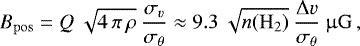 (4)
(4)
where σv represents the velocity dispersion, σθ the dispersion of the polarization angles, ρ the gas density, Δv the velocity dispersion in km s−1, n(H2) the numberdensity of molecular hydrogen, and Q = 0.5 (Crutcher et al. 2004) is a correction factor to account for variation of the field strength on scales smaller than the beam size. As the Chandrasekhar-Fermi method does not constrain the line-of-sight component of the magnetic field strength, the total magnetic field strength amounts to:
 (5)
(5)
For the subsequent analysis, we considered a rectangular area of OMC-3, centered on the point of maximum column density (see Sect 3.3): RA 5h35m20.5s, Dec −5°00′49″. The selected area has an angular width of 2′ 13.2″ and angular height of 1′ 36.2″, corresponding to 0.26 and 0.18 pc, respectively, at a distance of 388 pc (Kounkel et al. 2017).
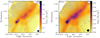 |
Fig. 1 SOFIA/HAWC+ band D (154 μm, left) and E (214 μm, right) polarization maps of OMC-3. The total intensity is shown with overlaid polarization vectors in blue. The length of the vectors is proportional to the polarization degree and the direction gives the orientation of the linear polarization. The isocontour lines mark 20, 40, 60, and 80% of the maximum intensity. According to criteria Eqs. (2) and (3), only vectors with I > 100 σI and p > 3 σp ought to be considered (see Sect. 2). The beam sizes of 13.6″ for 154 μm and 18.2″ for 214 μm (defined by the FWHM) are indicated in the lower right corners of their corresponding plots. |
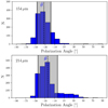 |
Fig. 2 Histograms showing the distribution of polarization angles of band D (154 μm, top) and band E (214 μm, bottom), respectively. The dashed lines represent the mean polarization angle
|


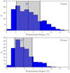 |
Fig. 3 Histograms showing the distribution of polarization degrees of band D (154 μm, top) and band E (214 μm, bottom), respectively. The dashed lines represent the mean polarization degree
|


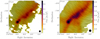 |
Fig. 4 SOFIA/HAWC+ intensity maps of OMC-3 at 154 (left) and 214 μm (right). Using the line-integral-convolution technique, the magnetic field direction is displayed. The isocontour lines mark 20, 40, 60, and 80% of the maximum intensity. According to criteria Eqs. (2) and (3), only vectors with I > 100 σI and p > 3 σp are considered (see Sect. 2). The beam sizes of 13.6″ at 154 μm and 18.2″ at 214 μm (defined by the FWHM) are indicated in the lower right. |
3.2.1 Volume density distribution of OMC-3
To calculate the magnetic field strength of OMC-3, we determine the volume density distribution, the velocity dispersion, and the dispersion of polarization angles.
In Sect. 3.3, we determine the column density across OMC-3 using a single temperature-modified blackbody fit. By using this fitting technique, which includes, among other things, the optical depth and the Planck function, the column density, the temperature, and the dust emissivity index can be derived. To calculate the volume density of OMC-3, we follow Pattle et al. (2017). We assume that OMC-3 is a cylindrical filament with a radius, r, and length, L. The volume then is πr2L and the above-mentioned rectangular area is the projection of that volume onto the plane of the sky, were the area is 2rL. The volume density amounts to:
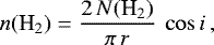 (6)
(6)
where i represents the inclination angle between filament and plane of sky. The inclination angle is unknown and we assume that the filament axis is oriented close to the plane of sky, meaning cos i ≈ 1. It should be noted that if the filament is tilted to the plane of sky, the volume density would decrease by a factor of  , if the inclination angle is 45°. Inside the considered area of OMC-3, we obtain a mean value of N(H2) = (1.71 ± 1.0) × 1022 cm−2. We determine the volume density as n(H2) = (3.82 ± 2.24) × 104 cm−3.
3.2.2 Velocity dispersion in OMC-3
Aso et al. (2000) observed the OMC-2/3 region in the H13CO+, HCO+ (1–0), and CO (1–0) lines using the Nobeyama 45 m radio telescope. We determined the velocity dispersion of the gas in OMC-3 using the H13CO+ observations, as shown in Table 2 in Aso et al. (2000). Here, several sources, namely AC2, AC3, AC4, are identified which are located within our considered area. The mean velocity dispersion amounts to σv = 0.983 ± 0.005 km s−1.
3.2.3 Dispersion of polarization angles
We calculated the standard devation of the mean polarization angles at 154 and 214 μm inside our considered area using the 95% confidence interval. We get σθ,D = 11.24 deg and σθ,E = 8.68
 deg. In Table 1, we provide an overview of the parameters in relation to the calculation of the magnetic field strength of OMC-3. Using these values, the corresponding plane-of-sky magnetic field strength amounts to 159 and 205 μG, derived from the 154 and 214 μm measurements, respectively. The total magnetic field strength amounts to 202 (154 μm) and 261 μG (214 μm). The calculated magnetic field strength values for OMC-3 are lower than the values derived for OMC-1 (300–1000 μG, Houde et al. 2009; Chuss et al. 2019). The difference can be traced back to the fact that the velocity dispersion for OMC-1 is higher (3.12 km s−1, Pattle et al. 2017). Our derived magnetic field strengths are similiar to 190 μG, reported by Poidevin et al. (2010) using 850 μm SCUBA data for OMC-3 MMS1-7.
Based on the derived magnetic field strength, we calculate the mass-to-flux ratio λ. We follow Crutcher et al. (2004) to obtain:
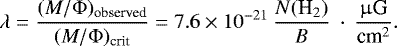 (7)
(7)
Here, N(H2) describes the column density and B the magnetic field strength. Using the derived values above, we obtain λ154 μm = 0.64 and λ214 μm = 0.49
 ; in particular, both measurements indicate that the filament is subcritical, similarly to OMC-1, where Pattle et al. (2017) derived a value of λOMC-1 = 0.41.
Overview of the properties in relation to the Chandrasekhar-Fermi method for the calculation of the magnetic field strength of OMC-3.
3.3 Correlation between magnetic field structures and cloud properties
In the following, we investigate how the polarization degree and angle, measured with SOFIA/HAWC+, change with cloud properties, namely, the column density and temperature. For this purpose, we follow Chuss et al. (2019) to construct column density, temperature, and dust emissivity maps.
Data preparation
In order to derive the column density, temperature, and dust emissivity maps, we used the SOFIA/HAWC+ 154 and 214 μm data, together with JCMT/SCUBA-21 850 μm and Herschel PACS2 70 and 160 μm data. We re-projected all data to the pixel scale of the measurement of 214 μm. In the next step, we beam-convolved the 70, 154, 160, and 850 μm data to the corresponding resolution of HAWC+ band E (214 μm) of 18.2″.
Fitting routine
We fit a single-temperature modified blackbody function to each pixel:
 (8)
(8)
Here, Bν(T) describes the Planck function and τν the optical depth:
 (9)
(9)
where the quantity β is the dust emissivity index and ν0 a reference frequency. The parameter ϵ is a scaling factor related to the column density N(H2):
 (10)
(10)
Here,  is the reference dust opacity per unit mass, mH the atomic mass of hydrogen, and μ the mean molecular weight per hydrogen atom. We set ν0 to 1000 Hz and adopt
  (1000 Hz) = 0.1 cm2 g−1. The final resulting fit function is:
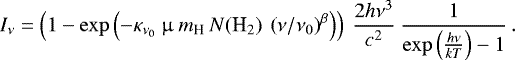 (11)
(11)
The fit parameters are the column density N(H2), the temperature T, and the dust emissivity index β. We adopted the uncertainties for the Stokes I data given in Chuss et al. (2019) and rejected all fitted pixels with a reduced χ2 (used to estimate the goodness of the fit) greater than 10. The resulting maps of column density, temperature, and dust emissivity index are shown in Fig. 5.
The dust emissivity index β is lowest at the central regions of OMC-3 and increases toward the outer regions, indicating potential dust grain growth at regions withhigher density and in the vicinity of stellar sources. The mean dust emissivity index amounts to  = 1.72. With this type of fitting technique, it is often omitted that beta is a free parameter (e.g., Gandilo et al. 2016; Santos et al. 2019). Santos et al. (2019) used a fixed value of β = 1.62 for ρ Oph A, while Gandilo et al. (2016) applied β = 2.0 for the Vela C molecular cloud. These fixed values are similar to our derived mean value.
In the maps shown in Fig. 5, we mark the known stellar sources (white/black star signs; from Chini et al. 1997). The embedded stellar sources radiate and heat the surrounding dust, that is, the position of stellar sources is closely connected to an increased temperature. The highest temperature can be found in the vicinity of MMS6, the most luminous source in OMC-3 (Matthews et al. 2005; Takahashi et al. 2009). The only exception where the presence of a stellar source is not related to an increased temperature, is MMS4 at RA: 5h 35m 20.5s, Dec: −5°0′53″. One possible explanation for this sole exception is the optical depth, which is highest at this stellar position (see Fig. B.1). The mean temperature is  = 28.38 K. The column density is highest around MMS4 with
  = 5.15 × 1022 cm−2. The mean column density amounts to
  = 1.10 × 1022 cm−2.
3.3.1 Degree of polarization as a function of the local column density
Polarimetricobservations of star-forming regions often show a decreasing degree of polarization with increasing density, making up so-called “polarization holes” (e.g., Henning et al. 2001; Wolf et al. 2003; Chuss et al. 2019; Zielinski et al. 2021). We investigate how the polarization degree changes in relation to the column density derived above. As in the data preparation shown in Sect. 3.3, the Stokes parameter Q and U at 154 μm are re-projected and beam-convolved to 214 μm resolution as well. The polarization degree is then calculated using
 (12)
(12)
Our results for 154 and 214 μm are shown in Fig. 6.
For both wavelengths, the polarization degree decreases from ~10 to ≲1% with increasing density. Inspired by the work of Davis et al. (2000), who applied linear least-square fits to polarimetric observationsof the Serpens cloud core and found a correlation between the measured polarization and intensity, Henning et al. (2001) found a correlation between these quantities in the case of the two Bok globules CB54 and DC253-1.6 as well. They approximated the decrease in the polarization degree as a function of increasing intensity using the following equation:
 (13)
(13)
where a0, a1, and a2 are fitting parameters. We applied the same technique, but refer to the column density instead of intensity. If we assume that the dust distribution is optically thin, the intensity is connected to the density. Therefore, the subsequent results are comparable. For our case we apply
 (14)
(14)
We obtained a0,154 μm = −0.53 ± 0.24, a1,154 μm = 1.58 ± 0.20, a2,154 μm = −0.51 ± 0.04 and a0,214 μm = 0.44 ± 0.16, a1,214 μm = 0.81 ± 0.12, a2,214 μm = −0.63 ± 0.05. The parameter a2, which describes the slope of the curve, is slightly higher at 214 μm. Interestingly, comparing this slope to those reported in the previous studies for Bok globules, a different object class, one can see that the slopes are similar. For the Bok globule B335, Wolf et al. (2003) derived a2,850 μm = −0.43 with JCMT/SCUBA and Zielinski et al. (2021) derived a2,214 μm = −0.55 with SOFIA/HAWC+. Furthermore, the calculated slope for the Bok globule CB54 is a2,850 μm = −0.64 (Henning et al. 2001)and a2,850 μm = −0.55 for DC 253-1.6 (Henning et al. 2001). See Table 2 for an overview of all calculated a2 values. There are multiple possible reasons for the occurence of polarization holes. Since the slope is similar for different object classes and wavelengths, this may be a hint that the same effects are responsible. However, this needs further investigation, since the spatial scale on which the polarization hole in OMC-3 is examined is larger than that of the Bok Globule studies mentioned above.
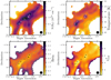 |
Fig. 5 Maps of column density (top left), temperature (top right), dust emissivity index (bottom left), and the corresponding reduced χ2 (bottom right). The beam size of 18.2″ (band E, 214 μm) is indicated in the lower right for each figure. |
3.3.2 Polarization hole in OMC-3
The SOFIA/HAWC+ observations show a decrease of the polarization degree toward dense regions of OMC-3. As mentioned above, thereare several existing hypotheses that are aimed at explaining this phenomenon, such as an insufficient angular resolution ofa possibly complex magnetic field structure on scales below the resolution of the polarization maps (e.g., Shu et al. 1987; Wolf et al. 2004), a disruption of spinning larger grains into smaller fragments (radiative torque disruption, Hoang et al. 2019; Hoang 2019), or certain combinations of optical depth, dust grain size, and chemical composition(Brauer et al. 2016). What is particulaly interesting for our purposes is the latter proposal. Brauer et al. (2016) showed that a polarization hole can occur as a result of the superposition of polarized emission and dichroic extinction, which act as counteracting mechanisms. This effect may even cause a flip in the polarization direction by 90°, if the dichroic extinction dominates over dichroic emission (Reissl et al. 2014; Brauer et al. 2016). Indeed, Liu (2021) showed this 90° flip for OMC-3 (MMS6) with a comparison of 1.2 mm ALMA and 9 mm JVLA polarimetric observations, see Fig. 7. They find that the innermost ~100 au region of OMC-3 (MMS6) is optically thick at 1.2 mm and optically thin at 9 mm.
Given a moderate optical depth, the counteracting mechanisms of polarized emission and absorption result in a decrease of the polarization degree. However, this effect can only be applied to explain the polarization hole in the innermost area of OMC-3. The reason for the decrease in the degree of polarization in the outer areas is unknown. The polarimetric ALMA observation shows that the magnetic field in OMC-3 is more complex on smaller scales. Due to beam-averaging, an unresolved and more complex magnetic field would lead to a lower degree of polarization. While the optical depth seems to have an effect on the decrease in the polarization degree, we cannot rule out a potential influence of the magnetic field complexity. However, other effects, such as the radiative torque disruption (Hoang et al. 2019; Hoang 2019) or less-aligned dust grains at higher densities (Goodman et al. 1992; Creese et al. 1995), along with their contribution to the polarization hole, cannot be ruled out.
Calculated values for the parameter a2 that describes the slope of the polarization hole at different wavelengths.
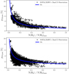 |
Fig. 6 Polarization degree at 154 (top) and 214 μm (bottom) as a function of the column density, scaled to the maximum value. |
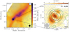 |
Fig. 7 OMC-3 polarization maps at different scales. Left: total intensity is shown with overlaid polarization vectors in blue. The length of the vectors is proportional to the polarization degree and the direction gives the orientation of the linear polarization. Right: total intensity, observed at 1.2 mm with ALMA, is shown with overlaid polarization vectors in blue. Red polarization vectors are oberserved with JVLA at 9 mm (Liu 2021, ©AAS. Reproduced with permission). |
3.3.3 Degree of polarization versus temperature
In Fig. 8, we show the obtained polarization degrees at 154 and 214 μm as a function of the derived temperature. The temperature is strongly correlated with the position of stars. The degree of polarization drops sharply in the vicinity of the stars, while the degree of polarization is higher in colder regions.
3.3.4 Polarization spectrum versus column density and temperature
In the next step, we investigate how the polarization spectrum, that is, the polarization degree as a function of wavelength, changes with column density and temperature of OMC-3. We define the polarization spectrum as p214 μm∕p154 μm, similiar to Santos et al. (2019), who studied the polarization spectrum of ρ Oph A and Michail et al. (2021), who studied the polarization spectrum of OMC-1. Using this definition, p214 μm∕p154 μm < 1 indicates a negative spectral slope and p214 μm∕p154 μm > 1 a positive spectral slope. We calculated the polarization spectrum for all pixels where we have valid data for the polarization degrees at both wavelengths, namely, those data meeting criteria Eqs. (2) and (3), and valid data for the column density and temperature.
The spatially resolved map of p214 μm∕p154 μm is shown in Fig. 9. In the southern and eastern part of OMC-3, the polarization spectrum is smaller than 1, while in the central and northern part the spectrum is mostly greater than 1. The ratio of p214 μm∕p154 μm versus column density and temperature is shown in Figs. 10 (top and bottom), respectively. In our maps, we find a slightly larger number of data points with a negative slope (878) than with a positive slope (709). The mean polarization slope is slightly negative 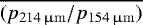 = 0.93 ± 0.24, indicating a relatively flat slope of the polarization spectrum. We do not find a clear correlation between polarization spectrum and column density. However, it does appear that the polarization spectrum is particularly flat (~1) at higher column densities (see Fig. 10 top). The polarization spectrum is smaller than 1 for low (≲25 K) and high (≳42 K) temperatures. However, in these cases the sample size is small if compared to the total number of data points. Therefore, no significant conclusion about the connection between the polarization ratio and the derived temperature is possible.
In contrast, Michail et al. (2021) find a positive correlation between the slope of the polarization spectrum and the temperatureof OMC-1. However, they report no significant correlation between slope and column density. In contrast, Santos et al. (2019) report a clear correlation between polarization spectrum and column density and temperature in ρ Oph A.
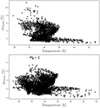 |
Fig. 8 Polarization degree at 154 (top) and 214 μm (bottom) as a function of the temperature. |
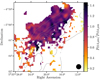 |
Fig. 9 Polarization spectrum (p214 μm∕p154 μm) map of OMC-3. The isocontour lines mark 10, 30, 50, 70, and 90% of the maximum column density. The beam size of 18.2″ at 214 μm (defined by the FWHM) is indicated in the lower right. |
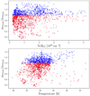 |
Fig. 10 Polarization spectrum (p214 μm∕p154 μm) versus column density (top) and temperature (bottom). Red (blue) crosses indicate a polarization spectrum smaller than 1 (larger than 1). |
4 Magnetic field of OMC-3 derived from observations in different wavelength ranges
OMC-3 is a well studied object with polarimetic observations ranging from the far-infrared to submm and mm. In the following, we compare these observations to the SOFIA/HAWC+ observation at 154 and 214 μm (see Fig. 11).
350 μm
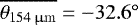
Houde et al. (2004) observed OMC-3 with SHARC II/Hertz at 350 μm. These authors reported a mean polarization angle of  = −43° ± 9° for OMC-3 MM1-6. If we limit our observations to the same region, we obtain
  = −34° ± 12° and
  = −34° ± 10° at 154 and 214 μm, respectively. The Stokes averaged polarization degree at 350 μm amounts to
  = 1.55% ± 0.12%. For the same region we obtain
  = 3.2% ± 1.71% and
  = 2.86% ± 1.35%. While the polarization angles are well aligned at 154, 214, and 350 μm, the polarization degree is 1–2% lower at 350 μm. The rather small standard deviation of the polarization degree at 350 μm indicates that here the polarization hole is not as prominent as it is at 154 and 214 μm.
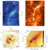 |
Fig. 11 Multiwavelength, multiscale polarization maps of OMC-3. Top left: intensity and polarization map obtained with SHARC II and Hertz at 350 μm, respectively. Overlaid are polarization vectors in white and black (Houde et al. 2004, ©AAS. Reproduced with permission). Top right: total intensity, observed at 850 μm with SCUBA, is shown with overlaid polarization vectors in blue (Matthews et al. 2001, ©AAS. Reproduced with permission). Bottom left: total intensity, observed at 1.2 mm with ALMA, is shown with overlaid polarization vectors in blue. Red polarization vectors are oberserved with JVLA at 9 mm (Liu 2021, ©AAS. Reproduced with permission). Bottom right: Total intensity, observed at 214 μm with SOFIA/HAWC+, is shown with overlaid polarization vectors in blue. |
850 μm
Matthews et al. (2001) observed OMC-3 with JCMT/SCUBA at 850 μm. The reported polarization angles are well aligned with our results. The mean polarization degree at 850 μm is 5.0%, including the observation at the southern regions (MMS7-10, see Fig. 11, top-right). This mean polarization degree is similar to our results, 4.8 ± 2.7 and 3.8 ± 2.0% for 154 and 214 μm, respectively. The 850 μm observation shows a polarization hole for OMC-3 as well.
1.2 and 9 mm
Liu (2021) observed OMC-3 with ALMA/JVLA at 1.2 and 9 mm. These high-resolution observations show that the polarization angles have a more complex pattern at small scales than they have at larger scales. Since SOFIA/HAWC+ does not allow resolving these structures, we do not compare the polarization degrees.
The magnetic field structure, which is derived from the SOFIA/HAWC+ observations, is consistent with the magnetic field, which was reported from previous polarimetric observations in the far infrared and submm wavelength range. While the magnetic field appears uniform at larger scales, it shows a a greater level of complexity on small scales.
5 Conclusions
We investigated the magnetic field of OMC-3 based on polarimetric observations with SOFIA/HAWC+ at 154 and 214 μm.
- 1.
The polarization maps of OMC-3 at 154 (band D) and 214 μm (band E) show a uniform pattern, parallel to the filament for both wavelengths. The mean polarization angles are
 ± 14.5°
and
± 14.5°
and  ± 20.4°
for 154 and 214 μm, respectively. These results are consistent with previous polarimetric observations of OMC-3 in the far-infrared and submm wavelength range (Matthews et al. 2001; Houde et al. 2004).
± 20.4°
for 154 and 214 μm, respectively. These results are consistent with previous polarimetric observations of OMC-3 in the far-infrared and submm wavelength range (Matthews et al. 2001; Houde et al. 2004). - 2.
The mean polarization degree amounts to
 ± 2.7% and
  ± 2.0% at 154 and 214 μm, respectively. The polarization degree decreases for both wavelengths toward regions with increased column density. An unequivocal explanation for the occurence of this “polarization hole” could not be found. However, the “optical depth effect”, namely, the superposition of polarized emission and dichroic extinction seems to be of importance in the innermost densest regions, consistent with the observed 90°
flip of the polarization vectors that has been observed using ALMA and JVLA.
± 2.0% at 154 and 214 μm, respectively. The polarization degree decreases for both wavelengths toward regions with increased column density. An unequivocal explanation for the occurence of this “polarization hole” could not be found. However, the “optical depth effect”, namely, the superposition of polarized emission and dichroic extinction seems to be of importance in the innermost densest regions, consistent with the observed 90°
flip of the polarization vectors that has been observed using ALMA and JVLA. - 3.
The magnetic field of OMC-3 is uniform and perpendicular to the filament for both wavelengths. We calculated a magnetic field strength of 202 μG at 154 μm and 261 μG at 214 μm.
- 4.
We do not find a general correlation between the polarization spectrum (p214 μm∕p154 μm) and cloud properties, that is, column density N(H2) and temperature T. These results are in contrast to previous studies of similar objects (Santos et al. 2019; Michail et al. 2021).
- 5.
The large-scale magnetic field structure and strength are consistently derived from observations that cover a wide range of wavelengths, that is, the far infrared to submm. On small scales, the magnetic field appears to be more complex.
Using SOFIA/HAWC+ we obtained new multiwavelength polarimetric observations of the filamentary structure OMC-3 at 154 and 214 μm. These observations reveal a uniform magnetic field, which is oriented perpendicular to the filament. These findings are in good agreement with previous observations at similar scale. No correlation between the polarization spectrum and cloud properties of OMC-3 has been found.
Acknowledgements
We thank Stefan Heese for data aquisition. This paper is based on observations made with the NASA/DLR Stratospheric Observatory for Infrared Astronomy (SOFIA). SOFIA is jointly operated by the Universities Space Research Association, Inc. (USRA), under NASA contract NNA17BF53C, and the Deutsches SOFIA Institut (DSI) under DLR contract 50 OK 0901 to the University of Stuttgart. Acknowledgement: N.Z. and S.W. acknowledge the support by the DLR/BMBF grant 50OR1910. The LIC code is ported from publically-available IDL source by Diego Falceta-Gonçalves.
Appendix A Polarization map of OMC-3
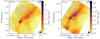 |
Fig. A.1 Complete SOFIA/HAWC+ band D (154 μm, left) and E (214 μm, right) polarization maps of OMC-3. The total intensity is shown with overlaid polarization vectors in blue. The length of the vectors is proportional to the polarization degree and the direction gives the orientation of the linear polarization. The isocontour lines mark 20, 40, 60, and 80% of the maximum intensity. According to criteria (2) and (3) only vectors with I > 100 σI and p > 3 σp are considered (see Sect. 2). The beam size of 13.6″ for band D and 18.2″ for band E (defined by the FWHM) are indicated on the lower-right. |
Appendix B Optical depth map of OMC-3 at 154, 160, 214, and 850 μm
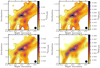 |
Fig. B.1 Maps of optical depth at wavelengths of 154 μm (top left), 160 μm (top right), 214 μm (bottom left), and 850 μm (bottom right). The contour lines mark 10, 20, 30, 40, 50, 60, 70, 80, and 90 % of the maximum optical depth for each wavelength. The white asterisk symbols mark known stellar sources (Chini et al. 1997). The beam size of 18.2″ (band E) is indicated on the lower-right of each figure. |
References
- André, P., Men’shchikov, A., Bontemps, S., et al. 2010, A&A, 518, L102 [NASA ADS] [CrossRef] [EDP Sciences] [Google Scholar]
- André, P., Di Francesco, J., Ward-Thompson, D., et al. 2014, in Protostars and Planets VI, ed. H. Beuther, R. S. Klessen, C. P. Dullemond, & T. Henning, 27 [Google Scholar]
- Aso, Y., Tatematsu, K., Sekimoto, Y., et al. 2000, ApJS, 131, 465 [NASA ADS] [CrossRef] [Google Scholar]
- Barnett, S. J. 1915, Phys. Rev., 6, 239 [CrossRef] [Google Scholar]
- Bethell, T. J., Chepurnov, A., Lazarian, A., & Kim, J. 2007, ApJ, 663, 1055 [NASA ADS] [CrossRef] [Google Scholar]
- Brauer, R., Wolf, S., & Reissl, S. 2016, A&A, 588, A129 [NASA ADS] [CrossRef] [EDP Sciences] [Google Scholar]
- Cabral, B., & Leedom, L. C. 1993, in Proceedings of the 20th annual conference on Computer graphics and interactive techniques, SIGGRAPH ’93 (New York, NY, USA: ACM), 263 [CrossRef] [Google Scholar]
- Chandrasekhar, S., & Fermi, E. 1953, ApJ, 118, 116 [Google Scholar]
- Chini, R., Reipurth, B., Ward-Thompson, D., et al. 1997, ApJ, 474, L135 [NASA ADS] [CrossRef] [Google Scholar]
- Chuss, D. T., Andersson, B. G., Bally, J., et al. 2019, ApJ, 872, 187 [Google Scholar]
- Creese, M., Jones, T. J., & Kobulnicky, H. A. 1995, AJ, 110, 268 [NASA ADS] [CrossRef] [Google Scholar]
- Crutcher, R. M., Nutter, D. J., Ward-Thompson, D., & Kirk, J. M. 2004, ApJ, 600, 279 [Google Scholar]
- Davis, C. J., Chrysostomou, A., Matthews, H. E., Jenness, T., & Ray, T. P. 2000, ApJ, 530, L115 [NASA ADS] [CrossRef] [Google Scholar]
- Draine, B. T., & Fraisse, A. A. 2009, ApJ, 696, 1 [Google Scholar]
- Federrath, C. 2015, MNRAS, 450, 4035 [Google Scholar]
- Gandilo, N. N., Ade, P. A. R., Angilè, F. E., et al. 2016, ApJ, 824, 84 [Google Scholar]
- Goodman, A. A., Jones, T. J., Lada, E. A., & Myers, P. C. 1992, ApJ, 399, 108 [Google Scholar]
- Guillet, V., Fanciullo, L., Verstraete, L., et al. 2018, A&A, 610, A16 [NASA ADS] [CrossRef] [EDP Sciences] [Google Scholar]
- Harper, D. A., Runyan, M. C., Dowell, C. D., et al. 2018, J. Astron. Instrum., 7, 1840008 [Google Scholar]
- Henning, T., Wolf, S., Launhardt, R., & Waters, R. 2001, ApJ, 561, 871 [NASA ADS] [CrossRef] [Google Scholar]
- Hildebrand, R. H., Dotson, J. L., Dowell, C. D., Schleuning, D. A., & Vaillancourt, J. E. 1999, ApJ, 516, 834 [NASA ADS] [CrossRef] [Google Scholar]
- Hoang, T. 2019, ApJ, 876, 13 [NASA ADS] [CrossRef] [Google Scholar]
- Hoang, T., & Lazarian, A. 2009, ApJ, 695, 1457 [NASA ADS] [CrossRef] [Google Scholar]
- Hoang, T., Tram, L. N., Lee, H., & Ahn, S.-H. 2019, Nat. Astron., 3, 766 [Google Scholar]
- Holland, W. S., Bintley, D., Chapin, E. L., et al. 2013, MNRAS, 430, 2513 [Google Scholar]
- Houde, M., Dowell, C. D., Hildebrand, R. H., et al. 2004, ApJ, 604, 717 [NASA ADS] [CrossRef] [Google Scholar]
- Houde, M., Vaillancourt, J. E., Hildebrand, R. H., Chitsazzadeh, S., & Kirby, L. 2009, ApJ, 706, 1504 [Google Scholar]
- Jones, T. J., Kim, J.-A., Dowell, C. D., et al. 2020, AJ, 160, 167 [NASA ADS] [CrossRef] [Google Scholar]
- Kounkel, M., Hartmann, L., Loinard, L., et al. 2017, ApJ, 834, 142 [Google Scholar]
- Lazarian, A. 2007, J. Quant. Spectr. Rad. Transf., 106, 225 [Google Scholar]
- Lazarian, A., & Hoang, T. 2007, MNRAS, 378, 910 [Google Scholar]
- Liu, H. B. 2021, ApJ, 914, 25 [NASA ADS] [CrossRef] [Google Scholar]
- Lopez-Rodriguez, E., Dowell, C. D., Jones, T. J., et al. 2020, ApJ, 888, 66 [NASA ADS] [CrossRef] [Google Scholar]
- Matthews, B. C., Wilson, C. D., & Fiege, J. D. 2001, ApJ, 562, 400 [NASA ADS] [CrossRef] [Google Scholar]
- Matthews, B. C., Lai, S.-P., Crutcher, R. M., & Wilson, C. D. 2005, ApJ, 626, 959 [NASA ADS] [CrossRef] [Google Scholar]
- Michail, J. M., Ashton, P. C., Berthoud, M. G., et al. 2021, ApJ, 907, 46 [NASA ADS] [CrossRef] [Google Scholar]
- Nielbock, M., Chini, R., & Müller, S. A. H. 2003, A&A, 408, 245 [NASA ADS] [CrossRef] [EDP Sciences] [Google Scholar]
- Pattle, K., Ward-Thompson, D., Berry, D., et al. 2017, ApJ, 846, 122 [Google Scholar]
- Pilbratt, G. L., Riedinger, J. R., Passvogel, T., et al. 2010, A&A, 518, L1 [NASA ADS] [CrossRef] [EDP Sciences] [Google Scholar]
- Planck Collaboration I. 2011, A&A, 536, A1 [NASA ADS] [CrossRef] [EDP Sciences] [Google Scholar]
- Poidevin, F., Bastien, P., & Matthews, B. C. 2010, ApJ, 716, 893 [NASA ADS] [CrossRef] [Google Scholar]
- Redaelli, E., Alves, F. O., Santos, F. P., & Caselli, P. 2019, A&A, 631, A154 [NASA ADS] [CrossRef] [EDP Sciences] [Google Scholar]
- Reipurth, B., Rodríguez, L. F., & Chini, R. 1999, AJ, 118, 983 [NASA ADS] [CrossRef] [Google Scholar]
- Reissl, S., Wolf, S., & Seifried, D. 2014, A&A, 566, A65 [NASA ADS] [CrossRef] [EDP Sciences] [Google Scholar]
- Santos, F. P., Chuss, D. T., Dowell, C. D., et al. 2019, ApJ, 882, 113 [NASA ADS] [CrossRef] [Google Scholar]
- Schisano, E., Molinari, S., Elia, D., et al. 2020, MNRAS, 492, 5420 [Google Scholar]
- Shu, F. H., Adams, F. C., & Lizano, S. 1987, ARA&A, 25, 23 [Google Scholar]
- Stanke, T., McCaughrean, M. J., & Zinnecker, H. 2002, A&A, 392, 239 [NASA ADS] [CrossRef] [EDP Sciences] [Google Scholar]
- Takahashi, S., Ho, P. T. P., Tang, Y.-W., Kawabe, R., & Saito, M. 2009, ApJ, 704, 1459 [NASA ADS] [CrossRef] [Google Scholar]
- Takahashi, S., Machida, M. N., Tomisaka, K., et al. 2019, ApJ, 872, 70 [NASA ADS] [CrossRef] [Google Scholar]
- Vaillancourt, J. E., & Matthews, B. C. 2012, ApJS, 201, 13 [NASA ADS] [CrossRef] [Google Scholar]
- Vaillancourt, J. E., Dowell, C. D., Hildebrand, R. H., et al. 2008, ApJ, 679, L25 [NASA ADS] [CrossRef] [Google Scholar]
- Van Loo, S., Tan, J. C., & Falle, S. A. E. G. 2015, ApJ, 800, L11 [NASA ADS] [CrossRef] [Google Scholar]
- Wolf, S., Launhardt, R., & Henning, T. 2003, ApJ, 592, 233 [NASA ADS] [CrossRef] [Google Scholar]
- Wolf, S., Launhardt, R., & Henning, T. 2004, Ap&SS, 292, 239 [NASA ADS] [CrossRef] [Google Scholar]
- Yu, K. C., Bally, J., & Devine, D. 1997, ApJ, 485, L45 [NASA ADS] [CrossRef] [Google Scholar]
- Zielinski, N., Wolf, S., & Brunngräber, R. 2021, A&A, 645, A125 [NASA ADS] [CrossRef] [EDP Sciences] [Google Scholar]
Observation ID scuba2_00015_20180906T152402.
Observation IDs 1342204250, 1342204251.
All Tables
Overview of the properties in relation to the Chandrasekhar-Fermi method for the calculation of the magnetic field strength of OMC-3.
Calculated values for the parameter a2 that describes the slope of the polarization hole at different wavelengths.
All Figures
|
Fig. 1 SOFIA/HAWC+ band D (154 μm, left) and E (214 μm, right) polarization maps of OMC-3. The total intensity is shown with overlaid polarization vectors in blue. The length of the vectors is proportional to the polarization degree and the direction gives the orientation of the linear polarization. The isocontour lines mark 20, 40, 60, and 80% of the maximum intensity. According to criteria Eqs. (2) and (3), only vectors with I > 100 σI and p > 3 σp ought to be considered (see Sect. 2). The beam sizes of 13.6″ for 154 μm and 18.2″ for 214 μm (defined by the FWHM) are indicated in the lower right corners of their corresponding plots. |
| In the text | |
|
Fig. 2 Histograms showing the distribution of polarization angles of band D (154 μm, top) and band E (214 μm, bottom), respectively. The dashed lines represent the mean polarization angle
|
| In the text | |
|
Fig. 3 Histograms showing the distribution of polarization degrees of band D (154 μm, top) and band E (214 μm, bottom), respectively. The dashed lines represent the mean polarization degree
|
| In the text | |
|
Fig. 4 SOFIA/HAWC+ intensity maps of OMC-3 at 154 (left) and 214 μm (right). Using the line-integral-convolution technique, the magnetic field direction is displayed. The isocontour lines mark 20, 40, 60, and 80% of the maximum intensity. According to criteria Eqs. (2) and (3), only vectors with I > 100 σI and p > 3 σp are considered (see Sect. 2). The beam sizes of 13.6″ at 154 μm and 18.2″ at 214 μm (defined by the FWHM) are indicated in the lower right. |
| In the text | |
|
Fig. 5 Maps of column density (top left), temperature (top right), dust emissivity index (bottom left), and the corresponding reduced χ2 (bottom right). The beam size of 18.2″ (band E, 214 μm) is indicated in the lower right for each figure. |
| In the text | |
|
Fig. 6 Polarization degree at 154 (top) and 214 μm (bottom) as a function of the column density, scaled to the maximum value. |
| In the text | |
|
Fig. 7 OMC-3 polarization maps at different scales. Left: total intensity is shown with overlaid polarization vectors in blue. The length of the vectors is proportional to the polarization degree and the direction gives the orientation of the linear polarization. Right: total intensity, observed at 1.2 mm with ALMA, is shown with overlaid polarization vectors in blue. Red polarization vectors are oberserved with JVLA at 9 mm (Liu 2021, ©AAS. Reproduced with permission). |
| In the text | |
|
Fig. 8 Polarization degree at 154 (top) and 214 μm (bottom) as a function of the temperature. |
| In the text | |
|
Fig. 9 Polarization spectrum (p214 μm∕p154 μm) map of OMC-3. The isocontour lines mark 10, 30, 50, 70, and 90% of the maximum column density. The beam size of 18.2″ at 214 μm (defined by the FWHM) is indicated in the lower right. |
| In the text | |
|
Fig. 10 Polarization spectrum (p214 μm∕p154 μm) versus column density (top) and temperature (bottom). Red (blue) crosses indicate a polarization spectrum smaller than 1 (larger than 1). |
| In the text | |
|
Fig. 11 Multiwavelength, multiscale polarization maps of OMC-3. Top left: intensity and polarization map obtained with SHARC II and Hertz at 350 μm, respectively. Overlaid are polarization vectors in white and black (Houde et al. 2004, ©AAS. Reproduced with permission). Top right: total intensity, observed at 850 μm with SCUBA, is shown with overlaid polarization vectors in blue (Matthews et al. 2001, ©AAS. Reproduced with permission). Bottom left: total intensity, observed at 1.2 mm with ALMA, is shown with overlaid polarization vectors in blue. Red polarization vectors are oberserved with JVLA at 9 mm (Liu 2021, ©AAS. Reproduced with permission). Bottom right: Total intensity, observed at 214 μm with SOFIA/HAWC+, is shown with overlaid polarization vectors in blue. |
| In the text | |
|
Fig. A.1 Complete SOFIA/HAWC+ band D (154 μm, left) and E (214 μm, right) polarization maps of OMC-3. The total intensity is shown with overlaid polarization vectors in blue. The length of the vectors is proportional to the polarization degree and the direction gives the orientation of the linear polarization. The isocontour lines mark 20, 40, 60, and 80% of the maximum intensity. According to criteria (2) and (3) only vectors with I > 100 σI and p > 3 σp are considered (see Sect. 2). The beam size of 13.6″ for band D and 18.2″ for band E (defined by the FWHM) are indicated on the lower-right. |
| In the text | |
|
Fig. B.1 Maps of optical depth at wavelengths of 154 μm (top left), 160 μm (top right), 214 μm (bottom left), and 850 μm (bottom right). The contour lines mark 10, 20, 30, 40, 50, 60, 70, 80, and 90 % of the maximum optical depth for each wavelength. The white asterisk symbols mark known stellar sources (Chini et al. 1997). The beam size of 18.2″ (band E) is indicated on the lower-right of each figure. |
| In the text | |
Current usage metrics show cumulative count of Article Views (full-text article views including HTML views, PDF and ePub downloads, according to the available data) and Abstracts Views on Vision4Press platform.
Data correspond to usage on the plateform after 2015. The current usage metrics is available 48-96 hours after online publication and is updated daily on week days.
Initial download of the metrics may take a while.