| Issue |
A&A
Volume 659, March 2022
|
|
|---|---|---|
| Article Number | A130 | |
| Number of page(s) | 18 | |
| Section | Extragalactic astronomy | |
| DOI | https://doi.org/10.1051/0004-6361/202141043 | |
| Published online | 17 March 2022 | |
Tracing the outflow kinematics in Type 2 active galactic nuclei
1
Astronomical Observatory, Volgina 7, 11060 Belgrade, Serbia
e-mail: jkovacevic@aob.bg.ac.rs
2
Faculty of Physics, University of Belgrade, Studentski Trg 12, Belgrade, Serbia
3
Faculty of Mathematics, University of Belgrade, Studentski Trg 16, Belgrade, Serbia
Received:
10
April
2021
Accepted:
13
December
2021
We used a sample of 577 spectra of active galactic nuclei Type 1.8-2 (z < 0.25) taken from the Sloan Digital Sky Survey to trace the influence of the outflow kinematics on the profiles of different emission lines (Hβ, [O III], Hα, [N II], [S II]). All considered lines were fitted with two Gaussian components: one that fits the core of the line, and another that fits the wings. We provide a procedure for decomposition of the Hα+[N II] wavelength band for spectra where these lines overlap. The influence of the gravitational and non-gravitational kinematics on the line components is investigated by comparing the dispersions of the line components with stellar velocity dispersion. We find that wing components of all the considered emission lines have pure non-gravitational kinematics. The core components are consistent with gravitational kinematics for the Hα, [N II], and [S II] lines, while in the [O III] there is evidence for contribution from non-gravitational kinematics. We adopted the wing components as a proxy for the outflow contribution and investigated the outflow kinematics by analysing the correlations between the widths and shifts of the wing components of different lines. For this purpose, we used the subsets in which wing components are detected in both compared lines, and can be fitted independently. We find strong correlations between wing component shifts, as well as between wing component widths of all considered lines, with the exception of the Hβ wing component width. These correlations indicate that outflow dynamics systemically affect all emission lines in the spectrum. However, it reflects with a different strength in their profiles, which is observed as different widths of the wing components. This is investigated by comparison of the mean widths of the wing components in subsets where wing components are present in all lines. The strongest outflow signature is observed in the [O III] lines, which have the broadest wing components; weaker outflow signatures are found in Hα and [N II], and the weakest is found for [S II]. These results imply that the considered lines arise in different parts of an outflowing region.
Key words: galaxies: active / galaxies: Seyfert / quasars: emission lines / line: profiles
© ESO 2022
1. Introduction
Active galactic nuclei (AGNs) are one of the most powerful energy sources in the Universe. The enormous amount of energy radiated from the central source of an AGN is formed by the process of accretion around a super-massive black hole (SMBH), which is followed by the fast motion of the emitting gas and appearance of outflows. The large-scale phenomena, namely gas outflows, whose origin is still unclear, have been observed in all wave bands of AGN spectra, from the radio, IR, optical, and UV to the X band (for a review see Veilleux et al. 2005). Outflows have been suggested to be a channel for AGN feedback, which could explain the observed correlation between the central black hole mass and host galaxy properties (Di Matteo et al. 2005; Fabian 2012; Harrison et al. 2018). Several models have been proposed as driving mechanisms of the AGN outflows, such as radiation pressure (Osterbrock & Ferland 2006; Ishibashi & Fabian 2015), interaction of the radio jet with clouds (Nesvadba et al. 2008; Mukherjee et al. 2018), small-scale AGN winds (Tombesi et al. 2015; Costa et al. 2000), hybrid models (Everett 2005). Radiation pressure on dust as a driving mechanism for galactic-scale AGN outflows has been investigated from theoretical (Ishibashi & Fabian 2015) and observational points of view (Zakamska et al. 2016). Several studies have found a connection between the level of radio emission in AGN host galaxies and the presence of ionised outflows (Mullaney et al. 2013; Zakamska & Greene 2014; Molyneux et al. 2019; Jarvis et al. 2021). Also, observational evidence has been reported that suggests outflow kinematics and radio jets are related (Smirnova et al. 2007; Nesvadba et al. 2017; Berton & Järvelä 2021). However, Wang et al. (2018) found no connection between the radio properties and the outflow kinematics. The main driver of AGN outflows remains a major topic of debate in the literature and further investigation of the outflow origin and kinematics should provide insight into the complex physics and evolution of AGNs.
In this study, we focused on ionised outflows detected with optical emission lines. The spatially resolved spectroscopic observations significantly contributed to a better understanding of the outflow kinematics and physics. The sizes of outflows are found to be up to several kiloparsecs (Harrison et al. 2014; Karouzos et al. 2016a; Kang & Woo 2018), which is comparable to the size of the galaxy bulge. In addition to the size, the outflow velocity, extension of the ejected material and its mass, as well as the associated energy have been estimated for the particular objects (Harrison et al. 2014; Karouzos et al. 2016b; Kang & Woo 2018). The outflow velocity is estimated to be generally up to ∼1000 km s−1, and in extreme cases up to ∼2000 km s−1 (see Bae & Woo 2016; Komossa et al. 2018). It is proposed that outflow geometry can be represented by the biconical outflow models in combination with extinction material (Crenshaw et al. 2010; Bae & Woo 2016).
Several studies concluded that the profiles of narrow lines are a superposition of two components: one arising in gas which follows the gravitational kinematics of the stellar motion, and the other originating in the gas outflow, which represents the non-gravitational kinematics. This is confirmed by numerous spatially resolved observations of particular objects (Smirnova et al. 2007; Karouzos et al. 2016a; Bae et al. 2017; Kang & Woo 2018), as well as by systematic studies using large samples of spatially integrated spectra (see e.g., Nelson & Whittle 1996; Mullaney et al. 2013; Woo et al. 2016; Rakshit & Woo 2018). All of the studies mentioned above analysed low-redshift AGNs (z < 0.4). It is found that the gravitational component dominates in the core of the emission line, while outflow kinematics is dominantly traced in the wing component, usually represented as one Gaussian, broader than the core component, and often shifted to the blue or to the red relative to the core component. Woo et al. (2016) found that the wing component is present in 44% of the AGN Type 2 spectra. However, it seems that the outflow contribution could be partly present in the core component as well (Karouzos et al. 2016a; Woo et al. 2016; Sexton et al. 2021). Moreover, several studies point out that the total emission line profile, including the core component, could be affected by outflow emission (Liu et al. 2013; Zakamska & Greene 2014; Jarvis et al. 2019; Davies et al. 2020a). Venturi et al. (2021) found that the broadness of the line profiles might also be associated with turbulent gas.
The [O III] emission lines are found to be very good tracers of the AGN-driven outflows, and are the most studied lines related to outflow kinematics. The results of a comparable analysis of the influence of outflows on the [O III] and Hα profiles indicate a stronger influence of outflows on the [O III] lines (Karouzos et al. 2016a; Bae et al. 2017; Kang et al. 2017; Kang & Woo 2018). In both lines, the outflow kinematics is dominantly present in the wing component, while the core component represents gravitational kinematics in Hα, and a mixture of the gravitational and outflow kinematics in the case of the [O III] lines (Karouzos et al. 2016a; Woo et al. 2016; Sexton et al. 2021). Kang et al. (2017) analysed the total line profiles of these lines in a large sample of Type 2 AGNs and found that outflow kinematics, reflected in the width and velocity shift of the line profiles, correlate in Hα and [O III] lines. However, these authors conservatively excluded from their analysis all objects that are candidates to be hidden Type 1 AGNs, i.e. those that could possibly have a broad Hα component in the blended [N II]+Hα wavelength band (see Woo et al. 2014; Oh et al. 2015; Eun et al. 2017).
Generally, the manifestation of the outflow kinematics has been poorly investigated using the lines other than [O III]. One of the reasons for this is perhaps the difficulty in decomposing the blended [N II]+Hα wavelength band in Type 2 AGNs, where the strong wing components of these three lines can overlap and form the fake, pseudo-broad component. Indeed, without very careful spectroscopic analysis, one cannot be sure whether the blended [N II]+Hα in AGNs typically classified as Type 2 is the sum of the three strong wing components, a true hidden broad Hα component (see Woo et al. 2014; Oh et al. 2015; Eun et al. 2017), or a mixture of the two. The problem of the correct decomposition of the complex [N II]+Hα certainly complicates investigation of the outflow kinematics in the Hα and [N II] lines, and especially their independent analysis, because these lines are often fitted with some fitting constraints (Karouzos et al. 2016a; Bae et al. 2017; Luo et al. 2019; Davies & Förster Schreiber 2020b). On the other hand, the [S II] and Hβ lines are usually weak, and their wing components are at the level of the noise in the majority of spectra.
The aim of the present work is to use multiple emission lines ([O III], Hβ, Hα, [N II], and [S II]) to study the outflow kinematics in the low-redshift sample of Type 1.8-2 AGNs. We investigated whether or not there is a difference between the considered lines related to the influences of gravity or outflows on their line profiles, and we searched for correlations between their kinematical properties in order to trace the influence of outflows. Unlike the study of Kang et al. (2017), here we especially focused on developing a procedure for decomposition of the blended [N II]+Hα, and on distinguishing the sum of the wing components from possibly present hidden broad Hα, in order to analyse the outflow kinematics in these spectra. Here we investigate the influence of outflows on some of the weak emission lines, and so we chose a sample of several hundred Type 1.8-2 AGNs from the Sloan Digital Sky Survey (SDSS) spectra with the highest possible signal-to-noise ratios (S/N). In this way, we were able to perform a very precise and sophisticated fitting procedure of the complex [N II]+Hα wavelength band and trace the weak outflow contribution in the Hβ and [S II] lines.
In Sect. 2 we describe the sample selection and fitting procedure. The results are shown in Sect. 3. In Sect. 4 we discuss the obtained results and in Sect. 5 we outline the conclusions of this research. Throughout this paper we used the following cosmological parameters: H0 = 70 km s−1 Mpc−1, Ωm = 0.30 and ΩΛ = 0.70.
2. Data and method of analysis
2.1. Sample selection
In order to choose a sample of Type 2 AGN spectra with the highest possible S/N, we searched the SDSS database1 using the Structural Query Language (SQL) search of the Data Release 14 (DR14, see Abolfathi et al. 2018; Blanton et al. 2017). DR14 is the second data release of the fourth phase of the Sloan Digital Sky Survey (SDSS-IV). It contains the optical single-fibre spectroscopy observations through July 2016, made with the 2.5 m Sloan Foundation Telescope at the Apache Point Observatory. Details of the SDSS spectrographs and spectral resolution can be found in Smee et al. (2013).
Using the SQL search in the SDSS DR14 database, we chose the galaxy spectra that satisfy the following criteria:
-
Objects of spectral class ‘galaxy’.
-
Objects belonging to the AGN part of the BPT diagram (see Baldwin et al. 1981).
-
Median S/N per pixel of the whole spectrum > 20.
-
Equivalent widths (EWs) of the emission lines Hβ, [O III]λλ 4959, 5007 Å, Hα, and [N II]λλ 6548, 6583 Å larger than 5 Å.
In order to achieve greater confidence in our AGN classification, we cross-matched two independent BPT classifications, one given in Bolton et al. (2012) (‘AGN’ subclass) and the other given in Thomas et al. (2013) (available at Emission Line Port SDSS Table)2. These use different codes for measurement of emission line fluxes needed for the BPT diagram and different separation curves in order to detect AGNs among galaxies. We found matching in 80% of the objects classified as Seyfert 2 AGNs using these two approaches, and we adopted only the objects classified as Seyfert 2 in both cases.
Using the above criteria we obtained the spectra of 588 AGNs, which are predominantly Type 2, but also with the possible presence of Type 1.9 and Type 1.8 AGN spectra. Namely, in some cases, objects can be identified as Type 1.8/1.9 AGNs only after subtraction of the strong host galaxy contribution, which dominates over the weak AGN continuum and the flux of broad Hα, or after applying a careful spectral decomposition which reveals the broad Hα line in the blended Hα+[N II].
Three spectra were excluded from the sample because of bad pixels near Hα and [S II]. Eight objects have double-peaked narrow lines which make them candidates for the binary black hole system. As this system is very complex and out of the scope of this work, these objects were excluded from the final sample. This left 577 objects in the sample.
The spectra were corrected for Galactic reddening using the standard extinction law given in Howarth (1983) and extinction coefficients given in Schlafly & Finkbeiner (2011), available from the NASA/IPAC Infrared Science Archive (IRSA)3. Subsequently, the spectra were corrected for the cosmological redshift measured with the automated procedure described in Bolton et al. (2012). In that procedure, the redshift of each galaxy is determined using the best fit with a redshifted template basis made of a linear combination of four leading galaxy eigenspectra.
We applied the spectral principal component analysis (SPCA) in order to decompose the spectrum into the host galaxy component and the pure AGN contribution. This method is performed as in Vanden Berk et al. (2006), using the ten quasar eigenspectra and five galaxy eigenspectra (see Yip et al. 2004a,b). We performed non-parametric fitting of the observed spectra with a linear combination of 15 eigenspectra. The host galaxy contribution was obtained as the linear combination of the five galaxy eigenspectra obtained from the best fit. We masked all narrow emission lines in the obtained host-galaxy spectra, and subtracted these from the observed spectra. In this way, we obtained the pure spectra of AGNs. An example of the host galaxy–AGN decomposition is shown in Fig. 1. The weak continuum emission is removed from all spectra using the continuum windows from Kuraszkiewicz et al. (2002).
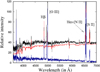 |
Fig. 1. Decomposition of the spectrum (SDSS J105621.57−005320.4) into the host galaxy and AGN contributions using SPCA. The black line shows observed data, the red line shows the host galaxy contribution obtained from SPCA, and the blue line shows the AGN contribution (host galaxy contribution subtracted from observed spectrum). |
2.2. Sample properties and selection effect
Histograms of the distribution of cosmological redshift and [O III]λ 5007 Å luminosity (L) for the sample of 577 AGNs are shown in Fig. 2 (grey bars). Using the described selection criteria we obtained a low-redshift AGN sample (z < 0.25) in which 95% of the objects have z < 0.125 and log(L[O III]5007 erg s−1) within the range [40.25−42].
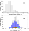 |
Fig. 2. (a) Histogram of the distribution of cosmological redshift for the total sample. (b) Histogram of the distribution of [O III]λ 5007 Å luminosity for the total sample (grey bars) and for different subsets (unblended subsample – blue bars, objects from unblended subsample with detected wing components in both Hα and [N II] lines – green bars, and the same but for [N II] and [S II] lines – red bars. |
We tested the influence of the selection criteria on the properties of the final sample, and find that the criterium of the line strength (criterium number 4: EWs of considered lines must be larger than 5 Å) has no significant influence on the redshift distribution of the sample, while deletion of this criterium leads to a larger number of objects with smaller luminosities of L[O III]5007. On the other hand, a decrease in the lower limit for S/N (criterium number 3) leads to a larger number of objects with slightly higher redshift and [O III] luminosity.
We conclude that criteria of the lower limit for S/N and lower limit for the line strength lead to the loss of spectra with slightly higher redshifts (z > 0.125) and a broader luminosity range. Although we lose the possibility to investigate the outflow in a greater diversity of objects, the criteria of high S/N and line strength are required for this investigation in order to enable the analysis of the asymmetries of the weak emission lines Hβ and [S II], which are diluted by the noise in spectra with lower S/N. Therefore, the chosen sample consists of the low-redshift AGNs with high-quality spectra and prominent emission lines, in which we can analyse the emission-line shapes very precisely.
2.3. The fitting procedure
We used a double-Gaussian or a single-Gaussian model for emission line decomposition, and applied a χ2 minimalisation routine to obtain the best-fit parameters, which is similar to the procedure followed for Type 1 AGNs in Popović et al. (2004) and Kovačević et al. (2010). The double-Gaussian model includes one Gaussian that fits the core of the line (core component) and another that fits the wings (wing component), which is often used to describe the narrow emission line shapes (see e.g., Mullaney et al. 2013; Woo et al. 2016; Sexton et al. 2021).
2.3.1. Decomposition of the [O III], Hβ, and [S II] lines
As the [O III], Hβ, and [S II] lines do not overlap with other lines in the spectra, they were fitted completely independently for the whole sample using a double-Gaussian (wing+core) model, where wing and core Gaussian components of each line have the free parameters of width, shift, and intensity. The only parameter constraint for these lines is done within doublets. The [O III] doublet is fitted in such a way that both doublet lines ([O III]λ 5007 Å and [O III]λ 4959 Å) have the same width and shift of the core (and wing) Gaussian, and the intensity ratio of doublet lines is fixed to be 2.99 (see Dimitrijević et al. 2007). The core and wing components of the [S II]λλ 6717, 6731 Å doublet are fitted with same widths and shifts for both doublet lines as well, but their intensity ratio is not fixed. In 16 objects, after removing the host galaxy contribution, we observed the weak broad Hβ originating from the broad line region (BLR), which is fitted with one broad Gaussian.
We find that in some spectra, the wing components of [O III], [S II], and Hβ have widths comparable to those of the core components, and their contribution to the line shape is very poor. Therefore, we adopted two criteria in order to avoid fake wing components: (i) a wing component amplitude-to-noise ratio (Aw/N) to be higher than 3 (wing components with Aw/N < 3 were neglected); and (ii) for the wing components that satisfy the first criterium, we applied the extra-sum-of-squares F-test (Lupton 1993) in order to check the justification of their implementation in the model, similarly to in Sexton et al. (2021). This test compares the improvement of the sum-of-squares using the more complicated model versus the loss of degrees of freedom in a simpler model. The test is done for wing components of each line separately, and wing components are adopted if the P-value < 0.05, for a null hypothesis that there is no significant improvement of the fit when applying the model that includes more parameters compared to the fit with the model with a smaller number of parameters. The wing components for which P-value is larger than 0.05 were neglected because one cannot be sure of their presence. In cases where wing components were neglected, the lines were fitted with a single-Gaussian model.
We find that the adopted double-Gaussian and single-Gaussian models accurately describe the line shapes of the majority of the [O III], Hβ, and [S II] lines. However, in ∼2% of objects from the sample, we noticed the complex shapes of the [O III] lines, and in some cases Hβ lines as well. We excluded the 12 most extreme cases from the correlation analysis, for which we found by visual inspection that their complex line shapes could not be fitted with the adopted models. These objects were analysed separately in Appendix A.
2.3.2. The division to the ‘unblended’ and ‘blended’ subsamples
To correctly decompose the [N II]+Hα wavelength band, we adopted the following procedure: we divided the whole sample into two subsamples – one that consists of spectra where [N II] and Hα lines are unblended, i.e. do not overlap with each other (hereafter ‘unblended’ subsample), and another where the [N II]+Hα wavelength band is blended (hereafter ‘blended’ subsample). The blended [N II]+Hα wavelength band could indeed be (a) the sum of the broaden wings of the [N II]+Hα lines which form a pseudo-broad component, (b) a true Hα BLR component, or, in the most complex cases, (c) both of these combined.
To form the unblended subsample, we single out all spectra from the total sample in which the emission line flux at ∼6575 Å (minimum between Hα and [N II] 6583 Å line) is smaller than 5% of the [N II] 6583 Å line intensity. In this way, we obtained 346 spectra in which Hα and [N II] 6583 Å lines do not overlap or overlap very slightly, i.e. flux at ∼6575 Å (Flux6575) is close to the continuum level. We find that in 80% of the objects from this subsample, the Flux6575 is at the level of the noise (Flux6575/N < 3). The rest of the spectra (219 objects, after excluding 12 objects with the complex [O III] shape) belong to the blended subsample. Following this separation criterium, the unblended spectra make up ∼60% and blended ∼40% of the total sample. Examples of the [N II]+Hα wavelength band in spectra from both subsamples are given in Fig. 3.
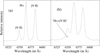 |
Fig. 3. [N II]+Hα wavelength band in spectra which belong to the (a) unblended and (b) blended subsamples (SDSS J100551.19+125740.6 and SDSS J112408.63−010927.9, respectively). |
We first performed the decomposition of the Hα and [N II] lines for the unblended subsample, and then used the empirical relationships found in the unblended subsample to establish the decomposition procedure for blended subsample (see Sect. 3.4). The Hα and [N II] lines in the unblended subsample are fitted independently with a double-Gaussian model, without any parameter constraints for the core or wing components. Therefore, they are fitted in the same way as the [O III], Hβ, and [S II] lines in the total sample. The decomposition of the [N II]λλ 6548, 6583 Å doublet lines was done in a similar way to the decomposition of the [O III] doublet: both doublet lines ([N II]λ6548 Å and [N II]λ 6583 Å) have the same width and shift of the core (and wing) Gaussian, and the ratio of doublet lines is 3.05 (see Osterbrock & Ferland 2006). As for the [O III], [S II], and Hβ lines, the wing components of the Hα and [N II] lines in the unblended subsample were adopted only if they satisfy the criteria of Aw/N > 3 and F-test (P-value < 0.05). In the cases where wing components did not satisfy one of these criteria, the Hα and [N II] were fitted with a single-Gaussian model.
An example of the fit of all the considered lines for a spectrum from the unblended subsample is shown in Fig. 4, while the decomposition of the blended subsample is presented in Sect. 3.4.
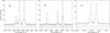 |
Fig. 4. Example of fit decomposition for object SDSS J125025.82+001954.9 from the unblended subsample: (a) Hα and [N II], (b) Hβ and [O III], and (c) [S II]. The core components are denoted with a dotted line and the wing components with a solid line. |
2.4. Measuring the spectral parameters
In this investigation, we analysed the gas kinematics using the velocity shift and width (dispersion) of the separated core and wing Gaussian components obtained from the best fit. The fitting procedure was done after systemic correction of spectra for cosmological redshift (determined using galaxy eigenspectra; see Bolton et al. 2012), and the velocity shifts of components were measured relative to the transition wavelength in rest-frame spectra.
The uncertainties on the line fitting parameters were estimated for each line in each spectrum by applying a Monte Carlo method. We used the measured values from the emission-line fits to construct the model, and then made 100 mock spectra for each source by adding random noise to the model spectra. The random noise was limited to not exceed the measured 3σ noise for each object. After we obtained the fitting parameters of the mock spectra, we took the 1σ dispersion of the parameters as the fit uncertainty. The lines with small intensities, [S II] and Hβ, are found to have larger uncertainties than the other considered lines in the spectra. The mean shift and width uncertainties for wing components of [S II] are 46 km s−1 and 37 km s−1, those for Hβ are 41 km s−1 and 30 km s−1, and for [N II], Hα, and [O III] these values are in the range of 9−13 km s−1. The mean shift and width uncertainties for the core components of all considered lines, as well as for single-Gaussian lines, are in the range 1−8 km s−1.
The widths of the wing Gaussian components are corrected for instrumental SDSS width following the formula:  , where σobs is the Gaussian width measured from the spectrum, σinst is the instrumental SDSS width, and σcor is the corrected dispersion used in the analysis. SDSS provides the σinst measured for different lines for each object, which we used for data correction. In this sample, the instrumental widths are within the interval 48−83 km s−1.
The stellar velocity dispersions (σ*) are obtained from SDSS (Thomas et al. 2013). The measurements are based on adaptations of the publicly available codes GANDALF v1.5 (Sarzi et al. 2006) and pPXF (Cappellari & Emsellem 2004), which are used to fit stellar populations and evaluate the stellar kinematics. Although this procedure is primary applied for the BOSS massive galaxies (z > 0.15, see Dawson et al. 2013), Thomas et al. (2013) demonstrated that σ* estimates using this algorithm are reliable for a general galaxy sample. The σ* of SDSS spectra were extracted with a 3″ aperture and they may be affected by rotational broadening and the inclination effect. All σ* below the SDSS instrumental resolution of 70 km s−1 were excluded from the analysis.
3. Results
3.1. The line profiles: gravitational vs. non-gravitational contribution
Although the double Gaussian model (core+wing component) is frequently applied in narrow emission line decomposition, there is still concern among authors over the physical meaning of that decomposition (see e.g., Zhang et al. 2011; Davies & Förster Schreiber 2020b). Interesting questions refer to whether or not wing and core components dominantly represent emission from different emission regions; and whether or not it is justified to analyse them separately, and if so, is this is true for all narrow emission lines?
Previous investigations of the influence of gravitation on the narrow emission line profiles mostly compared the total line profile width with σ* (Greene & Ho 2005a; Woo et al. 2016, 2017; Kang et al. 2017, etc.), where σ* is assumed to be a good indicator of the gravitational motion. The widths of the wing and core components were rarely used separately in a correlation analysis with σ*, except in a few studies of Type 1 AGNs, and only for the [O III] lines (Xiao et al. 2011; Sexton et al. 2021).
Here we investigated the influence of gravitational motion on the widths of the separated wing and core components of different lines. We tried to verify whether or not these components dominantly originate in kinematically different gas in our sample, and whether or not there is a difference between the considered lines related to the influence of gravity or outflows. We plotted the widths of the core and wing components versus σ* for lines decomposed with the double-Gaussian model. Additionally, in the same graphs we added the widths of single-Gaussian lines versus σ*. Figure 5 shows these plots for the [O III], [S II], and Hβ lines for the total sample, and Fig. 6 shows these plots for Hα and [N II] lines for the unblended subsample, where these lines are fitted independently, without fitting constraints.
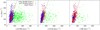 |
Fig. 5. Correlations between σ* and the widths of single-Gaussian lines (red dots), and the wing and core components of the double-Gaussian lines (green and blue dots) for [O III], [S II], and Hβ lines (total sample). The one-to-one relation is denoted with the solid line. |
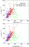 |
Fig. 6. Same as in Fig. 5, but for Hα and [N II] lines. The correlations are shown for the ‘unblended’ subsample, where Hα and [N II] lines are fitted independently. The one-to-one relation is denoted with a solid line. |
We find that the widths of the wing components of the [O III], [S II], Hα, [N II], and Hβ lines (denoted with green dots in Figs. 5 and 6) show no correlation with σ*, which implies their non-gravitational origin in all these lines. On the other hand, the widths of the core components of the double-Gaussian lines (blue dots in Figs. 5 and 6) are in significant correlation with σ* for the [S II], Hα, and [N II] lines, which implies their dominantly gravitational origin. However, the widths of the [O III] core components are in weak correlation with σ*, while no correlation is found between the widths of the Hβ core components and σ*. The coefficients of correlations of different lines versus σ* are given in Table 1. The weak correlation of the [O III] core component width with σ* implies that in addition to a gravitational influence, the [O III] core components are probably affected by a non-gravitational influence in our sample, which is in accordance with previous results (Karouzos et al. 2016a; Woo et al. 2016; Sexton et al. 2021). Similarly, the lack of correlation between the width of the Hβ core components and σ* could be caused by a strong non-gravitational influence in the core component as well, but also it could be partly caused by the small number of detected double-Gaussian Hβ lines in the sample. Contrary to the core components, significant correlations are found for the widths of the single-Gaussian [O III] and Hβ lines versus σ*. Generally, we find that the widths of the single-Gaussian emission lines (red dots in Figs. 5 and 6) are in stronger correlation with σ*, comparing the core components of the same kinds of lines. We note that, for σ* > 170 km s−1, stellar velocity dispersions become slightly larger than widths of the core components and the single-Gaussian lines. This could be caused by overestimation of the stellar velocity dispersion obtained with the SDSS aperture, which is due to the contribution of the rotational broadening and inclination effect, as found in Eun et al. (2017).
Correlations between the stellar velocity dispersion (σ*) and velocity dispersions of the core components of double-Gaussian lines and single-Gaussian lines.
In summary, our analysis implies that the non-gravitational (outflow) contribution is dominantly present in wing components of all the lines analysed here, while non-gravitational effects also partly contribute in the [O III] and Hβ core components. As extraction of the non-gravitational contribution from the [O III] and Hβ core components is a complicated task, we focus on the wing components of the considered lines (green dots in Figs. 5 and 6) in order to investigate the pure non-gravitational kinematics of the different lines.
3.2. Presence of the wing components in line profiles
We find that the number of detected wing components is significantly different among the considered emission lines in our sample. The wing components most frequently occur in the [O III] line profiles. Moreover, in the large number of spectra, wing components are seen only in the [O III] lines, but not in the other lines (Hβ, Hα, [N II], and [S II]). In these cases, [O III] wing components are weak and just slightly broader than the [O III] core component. Opposing cases, where wing components are seen in some other lines but not in [O III], are rare.
In the total sample of 577 objects, the wing components are detected in the [O III] profile for 426 objects, in the [S II] profiles for 150 objects, and in the Hβ lines in only 52 objects. A similar trend is present if we consider only the unblended subsample (346 objects), where Hα and [N II] are also fitted without parameter constraints. In this subsample, the wing components are detected in the [O III] profiles for 229 objects, in the Hα profiles for 70 objects, in the [N II] profiles for 85 objects, in the [S II] profiles for 35 objects, and in the Hβ profiles for only 8 objects. To understand the results of the decomposition, it is very important to understand whether the lack of wing components in the single-Gaussian lines is caused by a physical phenomenon or is due to selection effects of the criteria (Aw/N > 3 and F-test; see Sect. 2.3.1) used to include the wing component in the model of decomposition.
The frequent presence of the [O III] wing components in the total sample could be partly explained by the significantly stronger intensity of the [O III] lines compared to the other analysed emission lines in the spectra, especially [S II] and Hβ, which have generally small intensities in this sample, and similar fitting uncertainty due to noise. Although the spectra are chosen to have high S/N, it is still possible that the wing components of the [S II] and Hβ lines are diluted by the noise, i.e. reduced by the requested criterium of Aw/N > 3 for the wing components. Additionally, the weak Hβ wing components could be lost in the process of host galaxy subtraction. Namely, host galaxy spectra may have absorption in the Hβ line, and in these cases, it is very difficult to correctly reproduce the wing component in the Hβ emission line profile. In 52 objects, where Hβ wing components are detected, the host galaxy spectra have no absorption in Hβ, or this absorption is very small. Another concern is possibility that the wing components that are not shifted compared to the core components and which are not significantly broader than them could be reduced by the F-test. Namely, if the line profiles could be fitted very well with a single-Gaussian model, then including the additional Gaussian component is not statistically justified. We find that the average widths of the single-Gaussian lines are slightly broader than the average widths of the core components of the double-Gaussian lines. Only in the case of [O III] are these average values similar. The histogram of the distribution of the single-Gaussian widths and core component widths for [S II] lines is given in Fig. 7. In ∼10% of the single-Gaussian [S II] lines, the width exceeds the range of widths of the core component. A similar trend is observed for the Hβ line. These objects are possible candidates for hidden wing components which remain undetected because of our conservative criteria for wing-component detection. We can conclude that, in addition to physical effects, the number of detected wing components for different lines could also be affected by the noise for the weak lines, the small shift of the wing components relative the line core, and host galaxy absorption, which is especially important for the Hβ lines.
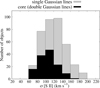 |
Fig. 7. Histogram of the width distribution of the single-Gaussian [S II] lines and the core components of the double-Gaussian [S II] lines. |
3.3. Wing component correlations in the unblended subsample
In this section, we use the unblended subsample, in which [N II] and Hα lines are fitted independently, in order to search for relationships between the wing components of these lines, which can be used to reduce the fitting parameters in the case of the complex and blended [N II]+Hα wavelength band. The unblended subsample contains 346 spectra, of which 229 AGN spectra have at least one wing component present.
The most significant correlations are found between the shifts of the [N II], Hα, and [S II] wing components (see Fig. 8). The Pearson coefficient of the correlation between shifts of the [N II] and Hα wings is r = 0.81, P = 9.3E−15, that between [N II] and [S II] wings is r = 0.79, P = 5.5E−8, and that between Hα and [S II] wings is r = 0.80, P = 2.3E−7, where the P-value is the probability that there is no correlation. The number of objects included in these correlations depends on the number of detected wing components in both lines. For [N II] and Hα, this number is 57, for [N II] and [S II] it is 32, and for Hα and [S II] it is 30 objects (∼90% of the objects are common to the latter two subsamples). To investigate the relationship between the data, we applied the method of least squares for simple linear regression model. In Fig. 8 we gave the obtained parameters of the fit (slope and intercept) with parameter standard errors and we shade the 95% confidence interval region. The linear fit between each pair of these three lines gives a one-to-one relationship, within the error bars.
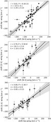 |
Fig. 8. Correlations between the shifts of the [N II], [S II], and Hα wing components in the unblended subsample (r – coefficient of correlation, and appropriate P-value are given). The data are fitted with a linear function Y = k ⋅ X + n (solid line), where k is the slope and n the intercept of the best linear fit. The one-to-one relation is denoted with a dashed line. The shaded region corresponds to the 95% confidence interval. |
As the requirement for making the unblended subsample was so that [N II] and Hα wing components do not overlap at 6575 Å (or overlap very slightly), this subsample is strongly biased by spectra with wing components with small widths. Therefore, the lack a width–width correlation between wing components is expected because of the narrow range of the wing component widths. However, despite a limited sample, a significant correlation is found between the widths of the [N II] and Hα wing components (r = 0.68, P = 4.2E−9), which is slightly weaker than that found between their shifts. The linear fit also gives an approximately one-to-one relationship (see Fig. 9). We notice that, in the spectra where both [O III] and Hα wing components are present, the widths of the [O III] wing components are larger than those of Hα components in ∼65% of cases. In these spectra, the differences between the widths of the [O III] and Hα wing components go up to 500 km s−1. In ∼35% of cases, the widths of the Hα wing components exceed the widths of the [O III] wing components, and their differences go up to 150 km s−1. A similar trend is observed between the [O III] and [N II] wing component widths. These findings are in accordance with previous studies (Karouzos et al. 2016a; Bae et al. 2017; Kang et al. 2017; Kang & Woo 2018), which found that the outflow contribution is generally stronger in [O III] lines compared to Hα lines. Therefore, we do not expect the widths of the Hα or [N II] wing components to significantly exceed the width of the [O III] wing components in the rest of the our sample.
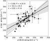 |
Fig. 9. Correlations between the widths of the [N II] and Hα wing components in the unblended subsample. Notation is the same as in Fig. 8. |
We find that the unblended subsample, as well as small subsets of the unblended subsample in which we found the above mentioned correlations, show a similar distribution of L[O III] to that shown by the total sample (see Fig. 2b). We assume that the correlations found are maintained throughout the rest of the sample, which has broader wing components included. Therefore, we adopted the strongest correlations found in this subsample for fitting constraints in the rest of the spectra with blended [N II]+Hα.
3.4. Procedure for decomposition of blended [N II]+Hα
The most complicated part of the fitting procedure of the Type 1.8-2 AGN spectra is the spectral decomposition of the blended [N II]+Hα wavelength band, because in some spectra, these lines have very broaden wings that overlap each other. An additional complication is the possible presence of a broad Hα component (see Woo et al. 2014; Oh et al. 2015; Eun et al. 2017), which arises in the BLR and in some cases barely differs from the sum of the three broaden wing components. As the [N II]+Hα wavelength band is blended in ∼40% of our sample, unraveling the complex kinematical properties in these objects is crucial for a comprehensive analysis of the outflow contribution in the Hα and [N II] lines.
In previous studies that dealt with the complex [N II]+Hα wavelength band, reduction of the fitting parameters was done using assumptions, and not by using systematically and empirically proven relationships between fitting parameters on a large sample. The most frequently used assumptions were the same widths and shifts of the [S II] and [N II] Gaussian components, or scaling the [S II] line shape to the [N II] and Hα lines (see e.g. Filippenko & Sargent 1988; Ho et al. 1997; Popović et al. 2004; Greene & Ho 2005b; Trippe et al. 2010; Karouzos et al. 2016a; Luo et al. 2019, etc.). Here we use the outcomes of our analysis of the kinematical properties of the unblended subsample presented in the previous section to design a procedure for the decomposition of the [N II]+Hα wavelength band in the blended subsample. The presented fitting procedure can be applied only if the outflow emission in the [O III] lines can be approximated well with a single Gaussian wing component. In the cases where [O III] lines have peculiar profiles with a complex outflow contribution, a more complex analysis is needed to decompose the [N II]+Hα region (see Appendix A.1).
We note that spectra with blended [N II]+Hα can be divided into two groups:
(a) objects where the presence of the Hα BLR in the blended [N II]+Hα wavelength band is uncertain. In these objects, there is no flux that extends significantly out of the [N II] doublet. Therefore, each of the three scenarios are possible: the blended [N II]+Hα can be composed of one broad Hα component, the sum of three broaden wing components of [N II] and Hα, or in the most complicated cases, both combined, that is, a weak Hα BLR nested under [N II]+Hα wing components;
(b) objects where the presence of the Hα BLR is certain. In these objects, the broad wings of Hα BLR component extend distinctly from both sides of the [N II] doublet, and therefore its presence is clear, even by simple visual inspection.
We established the following fitting procedure for objects which belong to group (a).
1. Check if Hβ BLR is present. In the case that Hβ BLR is present in the spectrum, the Hα BLR component should be included as well. Hα and [N II] wing components should only be additionally included (with reduced fitting parameters as defined below) if obvious asymmetry is present in narrow lines.
2. If [O III] lines have no wing components detected, or if they have weak and narrow wing components (their width is not much broader than the width of the [O III] core), Hα BLR should be included in the model. In these spectra, Hα BLR dominantly fits blended [N II]+Hα, and Hα and [N II] wing components should be included only if needed to fit the shape of the narrow lines.
3. If the [O III] lines have strong and broad wing components, then we expect that the sum of the three wing components of [N II] and Hα dominates in the blended region. Therefore, the blended [N II]+Hα should be fitted with the three wing components using the following fitting constraints. (i) shift Hα wing = shift [N II] wing = shift [S II] wing. (ii) width Hα wing = width [N II] wing.
The [S II] lines should be fitted first, and the obtained value of the wing component shift should be used to fix the shift of Hα and [N II] wing components. If there are no [S II] wing components detected, then the shift of Hα and [N II] wing components is one free parameter. Additionally, it is recommended to keep Hα and [N II] wing component widths to not exceed the width of the [O III] wing component by much (see Sect. 3.3). In this way, we avoid the possibility that three unreal, extremely broaden wing components obscure the potential presence of the one true broad Hα component. If the fit with three wing components, limited with the mentioned fitting constraints, cannot accurately describe the shape of the complex [N II]+Hα wavelength band, then the Hα BLR component should be included.
The objects from group (b), where the Hα BLR component distinctly extends from both sides of the [N II] doublet, should be fitted with one broad component, and the wing components should only be included if narrow lines show asymmetry. In the case where they are needed, the wing components should be fitted with parameter constraints as defined above, for group (a). Generally, Hα BLR component should only be adopted if it satisfies the criterium of amplitude-to-noise ratio larger than 3. Otherwise, it should be neglected, because it is unreliable.
By applying a very careful spectral decomposition of objects from group (a), we find only nine nested Hα BLR components with full width at half maximum (FWHM) within the range of 2050−3000 km s−1, while the rest of the objects from group (a) are fitted with sum of the three wing components. Examples of spectral decomposition of the objects from group (a), with and without a nested Hα BLR component, are shown in Fig. 10. We find 46 objects from the blended subsample that clearly show a very broad Hα BLR component (group (b)). Their FWHMs are in the range of 3040−10 600 km s−1, which makes them much broader than the wavelength range of the [N II] doublet. An example fit of the complex spectra from group (b) is shown in Fig. 11.
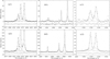 |
Fig. 10. Example of decomposition of objects from the blended subsample (group a): SDSS J010946.70+134411.9 (a1, b1, c1) and SDSS J111848.44+280738.3 (a2, b2, c2). The blended Hα+[N II] is decomposed as: nested Hα BLR and three weak wing components in panel a1 and with three strong wing components in panel a2. The decomposition of the [O III] and Hβ is shown in panel b1 and b2, and decomposition of the [S II] lines is shown in panels c1 and c2. The core and wing components are denoted with the dotted and solid line, respectively. |
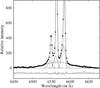 |
Fig. 11. Example of the complex decomposition of the [N II]+Hα wavelength band for object (SDSS J032525.36−060837.8) with a distinctly extended Hα BLR component (group b). The [N II]+Hα is decomposed into the [N II] and Hα core and wing components, and one Hα BLR component. The core components are denoted with the dotted line, and wing components and Hα BLR are shown with a solid line. |
In summary, we find that 55 objects belong to the Type 1.9/1.8 AGNs, which make up ∼25% of the spectra with blended [N II]+Hα in our sample. The rest of objects are Type 2 AGNs with strong wing components whose sum could be misinterpreted as broad Hα, as noticed in other studies (Woo et al. 2014; Eun et al. 2017).
3.5. Correlations between the wing components in the total sample
After decomposing the [N II]+Hα in the blended subsample, we merged the two subsamples, unblended and blended, in order to look for correlations between the wing components in the total sample. As we reduced the fitting parameters in the blended subsample, as described in Sect. 3.4, we only analysed the relations between the independent line parameters for the total sample. These are, width and shift of Hα wing components, width of [S II], and widths and shifts of the Hβ and [O III] wing components, which are fitted independently in the total sample.
We find that the wing component shifts of all analysed lines are in significant correlation, as are their widths, with the exception of the width of Hβ wings which do not correlate with the widths of the other lines. The correlations between the mentioned line parameters are given in Table 2.
Correlations between the widths and shifts of the wing components (w) of different lines in the total sample (unblended + blended).
The coefficient of correlation between the wing component shifts of the [O III] and Hα is r = 0.64, P < 1E−17 and this relationship is shown in Fig. 12a, where blended and unblended subsamples are denoted with different symbols. The significant correlations between the shift of the Hβ wing components and the shifts of the [O III] and Hα wing components are shown in Fig. 13.
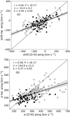 |
Fig. 12. Correlation between the shifts (top) and widths (bottom) of the [O III] and Hα wing components for the total sample. The unblended subsample is denoted with full circles and the blended subsample with open circles. The Pearson coefficient of correlation (r), P-value, slope (k), and intercept (n) of the best linear fit (solid line) are given. The dashed line represents the one-to-one relation and the shaded region corresponds to the 95% confidence interval. |
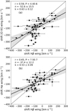 |
Fig. 13. Correlations between the shift of the Hβ wing components and the shifts of the [O III] (top) and Hα (bottom) wing components for the total sample. The notation is the same as in Fig. 8. |
The total sample has a larger range of wing component widths compared to the unblended subsample, and therefore we find significant correlations between the widths of the [O III], Hα, and [S II] wing components (r = 0.41 − 0.58, see Table 2), which cannot be seen in the subsample with a smaller range of the widths. The only exception, the Hβ wing components, have the weakest statistics (only 52 objects) and the least reliable fit compared to the other wing components, because of the low intensity of the Hβ lines and a possible influence of the host galaxy absorption on the Hβ wing component profiles. Also, the physical meaning of the decomposition into the core and wing components is unclear for the Hβ line, because Hβ core components show no correlation with σ* (see Sect. 3.1). The correlation between the widths of the [O III] and Hα wing components is shown in Fig. 12b. Although the data show significant dispersion, the correlation is significant with a correlation coefficient of r = 0.58, P < 1E−17.
It is especially interesting to analyse the slopes of the shift–shift and width–width correlations between the wing components of the different lines. In the case of the Hα and [N II] wing components in the unblended subsample, the relationships were approximately one-to-one, within uncertainties. However, in the case of the Hα and [O III] lines, the slopes are much shallower, even when we consider uncertainties on the linear fit. The slopes indicate generally larger widths and larger blueshifts of the [O III] wing components compared to Hα. The difference becomes more significant with increasing blueshift of the [O III] wing component (< − 200 km s−1) and width of the [O III] wing component (> 250 km s−1), which can be seen in Fig. 12.
3.6. Comparison between mean wing component profiles
The mean wing component profiles for different lines in the unblended subsample are shown in Fig. 14a. To make the mean profiles of the [O III], [N II], and Hα wing components, we used the spectra from the unblended subsample in which all these wing components are present (57 objects). The mean wing component profile of the [S II] is made using all the observed [S II] wing components in the unblended subsample (35 objects). The intensities of all profiles are scaled to one and shift is measured relative to the transition wavelength for each line. As can be seen in Fig. 14a, all mean profiles are slightly blueshifted relative to their reference wavelength. The Hα mean profile has the smallest blueshift (−36 km s−1), while the largest blueshift is present for the [O III] mean wing component profile (−90 km s−1). A significant difference can be seen in their widths. The mean profile of the [O III] wing component is broader than the other mean profiles. The [N II] and Hα have almost identical mean profiles, while the narrowest is the mean [S II] profile. The outflow signature in the [N II] and Hα profiles appears very similar.
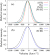 |
Fig. 14. Mean profiles of [O III], [N II], Hα, and [S II] wing components for the unblended subsample (a). The mean profiles of the [O III] and Hα wing components for the blended subsample (b). |
In the blended subsample, the mean wing component profiles of [O III] and Hα follow the same trend as that observed in the unblended subsample (see Fig. 14b)4. The profiles are made using 168 spectra with both wing components present. As expected, both profiles have larger widths and blueshifts compared to the mean profiles of the same lines from the unblended subsample. Similar to in the unblended subsample, the mean [O III] wing component is broader than Hα and shows a greater blueshift (−136 km s−1 for [O III] and −95 km s−1 for Hα). The objects with extreme [O III] wing component blueshifts (< − 200 km s−1), which deviate the most from the Hα wing component shifts, are present in ∼20% of blended spectra, and so they do not strongly contribute to the shift of the mean [O III] line profile. The broadest mean wing component profile is seen for the [O III] lines throughout the whole sample, which indicates that outflow kinematics is more strongly reflected in the [O III] profile than in all the other analysed lines.
4. Discussion
Here we discuss the results presented in Sect. 3 from various aspects. First, we discuss the problem of the estimation of the outflow contribution in emission line profile and the complex shapes of the outflow contribution. We then discuss the systemic influence of the outflow kinematics on the line profiles in the spectra, and the possible outflow emission-region stratification. Finally, we draw attention to the problem of the distinction of the sum of the three wing components from the true broad Hα in the blended [N II]+Hα wavelength band.
4.1. Extracting the outflow contribution in line profiles
The biconical outflow model predicts a large diversity of complex shapes for the outflow contribution, which depend on parameters such as outflow velocity, inclination, and amount of extinction material (see Bae & Woo 2016). In accordance with theoretical expectations, we observed complex shapes for the [O III] line profile (and in some cases also in Hβ) in 2% of our sample of SDSS spectra. Their detailed descriptions and comparison with the theoretically predicted shapes of the outflow contribution are given in Appendix A. In the remaining 98% of the sample, all considered lines can be well fitted with single- or double-Gaussian models (wing+core components). It is possible that some physical processes in the gas outflow may have a role in producing the Gaussian-like shape. Namely, the ‘Gaussianisation’ of the irregular and complex shape of the outflow contribution can be caused by microturbulence, which is found to be present in AGN-photoionised clouds (see Bottorff et al. 2000; Kraemer et al. 2007). It is possible that during the outflow propagation it comes to mixing of the hot wind fluid and cool gas clumps at the base of the wind (Westmoquette et al. 2007), which may cause the gas turbulence. Some of the possible mechanisms could be Rayleigh-Taylor instability, for a radiatively driven cloud, or Kelvin-Helmholtz instability, for a cloud entrained in a wind (Kraemer et al. 2007). These mechanisms may cause microturbulence, which may affect the shape of the outflow component, making it broader and more Gaussian-like.
Although the wing+core model accurately describes the line shapes in the majority of the sample, we find that the physical meaning of that decomposition is debatable for some lines. Following the results shown in Sect. 3.1 and additionally in Appendix B (where the influence of gravitation is analysed for Hα and [N II] using the total sample), we find that the core component can be considered as gravitationally dominant and the wing component as outflow dominant for the Hα, [N II], and [S II] lines, while it seems that the kinematics of the [O III] and Hβ lines is more complicated. It appears that the outflow contribution is significantly present in the core components of these latter lines as well, and this leads to a large dispersion in the σ core versus σ* relation.
Possible mixture of the outflow and gravitational contribution in the [O III] core components has been reported by several studies (Karouzos et al. 2016a; Woo et al. 2016; Sexton et al. 2021). Moreover, several investigations, which predominantly analysed the [O III] lines, claim that total emission line profiles (including the core component) could be dominated by outflow kinematics (Liu et al. 2013; Zakamska & Greene 2014; Jarvis et al. 2019; Davies et al. 2020a). Most of these studies performed spatially resolved observations, and so it is possible that outflow kinematics contributes more to the core components when observed in a smaller radius, closer to the outflow source. However, decomposition of the entire outflow contribution to the line profile is a very complicated task, and should be the goal of a future investigation.
4.2. Outflow signature in the AGN spectrum
In this study we performed a systematic analysis of the influence of the outflow kinematics on the diverse lines in AGN spectra by investigating the kinematical properties of the wing components. We find significant correlations between wing component shifts for all analysed lines ([O III], [N II], [S II], Hα and Hβ), and between their widths (with the exception of the Hβ wing components, which have the least reliable results). The significant correlations found between the widths and shifts of the wing components for diverse lines ([O III], [N II], [S II], Hα and Hβ) represent the signature of outflow kinematics in the AGN spectra.
Although correlations between wing component widths exist between almost all lines, the significance of these correlations is slightly lower than that found between their shifts, and there is larger dispersion in the data. Following the biconical model given in Bae & Woo (2016), one can expect that the velocity shift of the outflow component is probably dominantly affected by the dust extinction, and that the width of the outflow component is probably dominantly affected by bicone inclination and intrinsic outflow velocity. If we assume this model, then the very good correlations between wing component shifts can be explained by the same influence of the dust extinction on the observed outflow components of all emission lines in one object. On the other hand, the width of the wing component Gaussian is a more complex parameter, and interpretation of its physical meaning is more complicated. In Fig. A.1b, we show the complex [O III] shape with a double-peak outflow component, which probably represents a superposition of emission from both the approaching and the receding outflow cone in a system without dust extinction (following the model of Bae & Woo 2016). If one fits that outflow contribution with a single wing Gaussian, the obtained result would be the Gaussian wing component with a shift of ∼0 km s−1, whose width would actually represent double the value of the projected intrinsic outflow velocity (from the approaching and receding outflow cones).
Therefore, it is possible that more spectra from our sample with a Gaussian wing component shift of ∼0 km s−1 also have a double-peaked outflow component, but that it cannot be resolved because of the insufficient spectral resolution. In that case, their wing component width represents a double value of projected intrinsic outflow velocity, while the widths of the strongly shifted wing components reflect the projected intrinsic outflow velocity from only one side of the outflow cone. This may be the reason for the larger data dispersion and the weaker correlations between wing component widths.
4.2.1. Influence of the outflow on the profiles of different lines
Although the observed correlations indicate that outflow kinematics systemically affects the line profiles in AGN spectra, it seems that it reflects with different strength in profiles of different lines. The wing components occur in the [O III] lines twice as often as in the Hα and [N II] lines, and three times more than in the [S II] lines. The slopes of the width–width and shift–shift relationships between the [O III] and Hα wing components indicate a significantly stronger outflow signature in the [O III] lines, especially in the case of the very blueshifted or very broad [O III] wing components. On the other hand, both the widths and shifts of the wing components of the Hα and [N II] lines show a one-to-one relationship, reflecting similar outflow kinematics. The comparison of the mean wing component profiles of [O III], [N II], Hα, and [S II] lines revealed a small difference between their shifts, but a significant difference between their widths (Fig. 14). Considering only forbidden lines, it is interesting that the width of the mean wing component profiles decreases as the critical density and ionisation potential of the ions decrease. Therefore, the broadest is the [O III] mean wing component, followed by that of [N II], and the narrowest is that of [S II].
The relationships between the narrow line widths and atomic characteristics (ionisation potential and critical density) were investigated in several previous studies (see e.g. De Robertis & Osterbrock 1984, 1986; Ludwig et al. 2012), but for the total narrow line profiles which are affected by the rotational, core component. In this study, we observed this tendency separately for the wing components, which have a pure non-gravitational origin. As already mentioned, the biconical model (Bae & Woo 2016) predicts that outflow velocity strongly affects the width of the outflow component, which could explain the tendency observed in Fig. 14. If we suppose that electron density and outflow velocity are maximal closer to the central engine, and decrease along the outflow, one might expect the forbidden lines with higher critical density to arise in an outflow structure closer to the central engine, and to be affected by a stronger outflow velocity, while the lines with smaller critical densities could not be emitted in that region. In that case, the [O III] lines would dominantly originate in the outflow structure closer to the central engine, the [N II] would originate farther away, and [S II] lines would dominantly originate the furthest away, in the outflow region with the lowest density and outflow velocity. Taking into account the fact that the kinematical properties of the Hα and [N II] wing components are very similar, and that the mean wing component profiles have very similar shapes, it is possible that Hα and [N II] wing components are dominantly emitted in the same region in outflow structure. The analysis presented in Davies et al. (2020a) also implies stratification in the outflow emitting region: Hα and [O III] are emitted throughout most of the ionised cloud, while much of the [S II] line originates from mostly neutral gas, close behind the ionisation front where the electron density drops dramatically.
4.2.2. Comparison with previous studies
Using the large sample of approximately 37 000 SDSS low-redshift AGNs, Kang et al. (2017) compared the shifts and widths of the [O III] and Hα lines, calculated as the first and second moments of the total line profiles. As the total line profiles represent the sum of the gravitational and outflow contribution, their shapes reflect the physics of both emission regions. These authors found that the kinematical properties of the total Hα profiles correlate with those of [O III], but that the outflow contribution is weaker in Hα than in [O III]. These findings are in accordance with our results obtained by comparing only the wing (outflow) components of these lines.
However, the relationship between the wing component widths of Hα and [O III] performed in this work (see Fig. 12b) has a shallower slope compared to the relationship between the widths of the total line profiles given in Kang et al. (2017). Our results indicate that, as the widths of the [O III] wing component increase, they become significantly broader compared to the corresponding widths of the Hα wing components.
The different slopes of the relationships between Hα and [O III] widths found in these two studies could be due to several factors considering the sample properties and method of measuring the width, because we do not include in our measurement the width of the gravitational component. The large sample in Kang et al. (2017) contains objects with significantly lower S/N compared to the sample in this study. As they adopt the wing components only if their Aw/N ratio is larger than 3, it is possible that a significant number of wing components remain undetected in the noise, and so do not contribute to the total line profile. Also, Kang et al. (2017) conservatively excluded from the sample all objects identified as hidden Type 1 AGNs in Woo et al. (2014) and Eun et al. (2017), and additionally they excluded from the analysis all objects that are candidates to be hidden Type 1 AGNs, with Hα velocity dispersion > 700 km s−1. These kinds of objects are decomposed and are included in the analysis presented here.
4.3. Strong outflow emission or broad Hα?
Several studies have dealt with the problem of the hidden Hα BLR in spectra typically classified as Type 2 AGNs (Woo et al. 2014; Oh et al. 2015; Eun et al. 2017). One of the outcomes of the outflow kinematical analysis presented in this work is procedure for the Hα+[N II] decomposition which should help to establish whether or not the broad Hα is present in the blended Hα+[N II], i.e. whether objects are Type 2 or Type 1.9 AGNs. The problem of the identification of the true Hα BLR, as well as correct decomposition in the case of the Hα BLR+wings superposition, is especially significant for central black hole mass (MBH) estimation using the Hα BLR line parameters (see Greene & Ho 2005b). Misinterpretation of the sum of the three broaden wings of the Hα and [N II] lines as broad Hα emission may lead to incorrect estimation of the MBH using the false Hα BLR.
Our results imply that multiple lines should be analysed as one system in order to achieve physically correct spectral decomposition of the Hα+[N II] wavelength band. Misinterpretation of the Hα BLR/wing components can be avoided by analysing the [O III] outflow contribution, which can be used to favour one model over another for Hα+[N II] decomposition, as is described in Sect. 3.4. Thus, in borderline cases, if [O III] lines have very strong and broad wing components, the blended Hα+[N II] wavelength band certainly cannot be fitted as the only Hα BLR component with no wing components. Also, if [O III] wing components are weak and narrow, or completely missing, we cannot expect that the blended Hα+[N II] is the sum of the three strong and broad wing components of Hα and [N II]. Therefore, the shape of the [O III] outflow contribution (complex or Gaussian-like) and its strength (weak and narrow or strong and broad) have an important role in our understanding of the origin of the flux in blended Hα+[N II] in each spectrum. On the other hand, [S II] has two orders of magnitude lower critical density than [O III] lines, and so it will fade away in high-density outflow region, which still could be the region of efficient emission for [O III] (also for Hα and [N II]). Therefore, the total shape of the [S II] lines (core+wing) is not a suitable template for the total shape of Hα and [N II] narrow lines in the process of decomposition of blended Hα+[N II]. Namely, the presence of the wing components in [S II] lines implies the presence of the wing components in Hα and [N II] with the same shift (see Fig. 8) and generally larger widths, but their absence cannot be used as confirmation of the non-existence of the Hα or [N II] wing components (see Sect. 3.4).
In the case of the complex shapes of the [O III] outflow contribution (see Fig. A.1), decomposition of the blended Hα+[N II] is even more complicated, and becomes a real challenge. It is expected that the complex and peculiar shape of the outflow emission seen in [O III] could be seen in the shapes of the other lines in the spectra as well. However, it should be taken into account that Hβ and [S II] lines are weaker than [O III], Hα, and [N II] in the spectra of Type 2 AGNs, and therefore their complex outflow shapes can be diluted by noise, or reduced by the high density of the outflow region in the case of [S II].
To illustrate the decomposition of Hα+[N II] in objects with strong and complex outflow emission in [O III], we used the object SDSS J013706.95−090857.4, which is analysed in Appendix A, and shown in Fig. A.1a as an example of the complex outflow emission. We tried to decompose blended Hα+[N II] in this object by adopting the same shape of the outflow component as extracted from [O III] (see Fig. A.1a1) for outflow components of Hα and [N II] lines. The details of the fitting procedure of the Hα+[N II] using this complex outflow shape are given in Appendix A.1. The decomposition of the blended Hα+[N II] is shown in Fig. 15a. As can be seen, the sum of the three complex outflow components, with a shape as seen in the [O III] lines, fits the emission flux under Hα+[N II] very well. It should be pointed out that the flux of the blended Hα+[N II] in SDSS J013706.95−090857.4 distinctly extends blueward of the [N II] doublet, giving the impression upon visual inspection that it is obviously an Hα BLR component. Without considering the extremely strong outflow emission in [O III], it could be fitted with a single broad Gaussian with FWHM = 2600 km s−1 (see Fig. 15b), interpreted as a Hα BLR component, and potentially used for MBH estimation as was done for this object in several studies analysing large data samples (Greene & Ho 2007; Oh et al. 2015; Liu et al. 2019). A more detailed investigation is needed to interpret the real nature of the blended Hα+[N II] in this object.
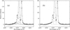 |
Fig. 15. Decomposition of the blended Hα+[N II] for object with a complex shape of the [O III] outflow emission (SDSS J013706.95−090857.4, see Fig. A.1a). The decomposition is done with (a) the sum of the three complex outflow components of the Hα and [N II] doublet, with the same shape as in [O III] lines (see Fig. A.1a1); and (b) with a single broad Gaussian with FWHM ∼ 2600 km s−1. The core components are denoted with a dashed line, and outflow components/broad Gaussian with a solid line. |
5. Conclusions
In this study, we used 577 spectra of Type 1.8-2 AGNs with high S/N obtained from SDSS in order to trace the outflow kinematics. We applied a very careful spectral decomposition of several emission lines (Hβ, [O III], Hα, [N II], and [S II]) using a single- and a double-Gaussian model (wing+core components), where wing components are taken to be a proxy of the outflow contribution. In order to investigate the outflow contribution in Hα and [N II] lines in the total sample, we focused on unravelling the complex kinematics of the blended [N II]+Hα, which is present in ∼40% of our sample. We used the outcomes of the analysis of the subsample with unblended Hα and [N II] lines in order to obtain fitting constraints and establish a procedure for decomposition of the blended [N II]+Hα.
We investigated the influence of the outflow kinematics on the line profiles by analysing the correlations between several kinematical parameters and by comparing the wing component mean profiles for different lines using the subsets in which wing components are present in the analysed lines. In this way, we investigated the systemic influence of the outflow kinematics on the different lines in the spectra, as well as the difference in the extent to which each line is affected by outflow kinematics. Summarising the main results, we can outline the following conclusions:
-
(i)
The outflow kinematics has a systemic influence on the considered emission lines in AGN spectra (Hβ, [O III], Hα, [N II], [S II]), which can be seen through strong correlations between their wing component shifts, as well as between their wing component widths. These correlations are found between each pair of lines, in subsets where wing components are detected in both compared lines. The only exception are the Hβ wing component widths (Hβ wing components are the least reliable and have the weakest statistics). Generally, the correlations between wing component shifts are slightly stronger compared to the correlations between wing component widths for all lines. It is possible that wing component shifts dominantly reflect the amount of extinction material, as predicted by the biconical model, while wing component width seems to be a more complex parameter, and to be affected with different projections of the outflow velocity, which probably cause the larger dispersion in the width–width correlations.
-
(ii)
The signature of the outflow kinematics differs for different lines. By comparing the line component dispersions with stellar velocity dispersion, we find that the wing components of all the considered emission lines have pure non-gravitational kinematics. The core components are consistent with gravitational kinematics for Hα, [N II], and [S II] lines, while in [O III] there is evidence for a contribution from non-gravitational kinematics. On the other hand, we find that all single Gaussian lines (with no wing component detected) represent gravitationally dominant kinematics. The comparison of the mean width of the wing components in subsets in which wing components are detected in all lines reveals that the [O III] wing components are generally broader than the wing components of the other analysed lines. The widths of the Hα and [N II] wing components are very similar, while the widths of the [S II] wing components are generally the narrowest. If we assume that outflow velocity strongly affects the width of the outflow component, as predicted by biconical model, then the difference in width may imply that these lines dominantly arise in different parts of an outflowing region.
-
(iii)
The blended Hα+[N II], which can be the sum of the three strong wing components, the true broad Hα, or both of these combined, can be successfully decomposed using the outcomes of the analysis of the subsample with unblended Hα and [N II] lines. The obtained parameter constraints prevent misinterpretation of the sum of the three wing components of Hα and [N II] as the Hα BLR or vice versa. Generally, in order to achieve a physically correct spectral decomposition of the blended Hα+[N II], multiple lines in the spectra should be analysed as one system, because their shapes systemically reflect the physical conditions in the outflow emission region. Particular care should be taken if extended and complex emission is observed in [O III]. In that case, the sum of the complex outflow emission of Hα and [N II] can mimic the broad Hα with FWHM up to ∼2600 km s−1, which makes spectral decomposition these objects very difficult.
-
(iv)
Although the biconical outflow model predicts a large diversity of complex shapes for the outflow contribution, we find the complex [O III] shapes only in ∼2% of the sample, while the rest of the sample can be well fitted with a single or a double-Gaussian model. It is possible that microturbulence, which could arise because of mixing of the hot wind fluid and cool gas during the outflow propagation, is responsible for making the complex outflow line shapes more ‘Gaussian-like’ in the majority of spectra.
The procedures for computations of galaxy properties given in Bolton et al. (2012) and Thomas et al. (2013) (primarily made for DR9) have been applied to all DR14 objects that the spectroscopic pipeline classifies as a galaxy. The measurements are available in SDSS Tables.
Acknowledgments
We thank anonymous referee for valuable comments and suggestions that helped us to significantly improve the paper. This work is supported by the Ministry of Education, Science and Technological Development of Serbia (451-03-9/2021-14/20016 and 451-03-68/2020-14/200002). Funding for the Sloan Digital Sky Survey IV has been provided by the Alfred P. Sloan Foundation, the US Department of Energy Office of Science, and the Participating Institutions. SDSS-IV acknowledges support and resources from the Center for High Performance Computing at the University of Utah. The SDSS website is www.sdss.org. SDSS-IV is managed by the Astrophysical Research Consortium for the Participating Institutions of the SDSS Collaboration including the Brazilian Participation Group, the Carnegie Institution for Science, Carnegie Mellon University, Center for Astrophysics, Harvard & Smithsonian, the Chilean Participation Group, the French Participation Group, Instituto de Astrofísica de Canarias, The Johns Hopkins University, Kavli Institute for the Physics and Mathematics of the Universe (IPMU)/University of Tokyo, the Korean Participation Group, Lawrence Berkeley National Laboratory, Leibniz Institut für Astrophysik Potsdam (AIP), Max-Planck-Institut für Astronomie (MPIA Heidelberg), Max-Planck-Institut für Astrophysik (MPA Garching), Max-Planck-Institut für Extraterrestrische Physik (MPE), National Astronomical Observatories of China, New Mexico State University, New York University, University of Notre Dame, Observatário Nacional/MCTI, The Ohio State University, Pennsylvania State University, Shanghai Astronomical Observatory, United Kingdom Participation Group, Universidad Nacional Autónoma de México, University of Arizona, University of Colorado Boulder, University of Oxford, University of Portsmouth, University of Utah, University of Virginia, University of Washington, University of Wisconsin, Vanderbilt University, and Yale University.
References
- Abolfathi, B., Aguado, D. S., Aguilar, G., et al. 2018, ApJS, 235, 42 [NASA ADS] [CrossRef] [Google Scholar]
- Bae, H.-J., & Woo, J.-H. 2016, ApJ, 828, 97 [Google Scholar]
- Bae, H.-J., Woo, J.-H., Karouzos, M., et al. 2017, ApJ, 837, 91 [NASA ADS] [CrossRef] [Google Scholar]
- Baldwin, J. A., Phillips, M. M., & Terlevich, R. 1981, PASP, 93, 5 [Google Scholar]
- Berton, M., & Järvelä, E. 2021, Universe, 7, 188 [NASA ADS] [CrossRef] [Google Scholar]
- Blanton, M. R., Bershady, M. A., Abolfathi, B., et al. 2017, AJ, 154, 26 [Google Scholar]
- Bolton, A. S., Schlegel, D. J., Aubourg, É., et al. 2012, AJ, 144, 144 [NASA ADS] [CrossRef] [Google Scholar]
- Bottorff, M., Ferland, G., Baldwin, J., & Korista, K. 2000, ApJ, 542, 644 [NASA ADS] [CrossRef] [Google Scholar]
- Cappellari, M., & Emsellem, E. 2004, PASP, 116, 138 [Google Scholar]
- Costa, T., Pakmor, R., & Springel, V. 2000, MNRAS, 497, 5229 [Google Scholar]
- Crenshaw, D. M., Schmitt, H. R., Kraemer, S. B., Mushotzky, R. F., & Dunn, J. P. 2010, ApJ, 708, 419 [Google Scholar]
- Davies, R., Baron, D., Shimizu, T., et al. 2020a, MNRAS, 498, 4150 [Google Scholar]
- Davies, R., Förster Schreiber, N. M., et al. 2020b, ApJ, 894, 28 [NASA ADS] [CrossRef] [Google Scholar]
- Dawson, K. S., Schlegel, D. J., Ahn, C. P., et al. 2013, AJ, 145, 10 [Google Scholar]
- De Robertis, M. M., & Osterbrock, D. E. 1984, ApJ, 286, 171 [NASA ADS] [CrossRef] [Google Scholar]
- De Robertis, M. M., & Osterbrock, D. E. 1986, ApJ, 301, 727 [NASA ADS] [CrossRef] [Google Scholar]
- Di Matteo, T., Springel, V., & Hernquist, L. 2005, Nature, 433, 604 [NASA ADS] [CrossRef] [Google Scholar]
- Dimitrijević, M. S., Popović, L. Č., Kovačević, J., Dačić, M., & Ilić, D. 2007, MNRAS, 374, 1181 [CrossRef] [Google Scholar]
- Eun, D., Woo, J.-H., & Bae, H.-J. 2017, ApJ, 842, 5 [NASA ADS] [CrossRef] [Google Scholar]
- Everett, J. E. 2005, ApJ, 631, 689 [NASA ADS] [CrossRef] [Google Scholar]
- Fabian, A. C. 2012, ARA&A, 50, 455 [Google Scholar]
- Filippenko, A. V., & Sargent, W. L. W. 1988, ApJ, 324, 134 [NASA ADS] [CrossRef] [Google Scholar]
- Greene, J. E., & Ho, L. C. 2005a, ApJ, 627, 721 [NASA ADS] [CrossRef] [Google Scholar]
- Greene, J. E., & Ho, L. C. 2005b, ApJ, 630, 122 [NASA ADS] [CrossRef] [Google Scholar]
- Greene, J. E., & Ho, L. C. 2007, ApJ, 667, 131 [NASA ADS] [CrossRef] [Google Scholar]
- Harrison, C. M., Alexander, D. M., Mullaney, J. R., & Swinbank, A. M. 2014, MNRAS, 441, 3306 [Google Scholar]
- Harrison, C. M., Costa, T., Tadhunter, C. N., et al. 2018, Nat. Astron., 2, 198 [Google Scholar]
- Ho, L. C., Filippenko, A. V., Sargent, W. L. W., & Peng, C. Y. 1997, ApJS, 112, 391 [NASA ADS] [CrossRef] [Google Scholar]
- Howarth, I. D. 1983, MNRAS, 203, 301 [NASA ADS] [CrossRef] [Google Scholar]
- Ishibashi, W., & Fabian, A. C. 2015, MNRAS, 451, 93 [NASA ADS] [CrossRef] [Google Scholar]
- Jarvis, M. E., Harrison, C. M., Thomson, A. P., et al. 2019, MNRAS, 485, 2710 [Google Scholar]
- Jarvis, M. E., Harrison, C. M., Mainieri, V., et al. 2021, MNRAS, 503, 1780 [NASA ADS] [CrossRef] [Google Scholar]
- Kang, D., & Woo, J.-H. 2018, ApJ, 864, 124 [NASA ADS] [CrossRef] [Google Scholar]
- Kang, D., Woo, J.-H., & Bae, H.-J. 2017, ApJ, 845, 131 [NASA ADS] [CrossRef] [Google Scholar]
- Karouzos, M., Woo, J.-W., & Bae, H.-J. 2016a, ApJ, 819, 148 [NASA ADS] [CrossRef] [Google Scholar]
- Karouzos, M., Woo, J.-W., & Bae, H.-J. 2016b, ApJ, 833, 171 [NASA ADS] [CrossRef] [Google Scholar]
- Komossa, S., Xu, D., & Wagner, A. Y. 2018, MNRAS, 477, 5115 [CrossRef] [Google Scholar]
- Kovačević, J., Popović, L. Č., & Dimitrijević, M. 2010, ApJS, 189, 15 [CrossRef] [Google Scholar]
- Kraemer, S. B., Bottorff, M. C., & Crenshaw, D. M. 2007, ApJ, 668, 730 [CrossRef] [Google Scholar]
- Kuraszkiewicz, J. K., Green, P. J., Forster, K., et al. 2002, ApJS, 143, 257 [NASA ADS] [CrossRef] [Google Scholar]
- Liu, G., Zakamska, N. L., Greene, J. E., Nesvadba, N. P. H., & Liu, X. 2013, MNRAS, 436, 2576 [NASA ADS] [CrossRef] [Google Scholar]
- Liu, H.-Y., Liu, W.-J., Dong, X.-B., et al. 2019, ApJS, 243, 21 [NASA ADS] [CrossRef] [Google Scholar]
- Ludwig, R. R., Greene, J. E., Barth, A. J., & Ho, L. C. 2012, ApJ, 756, 51 [NASA ADS] [CrossRef] [Google Scholar]
- Luo, R., Woo, J.-H., Shin, J., et al. 2019, ApJ, 874, 99 [NASA ADS] [CrossRef] [Google Scholar]
- Lupton, R. H. 1993, Statistics in Theory and Practice (Princeton: Princeton University Press) [CrossRef] [Google Scholar]
- Molyneux, S. J., Harrison, C. M., & Jarvis, M. E. 2019, A&A, 631, A132 [NASA ADS] [CrossRef] [EDP Sciences] [Google Scholar]
- Mukherjee, D., Bicknell, G. V., Wagner, A. Y., Sutherland, R. S., & Silk, J. 2018, MNRAS, 479, 5544 [NASA ADS] [CrossRef] [Google Scholar]
- Mullaney, J. R., Alexander, D. M., Fine, S., et al. 2013, MNRAS, 433, 622 [Google Scholar]
- Nelson, C. H., & Whittle, M. 1996, ApJ, 465, 96 [NASA ADS] [CrossRef] [Google Scholar]
- Nesvadba, N. P. H., Lehnert, M. D., De Breuck, C., Gilbert, A. M., & van Breugel, W. 2008, A&A, 491, 407 [NASA ADS] [CrossRef] [EDP Sciences] [Google Scholar]
- Nesvadba, N. P. H., De Breuck, C., Lehnert, M. D., Best, P. N., & Collet, C. 2017, A&A, 599, A123 [NASA ADS] [CrossRef] [EDP Sciences] [Google Scholar]
- Oh, K., Yi, S. K., Schawinski, K., et al. 2015, ApJS, 219, 10 [NASA ADS] [CrossRef] [Google Scholar]
- Osterbrock, D., & Ferland, G. 2006, Astrophysics of Gaseous Nebulae and Active Galactic Nuclei (Sausalito: University Science Book) [Google Scholar]
- Popović, L. Č., Mediavilla, E., Bon, E., & Ilić, D. 2004, A&A, 423, 909 [NASA ADS] [CrossRef] [EDP Sciences] [Google Scholar]
- Rakshit, S., & Woo, J.-H. 2018, ApJ, 865, 5 [Google Scholar]
- Sarzi, M., Falcón-Barroso, J., Davies, R. L., et al. 2006, MNRAS, 366, 1151 [Google Scholar]
- Schlafly, E. F., & Finkbeiner, D. P. 2011, ApJ, 737, 103 [Google Scholar]
- Sexton, R. O., Matzko, W., Darden, N., Canalizo, G., & Gorjian, V. 2021, MNRAS, 500, 2871 [Google Scholar]
- Smee, S. A., Gunn, J. E., Uomoto, A., et al. 2013, AJ, 146, 32 [Google Scholar]
- Smirnova, A. A., Gavrilović, N., Moiseev, A. V., et al. 2007, MNRAS, 377, 480 [NASA ADS] [CrossRef] [Google Scholar]
- Thomas, D., Steele, O., Maraston, C., et al. 2013, MNRAS, 431, 1383 [NASA ADS] [CrossRef] [Google Scholar]
- Tombesi, F., Meléndez, M., Veilleux, S., et al. 2015, Nature, 519, 436 [NASA ADS] [CrossRef] [Google Scholar]
- Trippe, M. L., Crenshaw, D. M., Deo, R. P., et al. 2010, ApJ, 725, 1749 [NASA ADS] [CrossRef] [Google Scholar]
- Vanden Berk, D. E., Shen, J., Yip, C.-W., et al. 2006, AJ, 131, 84 [CrossRef] [Google Scholar]
- Veilleux, S., Cecil, G., & Bland-Hawthorn, J. 2005, ARA&A, 43, 769 [NASA ADS] [CrossRef] [Google Scholar]
- Venturi, G., Cresci, G., Marconi, A., et al. 2021, A&A, 648, A17 [NASA ADS] [CrossRef] [EDP Sciences] [Google Scholar]
- Wang, J., Xu, D. W., & Wei, J. Y. 2018, ApJ, 852, 26 [NASA ADS] [CrossRef] [Google Scholar]
- Westmoquette, M. S., Smith, L. J., Gallagher, J. S., & Exter, K. M. 2007, MNRAS, 381, 913 [NASA ADS] [CrossRef] [Google Scholar]
- Woo, J.-H., Kim, J.-G., Park, D., et al. 2014, J. Korean Astron. Soc., 47, 167 [NASA ADS] [CrossRef] [Google Scholar]
- Woo, J.-H., Bae, H.-J., Son, D., & Karouzos, M. 2016, ApJ, 817, 108 [Google Scholar]
- Woo, J.-H., Son, D., & Bae, H.-J. 2017, ApJ, 839, 120 [Google Scholar]
- Xiao, T., Barth, A. J., Greene, J. E., et al. 2011, ApJ, 739, 28 [NASA ADS] [CrossRef] [Google Scholar]
- Yip, C. W., Connolly, A. J., Szalay, A. S., et al. 2004a, AJ, 128, 585 [Google Scholar]
- Yip, C. W., Connolly, A. J., Vanden Berk, D. E., et al. 2004b, AJ, 128, 2603 [Google Scholar]
- Zakamska, N. L., & Greene, J. E. 2014, MNRAS, 442, 784 [Google Scholar]
- Zakamska, N. L., Hamann, F., Pâris, I., et al. 2016, MNRAS, 459, 3144 [NASA ADS] [CrossRef] [Google Scholar]
- Zhang, K., Dong, X.-B., Wang, T.-G., & Gaskell, M. C. 2011, ApJ, 737, 71 [NASA ADS] [CrossRef] [Google Scholar]
Appendix A: The complex shapes of the [O III] outflow components and biconical model
Complex shapes of the [O III] lines were reported by many previous studies (see e.g. Crenshaw et al. 2010; Harrison et al. 2014; Zakamska & Greene 2014; Davies et al. 2020a). Here we discuss some of the complex shapes of the [O III] lines found in this paper.
In Fig. A.1 we have singled out three specific examples of the [O III] complex shapes from our sample. The majority of the complex [O III] profiles have a similar shape to that shown in Fig. A.1a, while the [O III] shapes shown in Fig. A.1b and Fig. A.1c are seen only in these two spectra. The [O III] profiles are fitted with one narrow, core component, and the outflow component is fitted with two or three Gaussians. These Gaussians are used only to approximately describe the complex shapes of outflow emission in these specific spectra, without presumption of physical meaning for each Gaussian individually. Similar as for the simple cases, the widths and shifts of outflow component Gaussians are the same for both [O III] doublet lines, but intensity ratio is fixed to ∼3. The sum of these Gaussians, which represents the outflow contribution, is shown separately in right side of Fig. A.1 for [O III]λ 5007 Å line.
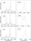 |
Fig. A.1. Three specific examples of the complex [O III] shapes seen in (a) SDSS J013706.95-090857.4, (b) SDSS J163453.66+231242.6 and (c) SDSS J165121.88+215526.2 objects. The complex shape decomposition is shown in left side of figures, where the core components are denoted with dashed line, and multiple Gaussians which sum gives the outflow component, with solid line. The outflow components for [O III]λ 5007 Å are shown separately, in right side of Figures (a1, b1, c1), where vertical dashed line represents zero velocity shift. |
Bae & Woo (2016) gave the 3D models of biconical outflows combined with a thin dust plane. Using a set of input parameters, they found that intrinsic outflow velocity, bicone inclination, and the amount of dust extinction mainly determine the simulated velocity and velocity dispersion of the outflow components. Also, they simulated the emission line profiles for various combinations of the input parameters, giving the diversity of the possible outflow emission shapes.
The observed complex profile of the [O III] outflow component shown in Fig. A.1a is very similar to simulated line profiles given by biconical outflow model for included effects of the dust extinction and angle of bicone inclination i = ±30° (see Fig. 9 in Bae & Woo 2016). In this case, model predicts that dust obscures a part of the bicone, so the emission line flux arising from the outflow offsets from zero velocity, showing asymmetric profiles. Interestingly, the complex line profile shown in Fig. A.1b, with double-peak outflow emission is also predicted by biconical model for the case with no dust extinction and with the outer opening angle of the bicone smaller than absolute value of the angle of bicone inclination, i (see Fig. 11 in Bae & Woo 2016). However, the complex line profile shown in Fig. A.1c, with outflow emission composed from two components, with smaller one extremely blueshifted, is not presented in simulated spectra. The blueshift of the higher Gaussian is −370 km s−1, while smaller component is blueshifted −1810 km s−1. It is possible that this complex outflow shape represent the projection of the two independent, spatially separated outflows.
A.1. The decomposition of the [N II]+ Hα with complex outflow shape
Here we give an example of a possible decomposition of the blended [N II]+ Hα for objects with a complex outflow shape observed in [O III] lines. We chose the object SDSS J013706.95-090857.4 (shown in Fig. A.1a), because it is frequently analysed in the literature, and has a complex outflow shape which is the most common in this sample.
The complex shape of outflow emission in [O III] for this object is approximately described as sum of the two Gaussians (see Fig. A.1a1), so we adopted that shape for outflow components of Hα and [N II] lines. We found intensity ratio of these two Gaussians within one [O III] line, and also the difference between their shifts and widths. In this way we describe complex shape shown in Fig. A.1a1 with only three free parameters: width, shift and intensity of the higher Gaussian, while smaller Gaussian is reproduced relative to higher one. Similarly as done in fitting procedure described in Section 3.4, we fixed Hα and [N II] outflow components to have the same shift and width, but different intensities. Finally, we fitted blended Hα+[N II] in this object with three complex outflow components, described with only 4 free parameters (width, shift and intensity of complex outflow shape for Hα and one more intensity for [N II] doublet).
We found that the complex outflow components which give the best fit of the blended Hα+[N II] have 14% smaller width and significantly smaller blueshift comparing the complex outflow component of [O III] (shift of [O III] outflow component peak ∼ − 300 km s−1, of Hα and [N II] ∼ − 30 km s−1), which is in agreement with relationships obtained by analysing the simple Gaussian outflow components (see Fig. 12). The Hβ and [S II] line profiles in this objects show only small blue asymmetry. It is possible that smaller, extended and extremely broad component of the outflow complex shape cannot be resolved for these lines, because it is diluted by the noise. The decomposition of the blended Hα+[N II] is shown in Fig. 15a.
Appendix B: The correlations between Hα and [N II] line components and σ* for the total sample
In Section 3.1 we analyse the influence of the gravitation to the kinematical properties of the different line components for double-Gaussian and single-Gaussian Hα and [N II] lines (see Fig. 6, Table 1). The influence of gravitation to the line shape of these two lines was done only for the unblended subsample in which Hα and [N II] lines were fitted completely independently. However, there is concern that these results could be biased by selection effects, because the objects with the broadest wing components in Hα and [N II] lines are part of the blended subsample. The blended subsample is decomposed using some fitting constrains for wing components (the same widths and shifts for Hα and [N II] wing components, see Section 3.4), while the core components of both lines are fitted with all free parameters. Some spectra from the blended subsample are decomposed to broad Hα and single-Gaussian Hα and [N II] lines, which are also fitted with all free parameters.
Here we investigated the correlations between σ* and Hα/[N II] line components using the total sample (unblended + blended subsample). Similar to the case of the unblended subsample, we find no correlations between the widths of the Hα and [N II] wing components and σ*, and we find significant correlations between the widths of the core components (and single Gaussian lines) and σ*. The coefficient of correlation between σ* and the Hα core components for total sample is r = 0.50, P = 1.8E-15, and between σ* and [N II] core components, r = 0.53, P = 0. The coefficients of correlations between σ* and single Gaussian lines are: r = 0.63, P = 0 for Hα, and r = 0.64, P = 0 for [N II]. The relationships are shown in Figure B.1.
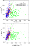 |
Fig. B.1. Correlations between the σ* and velocity dispersion of the single-Gaussian lines (red dots), wing and core components of the double-Gaussian lines (green and blue dots) for Hα and [N II] lines (total sample). The one-to-one relation is denoted with a solid line. |
We can conclude that including the blended subsample in the analysis does not change our basic conclusions about the gravitational influence on the Hα and [N II] line components found for the unblended subsample in Section 3.1.
All Tables
Correlations between the stellar velocity dispersion (σ*) and velocity dispersions of the core components of double-Gaussian lines and single-Gaussian lines.
Correlations between the widths and shifts of the wing components (w) of different lines in the total sample (unblended + blended).
All Figures
|
Fig. 1. Decomposition of the spectrum (SDSS J105621.57−005320.4) into the host galaxy and AGN contributions using SPCA. The black line shows observed data, the red line shows the host galaxy contribution obtained from SPCA, and the blue line shows the AGN contribution (host galaxy contribution subtracted from observed spectrum). |
| In the text | |
|
Fig. 2. (a) Histogram of the distribution of cosmological redshift for the total sample. (b) Histogram of the distribution of [O III]λ 5007 Å luminosity for the total sample (grey bars) and for different subsets (unblended subsample – blue bars, objects from unblended subsample with detected wing components in both Hα and [N II] lines – green bars, and the same but for [N II] and [S II] lines – red bars. |
| In the text | |
|
Fig. 3. [N II]+Hα wavelength band in spectra which belong to the (a) unblended and (b) blended subsamples (SDSS J100551.19+125740.6 and SDSS J112408.63−010927.9, respectively). |
| In the text | |
|
Fig. 4. Example of fit decomposition for object SDSS J125025.82+001954.9 from the unblended subsample: (a) Hα and [N II], (b) Hβ and [O III], and (c) [S II]. The core components are denoted with a dotted line and the wing components with a solid line. |
| In the text | |
|
Fig. 5. Correlations between σ* and the widths of single-Gaussian lines (red dots), and the wing and core components of the double-Gaussian lines (green and blue dots) for [O III], [S II], and Hβ lines (total sample). The one-to-one relation is denoted with the solid line. |
| In the text | |
|
Fig. 6. Same as in Fig. 5, but for Hα and [N II] lines. The correlations are shown for the ‘unblended’ subsample, where Hα and [N II] lines are fitted independently. The one-to-one relation is denoted with a solid line. |
| In the text | |
|
Fig. 7. Histogram of the width distribution of the single-Gaussian [S II] lines and the core components of the double-Gaussian [S II] lines. |
| In the text | |
|
Fig. 8. Correlations between the shifts of the [N II], [S II], and Hα wing components in the unblended subsample (r – coefficient of correlation, and appropriate P-value are given). The data are fitted with a linear function Y = k ⋅ X + n (solid line), where k is the slope and n the intercept of the best linear fit. The one-to-one relation is denoted with a dashed line. The shaded region corresponds to the 95% confidence interval. |
| In the text | |
|
Fig. 9. Correlations between the widths of the [N II] and Hα wing components in the unblended subsample. Notation is the same as in Fig. 8. |
| In the text | |
|
Fig. 10. Example of decomposition of objects from the blended subsample (group a): SDSS J010946.70+134411.9 (a1, b1, c1) and SDSS J111848.44+280738.3 (a2, b2, c2). The blended Hα+[N II] is decomposed as: nested Hα BLR and three weak wing components in panel a1 and with three strong wing components in panel a2. The decomposition of the [O III] and Hβ is shown in panel b1 and b2, and decomposition of the [S II] lines is shown in panels c1 and c2. The core and wing components are denoted with the dotted and solid line, respectively. |
| In the text | |
|
Fig. 11. Example of the complex decomposition of the [N II]+Hα wavelength band for object (SDSS J032525.36−060837.8) with a distinctly extended Hα BLR component (group b). The [N II]+Hα is decomposed into the [N II] and Hα core and wing components, and one Hα BLR component. The core components are denoted with the dotted line, and wing components and Hα BLR are shown with a solid line. |
| In the text | |
|
Fig. 12. Correlation between the shifts (top) and widths (bottom) of the [O III] and Hα wing components for the total sample. The unblended subsample is denoted with full circles and the blended subsample with open circles. The Pearson coefficient of correlation (r), P-value, slope (k), and intercept (n) of the best linear fit (solid line) are given. The dashed line represents the one-to-one relation and the shaded region corresponds to the 95% confidence interval. |
| In the text | |
|
Fig. 13. Correlations between the shift of the Hβ wing components and the shifts of the [O III] (top) and Hα (bottom) wing components for the total sample. The notation is the same as in Fig. 8. |
| In the text | |
|
Fig. 14. Mean profiles of [O III], [N II], Hα, and [S II] wing components for the unblended subsample (a). The mean profiles of the [O III] and Hα wing components for the blended subsample (b). |
| In the text | |
|
Fig. 15. Decomposition of the blended Hα+[N II] for object with a complex shape of the [O III] outflow emission (SDSS J013706.95−090857.4, see Fig. A.1a). The decomposition is done with (a) the sum of the three complex outflow components of the Hα and [N II] doublet, with the same shape as in [O III] lines (see Fig. A.1a1); and (b) with a single broad Gaussian with FWHM ∼ 2600 km s−1. The core components are denoted with a dashed line, and outflow components/broad Gaussian with a solid line. |
| In the text | |
|
Fig. A.1. Three specific examples of the complex [O III] shapes seen in (a) SDSS J013706.95-090857.4, (b) SDSS J163453.66+231242.6 and (c) SDSS J165121.88+215526.2 objects. The complex shape decomposition is shown in left side of figures, where the core components are denoted with dashed line, and multiple Gaussians which sum gives the outflow component, with solid line. The outflow components for [O III]λ 5007 Å are shown separately, in right side of Figures (a1, b1, c1), where vertical dashed line represents zero velocity shift. |
| In the text | |
|
Fig. B.1. Correlations between the σ* and velocity dispersion of the single-Gaussian lines (red dots), wing and core components of the double-Gaussian lines (green and blue dots) for Hα and [N II] lines (total sample). The one-to-one relation is denoted with a solid line. |
| In the text | |
Current usage metrics show cumulative count of Article Views (full-text article views including HTML views, PDF and ePub downloads, according to the available data) and Abstracts Views on Vision4Press platform.
Data correspond to usage on the plateform after 2015. The current usage metrics is available 48-96 hours after online publication and is updated daily on week days.
Initial download of the metrics may take a while.