| Issue |
A&A
Volume 659, March 2022
|
|
|---|---|---|
| Article Number | A19 | |
| Number of page(s) | 8 | |
| Section | Galactic structure, stellar clusters and populations | |
| DOI | https://doi.org/10.1051/0004-6361/202140710 | |
| Published online | 28 February 2022 | |
Introducing a new multi-particle collision method for the evolution of dense stellar systems
II. Core collapse
1
Dipartimento di Fisica e Astronomia & CSDC, Università di Firenze, Via G. Sansone 1, 50019 Sesto Fiorentino, Italy
e-mail: This email address is being protected from spambots. You need JavaScript enabled to view it.
, This email address is being protected from spambots. You need JavaScript enabled to view it.
2
INFN – Sezione di Firenze, Via G. Sansone 1, 50019 Sesto Fiorentino, Italy
3
CREF, Via Panisperna 89A, 00184 Rome, Italy
4
Center for Astro, Particle and Planetary Physics (CAP 3), New York University, Abu Dhabi, UAE
e-mail: This email address is being protected from spambots. You need JavaScript enabled to view it.
5
Department of Astronomy and Center for Galaxy Evolution Research, Yonsei University, Seoul 120-749, Republic of Korea
Received:
3
March
2021
Accepted:
14
June
2021
Abstract
Context. In a previous paper we introduced a new method for simulating collisional gravitational N-body systems with linear time scaling on N, based on the multi-particle collision (MPC) approach. This allows us to easily simulate globular clusters with a realistic number of stellar particles (105 − 106) in a matter of hours on a typical workstation.
Aims. We evolve star clusters containing up to 106 stars to core collapse and beyond. We quantify several aspects of core collapse over multiple realizations and different parameters while always resolving the cluster core with a realistic number of particles.
Methods. We run a large set of N-body simulations with our new code MPCDSS. The cluster mass function is a pure power law with no stellar evolution, allowing us to clearly measure the effects of the mass spectrum on core collapse.
Results. Leading up to core collapse, we find a power-law relation between the size of the core and the time left to core collapse. Our simulations thus confirm the theoretical self-similar contraction picture but with a dependence on the slope of the mass function. The time of core collapse has a non-monotonic dependence on the slope, which is well fitted by a parabola. This also holds for the depth of core collapse and for the dynamical friction timescale of heavy particles. Cluster density profiles at core collapse show a broken-power-law structure, suggesting that central cusps are a genuine feature of collapsed cores. The core bounces back after collapse, with visible fluctuations, and the inner density slope evolves to an asymptotic value. The presence of an intermediate-mass black hole inhibits core collapse, making it much shallower, irrespective of the mass-function slope.
Conclusions. We confirm and expand on several predictions of star cluster evolution before, during, and after core collapse. Such predictions were based on theoretical calculations or small-size direct N-body simulations. Here we put them to the test in MPC simulations with a much larger number of particles, allowing us to resolve the collapsing core.
Key words: globular clusters: general / methods: numerical
© ESO 2022
1. Introduction
Following an initial formation phase from a collapsing parent cloud (Krumholz et al. 2019; Krause et al. 2020), star clusters that survive early gas expulsion (see e.g., Pang et al. 2020) undergo a secular quasi-equilibrium evolution. An initial core contraction phase is ended by a watershed moment, when core collapse halts and reverses as binary burning begins (Giersz & Heggie 1994a,b; Baumgardt et al. 2002; Gieles et al. 2010; Alexander & Gieles 2012). The dynamics of the following gravothermal oscillations (Sugimoto & Bettwieser 1983; Goodman 1987; Allen & Heggie 1992) was found to be characterized by a low-dimensionality chaotic attractor (Breeden & Cohn 1995, and references therein). More generally, the origin and implications of core collapse have historically been studied both analytically (Ambartsumian 1938; Spitzer 1940; Chandrasekhar 1942; Hénon 1961; Lynden-Bell & Wood 1968; Heggie 1979a,b) and through simulations (Larson 1970; Spitzer & Shull 1975; Hénon 1975; Baumgardt et al. 2003); an early review of both is available in Meylan & Heggie (1997). Once the importance of core collapse had been established, a large body of work was carried out on the subject of star-cluster evolution all the way to core collapse and beyond; this work strongly relied on direct N-body simulations, with N increasing over the years as hardware capabilities improved (see e.g. Spurzem & Aarseth 1996; Makino 1996; Baumgardt & Makino 2003; Trenti et al. 2010; Hurley & Shara 2012; Sippel et al. 2012; Heggie 2014). The time complexity of direct N-body simulations is, however, at least quadratic (e.g. Aarseth 1999; Harfst et al. 2007). Thanks to parallel codes running on graphics processing units (Wang et al. 2015), current simulations reach N ≈ 106, but this still requires several thousand hours on a dedicated computer cluster (Wang et al. 2016; see also e.g. Heggie 2011 and references therein), with very recent N-body codes mitigating this issue (Wang et al. 2020) without changing the overall scaling behaviour. This makes replication of any given numerical experiment impractical and forces researchers to rely, at best, on just a few realizations of a given system.
While open clusters can essentially be simulated with a 1:1 ratio between real stars and simulation particles, the fact that large direct N-body simulations are impractical has detrimental implications for modelling globular clusters (except perhaps the smaller ones) and larger systems, such as nuclear star clusters. It was realized very early on (Goodman 1987) that tacitly assuming that we can scale up the results of small direct N-body simulations by one or more orders of magnitude is dangerous as post-collapse dynamical behaviour can become qualitatively different with increasing numbers of particles. In addition, even if the rescaled crossing times are equal, direct simulations with a substantially different number of particles have significantly different effective two-body relaxation times that explicitly depend on the number of particles, N, as N/log(N). As already recognized in the context of cosmological simulations (e.g. see Binney & Knebe 2002; Diemand et al. 2004; El-Zant 2006), this might lead to large differences in the end states of two simulations that represent the ‘same’ system of total mass, M, with different numbers of particles. In particular, all instability processes associated with discreteness effects will set up at earlier times (in units of a given dynamical time as a function of a fixed mean mass density  ,
,  ) when a smaller number of particles is used in the simulation.
Moreover, low-N simulations that include an intermediate-mass black hole (IMBH) of mass MIMBH in a star cluster core of mass Mcore with average stellar mass ⟨m⟩ are bound to be unrealistic, either underestimating the MIMBH/⟨m⟩ ratio or overestimating the MIMBH/Mcore ratio because Mcore/⟨m⟩ is the (unrealistically low) number of stars included in the simulated core. By doing so, for example, the dynamical friction timescale for a displaced black hole sinking back into the star cluster core might be significantly altered, thus leading to potentially wrong conclusions on the dynamics of the cluster itself. A smaller number of simulation particles at a fixed total cluster mass also affects the formation of the loss cone since this formation is primarily governed by the mass ratio between the black hole and the stars.
Alternatives to direct N-body simulations are approximate methods, typically based on solving the Fokker-Planck equation (e.g., Hypki & Giersz 2013, for a state-of-the-art Monte Carlo solver), resulting in dramatically shorter run times. In a previous paper (Di Cintio et al. 2021, henceforth D2020) we introduced a code for simulating gravitational N-body systems, called MPCDSS, that takes a new approach to approximating collisional evolution through the so-called multi-particle collision (MPC) method. We refer the reader to D2020 for details on the method, its rationale, and its implementation. In the present paper we focus on using our code to simulate star clusters containing up to 106 particles through core collapse, calculating several indicators of the cluster’s dynamical state and comparing with theoretical expectations. Because our typical simulation takes no more than a few hours on an ordinary workstation, we can run multiple realizations of any given system and explore the relevant parameter space at leisure, in particular exploring the effect of varying the mass-function slope. In order to achieve additional speed-up and simplify the numerical simulations, in the implementation of MPCDSS used here we neglect stellar evolution1, both single and binary. While for now we do not model binaries, they will be included in an upcoming version of the code (Di Cintio et al., in prep.). While these choices reduce the numerical complexity of the simulations at the expense of some loss of realism, they also allow us to disentangle the purely dynamical causes of several specific phenomena from those due to, for example, stellar evolution; this facilitates comparisons with purely theoretical works.
2. Simulations
2.1. Initial conditions
We ran a set of hybrid particle-mesh-MPC simulations using the newly introduced MPCDSS code (in D2020 we compared this method to direct N-body simulations, showing similar results despite dramatically shorter run times) on an eight-core workstation. The number of simulation particles ranges from 104 to 106, initially distributed following the Plummer (1911) profile,
 (1)
(1)
of total mass, M, and scale radius, rs. The mass function is a pure power-law mass of the form
 (2)
(2)
of which Salpeter (1955) is a special case corresponding to α = 2.3, and where the normalization constant C depends on the minimum-to-maximum-mass ratio ℛ = mmin/mmax, so that  .
.
In the simulations presented in this work we concentrate on the three values of ℛ = 10−2, 10−3, and 10−4. The exponent α spans from 0.6 to 3.0 in increments of 0.1. The systems evolve in isolation, stellar evolution is turned off, and the primordial binary fraction is always set to zero.
2.2. Numerical scheme
In line with D2020, we evolved all sets of simulations for about 104 dynamical times,  , so that in all cases the systems reach core collapse and are evolved further after it for at least another 103tdyn. We employed our recent implementation of MPCDSS, in which the collective gravitational potential and force are computed by standard particle-in-cell schemes on a fixed spherical grid of Ng = Nr × Nϑ × Nφ mesh points, while the inter-particle (dynamical) collisions are resolved using the so-called MPC scheme (see Malevanets & Kapral 1999).
In the simulations presented here, we have solved the Poisson equation ΔΦ = −4πGρ using a fixed mesh with Nr = 1024, Nϑ = 16, and Nφ = 16 with logarithmically spaced radial bins extended up to 100rs2 with the spherical particle mesh method from Londrillo & Messina (1990). Since the systems under consideration are supposed to maintain their spherical symmetry, we averaged the potential Φ along the azimuthal and polar coordinates in order to reduce the small-N noise in scarcely populated cells and enforce the spherical symmetry throughout the simulation.
The MPC (see Di Cintio et al. 2017 and D2020 for further details) essentially consists of a cell-dependant rotation of particle velocities in the cell’s centre of mass frame moving at ucom in the simulation’s frame, which, for the jth particle of velocity vj in cell i, reads
 (3)
(3)
In the above equation, Ri is a random rotation axis, δvj = vj − ui, and δvj, ⊥ and δvj, ∥ are the relative velocity components perpendicular and parallel to Ri, respectively. The rotation angle αi when chosen randomly yields an MPC rule that only preserves kinetic energy and momentum. If it is fixed by a particular function of particles (again, see D2020 for the details), positions in the simulation frame and velocities in the centre-of-mass frame also allow one to preserve one of the components of the angular momentum vector.
In the simulations discussed in this work, the MPC operation was performed on a different polar mesh with respect to that of the potential calculation, with Ng = 32 × 16 × 16 points, extended only up to rcut = 20rs. By doing so, particles at larger radii (thus in a region where the density is extremely low) are not affected by collisions.
In all the simulations presented here we used the same normalization such that G = M = rs = tdyn = 1. In these units we adopted a constant time step, Δt = 10−2, that always ensures a good balance between accuracy and computational cost.
In the runs that included the central IMBH, its interaction with the stars was evaluated directly (i.e. the IMBH does not take part in the MPC step nor in the evaluation of the mean field potential). In order to keep the same rather large Δt of the simulation, the potential exerted by the IMBH was smoothed as  , where we took ϵ = 10−4 in units of rs so that, for the IMBH mass-to-cluster mass ratio 10−3, the softening length is always of the order of one-tenth of the influence radius of the IMBH.
3. Results
3.1. Evolution before core collapse
We defined the time of core collapse, tcc, as the time at which the 3D radius containing the most central 2% of the simulation’s particles reaches its absolute minimum. In the following we refer to this as the Lagrangian radius r2%. The 2% radius is small enough to track the dynamics of the innermost parts of the core while still including enough particles to be relatively unaffected by shot noise. We also calculated the 3D Lagrangian radii, rL(t), enclosing different fractions of the total number of particles, N, ranging from the 2% to the 90%. We track the evolution of our simulations towards core collapse both through these radii and the central mass density,  . The latter is defined as the mean 3D mass density within 5% of the scale radius of our initial Plummer model (i.e. rm = 0.05rs).
The evolution of  and the selected Lagrangian radii are presented in the upper and lower panels of Fig. 1, respectively, for the runs with ℛ = 10−3, N = 2 × 10⁵, and α = 0.6, 1.0, 1.5, 2.0, 2.3, 2.5, and 3.0. In all simulations the central density increases monotonically (modulo fluctuations) with time until a maximum, corresponding to core collapse, is reached. The slope of the mass function determines both the time at which maximum density is reached and the characteristics of the density growth before this maximum, with α = 1.5 acting as a watershed between concave and convex evolution (in log-log scale; see Fig. 1). In general, in models associated with larger values of α the central density increases more and more rapidly and settles to a somewhat constant value after core collapse, when the inner Lagrangian radii are already re-expanding. We compare this behaviour to a simplified, equal-mass, self-similar collapse model such as the one presented in chapter 3.1 of Spitzer (1987) (but see also Lynden-Bell & Eggleton 1980 and the following discussion), which predicts a monotonic growth of density with time, generally with positive curvature. Clearly, the presence of a mass spectrum in our simulations introduces an additional degree of freedom, complicating the behaviour of the system3. In particular, the presence of a mass spectrum implies that, as the core collapse sets in, the system is also undergoing mass segregation. The latter happens at different rates depending on the structure of the mass spectrum itself since different masses might in principle have different dynamical friction timescales. In fact, Ciotti (2010, 2021) found that in (infinitely extended) models with exponential or power-law mass spectra, the strength of the dynamical friction coefficient, ν, is heavily affected by the mass distribution for test particles with masses comparable with the mean mass, ⟨m⟩, being larger by up to a factor of ten with respect to the classical case.
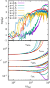 |
Fig. 1. Core density, |

All of our simulations undergo core collapse within, at most, four initial two-body relaxation times (defined as t2b = 0.138Ntdyn/log N). From Fig. 1 it appears that the evolutionary paths of Lagrangian radii are similar across various realizations with the same ℛ and N but different α. In other words, our simulated star clusters expand in average size monotonically with relatively little dependence on the mass spectrum. This spectrum instead has a clear influence on the evolution of the core as described by the innermost Lagrangian radii, which contract with noticeably different patterns for different values of α. Lynden-Bell & Eggleton (1980) calculated analytically the time evolution of a cluster’s core radius, rc, in the phases leading to core collapse within the context of a self-similar collapse scenario:
 (4)
(4)
where 2 < μ < 2.5. Our simulations are in qualitative agreement with the analytical predictions of Lynden-Bell & Eggleton (1980) in the initial phase of core collapse, regardless of the specific number of particles and mass ratios, for α ≲ 1.5. In Fig. 2 we show the power-law dependence of the 2% Lagrangian radius on the time left to core collapse (tcc − t) for α = 0.6, 0.8, 1.0, 1.2, 1.4, and 1.6 with N = 2 × 10⁵ and ℛ = 10−3, which appears as a linear relation in our log-log plot.
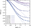 |
Fig. 2. Power-law dependence between core size (r2% 3D Lagrangian radius) and time left to core collapse, tcc − t. A power-law relation (appearing linear in log-log scale) holds in the initial phases of core collapse. We show it here for models with mass-function slope α = 0.6, 0.8, 1.0, 1.2, 1.4, and 1.6, number of stars N = 2 × 10⁵, and ℛ = 10−3. Due to our definition of the x axis, time increases from right to left. The solid lines are data from our simulations, and the superimposed dashed lines are a robust linear fit between the initial time and tcc − 100tdyn. The angular coefficient of the regression lines appears to vary systematically with the mass function. As expected, the power-law relation breaks before core collapse, when the self-similar contraction phase ends. |
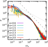 |
Fig. 3. Double power-law 3D density profile at tcc for models with α = 0.6, 1.0, 1.5, 2.0, 2.3, 2.5, and 3.0, N = 2 × 10⁵, and ℛ = 10−3. The initial isotropic Plummer profile is shown as a solid thin black line. The dashed and dotted lines mark the inner and outer limit trends (ρ ∼ r−1.5 and ∼r−3 of the core density, respectively). |
For higher values of α, for which the core collapse happens over a few hundred tdyn, it becomes harder to fit a linear relation due to insufficient data points. Departure from the results of Lynden-Bell & Eggleton (1980) is expected to happen in the late stages of core collapse due to energy generation mechanisms in the cluster’s core; this is indeed observed in Fig. 2, which shows a proportionality between log r2% and log(tcc − t) up until log r2% saturates to a constant value as the core stops contracting.
However, the slope of this power-law relation depends on the initial mass function of our simulation, so Eq. (4) cannot hold with a constant μ over our whole set of simulations. This discrepancy is not surprising given that Lynden-Bell & Eggleton (1980) used an equal-mass approximation. The mass spectrum appears to have a twofold effect on the dynamics of core collapse. First, for a fixed total mass and density profile, it affects the rate at which the (quasi-)self-similar contraction happens, and second it dictates different times at which such contraction departs from self-similarity (e.g. see Khalisi et al. 2007). In particular, models with shallower mass spectra (i.e. smaller α) have much longer self-similar collapse phases. We interpret this fact as an effect of the competition between mass segregation and core collapse itself.
In order to investigate the process of mass segregation in a multi-mass system, we time-dependently computed the indicator ϕmr, defined as
 (5)
(5)
In the above equation, ⟨x⟩ is the mean value of the quantity x within a given Lagrangian radius. This indicator can be understood as the mass-weighted mean radius divided by the mean radius. Since all initial conditions used in this work are characterized by position-independent mass spectra, ϕmr = 1 at all radii at t = 0. As the systems evolve, with heavier stars sinking at smaller radii, r, we expect ϕmr to decrease (at least when computed for Lagrangian radii smaller than roughly r50%).
We evaluated ϕmr inside different Lagrangian radii, finding that the models remain essentially non-segregated up to roughly 100tdyn, while at later times, with different rates, the energy exchanges mediated by the collisions lead to a concentration of heavier stars in the inner regions of the systems. As an example, in Fig. 4 we show the time evolution of the segregation indicator for the α = 0.6, 1.0, 2.3, and 3.0 cases with ℛ = 10−3. Remarkably, in all cases, ϕmr settles to a reasonably constant value for a few thousand dynamical times before changing appreciably, while in the same time window the corresponding Lagrangian radii are already rapidly re-expanding (compare with Fig. 1).
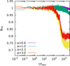 |
Fig. 4. Time evolution of the mass segregation indicator, ϕmr, computed within r2% for models with α = 0.6, 1.0, 2.3, and 3.0 and ℛ = 10−3. |
In Fig. 5 we show instead the time, tms, at which the mass segregation starts to take place (i.e. when ϕmr starts to depart sensibly from 1) as a function of the mass spectrum exponent, α. We find that such a mass segregation timescale decreases monotonically for increasing α, while the final value of ϕmr has a non-monotonic trend with α.
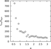 |
Fig. 5. Time of the mass segregation onset, tms, in units of tdyn, as a function of the mass spectrum slope, α, for the models with ℛ = 10−3. |
3.2. Density profile at core collapse: Broken power law
Starting from a flat-cored Plummer initial condition, the functional form of the density profile undergoes in all cases a dramatic evolution before and after the core collapse. For all explored values of α and ℛ, the density profile at the time of core collapse, tcc, presents a multiple power-law structure, as shown in Fig. 3 for α = 0.6, 1.0, 1.5, 2.0, 2.3, 2.5, and 3.0 and ℛ = 10−3. Such a multiple power-law structure is also observed in some Galactic globular clusters for which cores were resolved using the Hubble Space Telescope (e.g. Noyola & Gebhardt 2007) and is often regarded as an indication of core collapse (see Trenti et al. 2010; Vesperini & Trenti 2010, for a discussion based on direct N-body simulations). Typically, lower values of α are associated with steeper central density profiles, with both core and outer density slopes, γint and γext, between −1.5 and −3.
In Fig. 6 we show that, remarkably, the evolution of the density profile for α ≳ 1.5 leads at later times to a central density slope compatible with γ ∼ −2.23. This holds true regardless of the specific value of α and is in agreement with what was found by Hurley & Shara (2012), Giersz et al. (2013), Pavlík & Šubr (2018), and D2020. This essentially coincides with the slope value γ ∼ −2.21 found by Lynden-Bell & Eggleton (1980) using a heat conduction approximation to the energy transport mediated by stellar encounters.
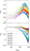 |
Fig. 6. Evolution of the 3D density slope, γ, between r50% and r80% (top panel) and between r10% and r50% (bottom panel) for the models with α = 0.6, 1.0, 1.5, 2.0, 2.3, 2.5, and 3.0, N = 2 × 10⁵, and ℛ = 10−3. The horizontal dashed line in the bottom panel marks the asymptotic slope, γ = −2.23. |
3.3. Time and depth of core collapse
As stated above, for each simulation we took the time of core collapse, tcc, as the time at which the minimum value of the r2% 3D Lagrangian radius is achieved. The upper panel of Fig. 7 shows tcc as a function of the initial mass-function power law α.
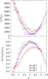 |
Fig. 7. Time of core collapse as a function of the mass-function slope (top panel) and depth of core collapse (bottom panel) for isolated Plummer models with N = 2 × 10⁵ and ℛ = 10−2 (red squares), 10−3 (black circles), and 10−4 (purple triangles). The times are given in units of the dynamical time, tdyn. The solid lines mark our second-order polynomial best fit. |
Simulations starting with a steeper mass function (i.e. higher values of α) are more similar to the equal-mass case and thus reach core collapse at later times (independently of the number of particles and for all mass ratios, ℛ, if time is measured in units of dynamical timescales of the simulation; see also Fig. 7 in D2020). This is expected from well-established theory (e.g. Spitzer 1975) that shows that evolution is sped up by a mass spectrum. In addition to taking longer to reach core collapse, low-α runs also reach shallower values of the core density at tcc.
Still, and interestingly, for α > 2.3 the time of core collapse starts increasing again. The same non-monotonic trend is also observed for the depth of core collapse, dcc, defined as the ratio of r2% at t = tcc to r2% at t = 0 (same figure, bottom panel). We fitted both relations of tcc and dcc with the mass-function exponent α using a second-order polynomial (thin solid lines). As a general trend, for fixed α the core collapse is deeper (i.e. lower values of dcc) and happens at later times for the models with larger minimum-to-maximum-mass ratios, ℛ. This has a similar explanation as the dependence on α since a larger ℛ is more similar to the single-mass case.
In Fig. 8 we plot the dynamical friction timescale for particles with mass 4⟨m⟩, showing that it is relatively unaffected by ℛ but depends on α in a similar fashion as the timescale for core collapse, with a minimum at intermediate values of α in the 2.0 − 2.5 range. The lack of ℛ dependence is due to the fact that changes in ℛ affect only the extremes of the mass spectrum and so are not observed for particles in this relatively central mass range.
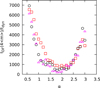 |
Fig. 8. Estimated dynamical friction time, tDF, for particles with mass 4⟨m⟩ as a function of the mass spectrum slope, α, for models with N = 2 × 10² and ℛ = 10−2 (squares), 10−3 (circles), and 10−4 (triangles). |
3.4. Effects of an IMBH
In Fig. 9 we show the evolution of central density and Lagrangian radii for three simulations containing 106 particles, α = 2.3, and an initially central IMBH of three different masses, 3 × 10⁻⁴, 10−3, and 3 × 10⁻³, the total simulation mass. Because N = 106, the mass ratio between the IMBH and a typical star is within the correct astrophysical range for a typical globular star cluster, assuming that the mass of an IMBH ranges from 102 to 105 M⊙ (e.g. see Greene et al. 2020) and that the stars in globular clusters have an average mass of ≈0.5 M⊙. In all cases the core collapse stops at earlier times for the models with a central IMBH with respect to the cases without an IMBH; however, it is generally much shallower, involving, at most, a contraction of the Lagrangian radius r2% of roughly 10%, after which the core size bounces back quickly and expands far more than in systems that do not host a central IMBH. We thus confirm the theoretical expectations that IMBHs induce swollen cores in star clusters (see e.g. Hurley 2007; Umbreit et al. 2008, 2012, and references therein).
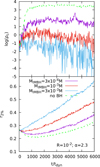 |
Fig. 9. Time evolution of the mean central density, |

4. Discussion and conclusions
We used a new N-body simulation approach based on the MPC method to simulate star clusters with a realistic number of particles, from 105 up to 106. We simulated systems characterized by a power-law mass function, whose exponent was varied in small increments over a wide range of values, resulting in 98 different initial conditions (summarized in Table 1). This was made possible by the high performance of our code when compared to a direct N-body approach (with linear complexity versus quadratic in the number of particles).
Parameters of the initial conditions for our runs.
We found that, for all slopes of the mass spectrum we simulated, the 3D density profile at core collapse has a broken-power-law shape. This suggests that a central density cusp may be an indication of core-collapsed status in real star clusters. Thanks to the large number of particles we could simulate using our new technique, we were able to resolve this power-law cusp deep into the innermost regions of the core. Among other findings that confirm previous analytical work, we have shown that the slope of this inner cusp evolves asymptotically to the value predicted by Lynden-Bell & Eggleton (1980) based on an analytical model. Additionally, our simulations evolve through the initial self-similar phase of core collapse (before binary burning kicks in), following the Lynden-Bell & Eggleton (1980) prediction (originally developed for a single-mass system) of a power-law scaling of core radius with time to core collapse, despite the scaling law we observe having a different exponent that depends on the chosen mass spectrum. Remarkably, such a power-law behaviour is retrieved even though binary formation has been neglected in the set of simulations presented here.
We find a somewhat surprising parabolic dependence of the time and depth of core collapse as a function of the mass-function slope. This is likely caused by the similarly non-monotonic dependence of the dynamical friction timescale on said slope, as we plan to show analytically within the framework introduced by Ciotti (2010).
Finally, we were able to simulate 106 particle star clusters that included an IMBH, thus correctly matching the MIMBH/⟨m⟩ ratio, which is currently at the limit of direct N-body simulation capabilities. We confirm previous results, showing that an IMBH essentially induces a faster and shallower core collapse that reverts rapidly, resulting in an appreciably swollen core, with respect to models with the same initial mass distribution but without an IMBH.
We note that including stellar evolution in a particle-based simulator for globular clusters costs only an order N increase in computational time, the bottleneck of the integration always being the evaluation of the gravitational forces, scaling, at best, as Nlog(N).
Particles outside that radius are influenced by the monopole 1/r term of the mass distribution.
In D2020 (Fig. 6) we show that the cumulative number of escapers is a largely linear function of time, irrespective of the slope of the mass function, α. Under this condition, the only free parameter in the model, ζ, presented in chapter 3.1 of Spitzer (1987), is fully determined, yielding a constant density as a function of time. In particular, Eq. (3.6) of Spitzer (1987) sets ζ = 5/3, so the power-law exponent in Eq. (3.8) becomes 0.
Acknowledgments
M.P. acknowledges financial support from the European Union’s Horizon 2020 research and innovation programme under the Marie Sklodowska-Curie grant agreement No. 896248. M.P. contribution to this material is based upon work supported by Tamkeen under the NYU Abu Dhabi Research Institute grant CAP3. P.F.D.C. and A.S.-P. wish to thank the financing from MIUR-PRIN2017 project Coarse-grained description for non-equilibrium systems and transport phenomena (CO-NEST) n.201798CZL. S.-J.Y. acknowledges support by the Mid-career Researcher Program (No.2019R1A2C3006242) and the SRC Program (the Center for Galaxy Evolution Research; No. 2017R1A5A1070354) through the National Research Foundation of Korea. We thank the anonymous Referee for his/her comments that helped improving the presentation of our results.
References
- Aarseth, S. J. 1999, PASP, 111, 1333 [NASA ADS] [CrossRef] [Google Scholar]
- Alexander, P. E. R., & Gieles, M. 2012, MNRAS, 422, 3415 [NASA ADS] [CrossRef] [Google Scholar]
- Allen, F. S., & Heggie, D. C. 1992, MNRAS, 257, 245 [NASA ADS] [CrossRef] [Google Scholar]
- Ambartsumian, V. A. 1938, TsAGI Uchenye Zapiski, 22, 19 [NASA ADS] [Google Scholar]
- Baumgardt, H., & Makino, J. 2003, MNRAS, 340, 227 [NASA ADS] [CrossRef] [Google Scholar]
- Baumgardt, H., Hut, P., & Heggie, D. C. 2002, MNRAS, 336, 1069 [NASA ADS] [CrossRef] [Google Scholar]
- Baumgardt, H., Heggie, D. C., Hut, P., & Makino, J. 2003, MNRAS, 341, 247 [NASA ADS] [CrossRef] [Google Scholar]
- Binney, J., & Knebe, A. 2002, MNRAS, 333, 378 [NASA ADS] [CrossRef] [Google Scholar]
- Breeden, J. L., & Cohn, H. N. 1995, ApJ, 448, 672 [NASA ADS] [CrossRef] [Google Scholar]
- Chandrasekhar, S. 1942, in Principles of Stellar Dynamics (University of Chicago Press) [Google Scholar]
- Ciotti, L. 2010, in Amer. Inst. Phys. Conf. Series, eds. G. Bertin, F. de Luca, G. Lodato, R. Pozzoli, & M. Romé, 1242, 117 [NASA ADS] [Google Scholar]
- Ciotti, L. 2021, Introduction to Stellar Dynamics (Cambridge University Press) [CrossRef] [Google Scholar]
- Di Cintio, P., Livi, R., Lepri, S., & Ciraolo, G. 2017, Phys. Rev. E, 95, 043203 [NASA ADS] [CrossRef] [Google Scholar]
- Di Cintio, P., Pasquato, M., Kim, H., & Yoon, S.-J. 2021, A&A, 649, A24 [NASA ADS] [CrossRef] [EDP Sciences] [Google Scholar]
- Diemand, J., Moore, B., Stadel, J., & Kazantzidis, S. 2004, MNRAS, 348, 977 [Google Scholar]
- El-Zant, A. A. 2006, MNRAS, 370, 1247 [NASA ADS] [CrossRef] [Google Scholar]
- Gieles, M., Baumgardt, H., Heggie, D. C., & Lamers, H. J. G. L. M. 2010, MNRAS, 408, L16 [NASA ADS] [CrossRef] [Google Scholar]
- Giersz, M., & Heggie, D. C. 1994a, MNRAS, 268, 257 [NASA ADS] [CrossRef] [Google Scholar]
- Giersz, M., & Heggie, D. C. 1994b, MNRAS, 270, 298 [NASA ADS] [CrossRef] [Google Scholar]
- Giersz, M., Heggie, D. C., Hurley, J. R., & Hypki, A. 2013, MNRAS, 431, 2184 [NASA ADS] [CrossRef] [Google Scholar]
- Goodman, J. 1987, ApJ, 313, 576 [NASA ADS] [CrossRef] [Google Scholar]
- Greene, J. E., Strader, J., & Ho, L. C. 2020, ARA&A, 58, 257 [Google Scholar]
- Harfst, S., Gualandris, A., Merritt, D., et al. 2007, New A, 12, 357 [NASA ADS] [CrossRef] [Google Scholar]
- Heggie, D. C. 1979a, MNRAS, 186, 155 [NASA ADS] [CrossRef] [Google Scholar]
- Heggie, D. C. 1979b, MNRAS, 76, 525 [NASA ADS] [CrossRef] [Google Scholar]
- Heggie, D. C. 2011, Problems of Collisional Stellar Dynamics (World Scientific Publishing), 121 [Google Scholar]
- Heggie, D. C. 2014, MNRAS, 445, 3435 [NASA ADS] [CrossRef] [Google Scholar]
- Hénon, M. 1961, Ann. Astrophys., 24, 369 [Google Scholar]
- Hénon, M. 1975, in Dynamics of the Solar Systems, ed. A. Hayli, 69, 133 [Google Scholar]
- Hurley, J. R. 2007, MNRAS, 379, 93 [CrossRef] [Google Scholar]
- Hurley, J. R., & Shara, M. M. 2012, MNRAS, 425, 2872 [NASA ADS] [CrossRef] [Google Scholar]
- Hypki, A., & Giersz, M. 2013, MNRAS, 429, 1221 [NASA ADS] [CrossRef] [Google Scholar]
- Khalisi, E., Amaro-Seoane, P., & Spurzem, R. 2007, MNRAS, 374, 703 [NASA ADS] [CrossRef] [Google Scholar]
- Krause, M. G. H., Offner, S. S. R., Charbonnel, C., et al. 2020, Space Sci. Rev., 216, 64 [CrossRef] [Google Scholar]
- Krumholz, M. R., McKee, C. F., & Bland-Hawthorn, J. 2019, ARA&A, 57, 227 [NASA ADS] [CrossRef] [Google Scholar]
- Larson, R. B. 1970, MNRAS, 147, 323 [NASA ADS] [Google Scholar]
- Londrillo, P., & Messina, A. 1990, MNRAS, 242, 595 [NASA ADS] [CrossRef] [Google Scholar]
- Lynden-Bell, D., & Eggleton, P. P. 1980, MNRAS, 191, 483 [NASA ADS] [Google Scholar]
- Lynden-Bell, D., & Wood, R. 1968, MNRAS, 138, 495 [NASA ADS] [Google Scholar]
- Makino, J. 1996, ApJ, 471, 796 [NASA ADS] [CrossRef] [Google Scholar]
- Malevanets, A., & Kapral, R. 1999, J. Chem. Phys., 110, 8605 [NASA ADS] [CrossRef] [Google Scholar]
- Meylan, G., & Heggie, D. C. 1997, A&ARv, 8, 1 [NASA ADS] [CrossRef] [Google Scholar]
- Noyola, E., & Gebhardt, K. 2007, AJ, 134, 912 [NASA ADS] [CrossRef] [Google Scholar]
- Pang, X., Li, Y., Tang, S.-Y., Pasquato, M., & Kouwenhoven, M. B. N. 2020, ApJ, 900, L4 [NASA ADS] [CrossRef] [Google Scholar]
- Pavlík, V., & Šubr, L. 2018, A&A, 620, A70 [NASA ADS] [CrossRef] [EDP Sciences] [Google Scholar]
- Plummer, H. C. 1911, MNRAS, 71, 460 [Google Scholar]
- Salpeter, E. E. 1955, ApJ, 121, 161 [Google Scholar]
- Sippel, A. C., Hurley, J. R., Madrid, J. P., & Harris, W. E. 2012, MNRAS, 427, 167 [NASA ADS] [CrossRef] [Google Scholar]
- Spitzer, L. 1987, Dynamical Evolution of Globular Clusters (Princeton, NJ: Princeton University Press), 191 [Google Scholar]
- Spitzer, L. J. 1940, MNRAS, 100, 396 [NASA ADS] [CrossRef] [Google Scholar]
- Spitzer, L. J. 1975, in Dynamics of the Solar Systems, ed. A. Hayli, 69, 3 [NASA ADS] [Google Scholar]
- Spitzer, L. J., & Shull, J. M. 1975, ApJ, 201, 773 [NASA ADS] [CrossRef] [Google Scholar]
- Spurzem, R., & Aarseth, S. J. 1996, MNRAS, 282, 19 [NASA ADS] [CrossRef] [Google Scholar]
- Sugimoto, D., & Bettwieser, E. 1983, MNRAS, 204, 19P [NASA ADS] [Google Scholar]
- Trenti, M., Vesperini, E., & Pasquato, M. 2010, ApJ, 708, 1598 [NASA ADS] [CrossRef] [Google Scholar]
- Umbreit, S., Fregeau, J. M., Chatterjee, S., & Rasio, F. A. 2012, ApJ, 750, 31 [NASA ADS] [CrossRef] [Google Scholar]
- Umbreit, S., Fregeau, J. M., & Rasio, F. A. 2008, in Dynamical Evolution of Dense Stellar Systems, eds. E. Vesperini, M. Giersz, & A. Sills, 246, 351 [NASA ADS] [Google Scholar]
- Vesperini, E., & Trenti, M. 2010, ApJ, 720, L179 [NASA ADS] [CrossRef] [Google Scholar]
- Wang, L., Spurzem, R., Aarseth, S., et al. 2015, MNRAS, 450, 4070 [NASA ADS] [CrossRef] [Google Scholar]
- Wang, L., Spurzem, R., Aarseth, S., et al. 2016, MNRAS, 458, 1450 [Google Scholar]
- Wang, L., Iwasawa, M., Nitadori, K., & Makino, J. 2020, MNRAS, 497, 536 [NASA ADS] [CrossRef] [Google Scholar]
All Tables
All Figures
|
Fig. 1. Core density, |
| In the text | |
|
Fig. 2. Power-law dependence between core size (r2% 3D Lagrangian radius) and time left to core collapse, tcc − t. A power-law relation (appearing linear in log-log scale) holds in the initial phases of core collapse. We show it here for models with mass-function slope α = 0.6, 0.8, 1.0, 1.2, 1.4, and 1.6, number of stars N = 2 × 10⁵, and ℛ = 10−3. Due to our definition of the x axis, time increases from right to left. The solid lines are data from our simulations, and the superimposed dashed lines are a robust linear fit between the initial time and tcc − 100tdyn. The angular coefficient of the regression lines appears to vary systematically with the mass function. As expected, the power-law relation breaks before core collapse, when the self-similar contraction phase ends. |
| In the text | |
|
Fig. 3. Double power-law 3D density profile at tcc for models with α = 0.6, 1.0, 1.5, 2.0, 2.3, 2.5, and 3.0, N = 2 × 10⁵, and ℛ = 10−3. The initial isotropic Plummer profile is shown as a solid thin black line. The dashed and dotted lines mark the inner and outer limit trends (ρ ∼ r−1.5 and ∼r−3 of the core density, respectively). |
| In the text | |
|
Fig. 4. Time evolution of the mass segregation indicator, ϕmr, computed within r2% for models with α = 0.6, 1.0, 2.3, and 3.0 and ℛ = 10−3. |
| In the text | |
|
Fig. 5. Time of the mass segregation onset, tms, in units of tdyn, as a function of the mass spectrum slope, α, for the models with ℛ = 10−3. |
| In the text | |
|
Fig. 6. Evolution of the 3D density slope, γ, between r50% and r80% (top panel) and between r10% and r50% (bottom panel) for the models with α = 0.6, 1.0, 1.5, 2.0, 2.3, 2.5, and 3.0, N = 2 × 10⁵, and ℛ = 10−3. The horizontal dashed line in the bottom panel marks the asymptotic slope, γ = −2.23. |
| In the text | |
|
Fig. 7. Time of core collapse as a function of the mass-function slope (top panel) and depth of core collapse (bottom panel) for isolated Plummer models with N = 2 × 10⁵ and ℛ = 10−2 (red squares), 10−3 (black circles), and 10−4 (purple triangles). The times are given in units of the dynamical time, tdyn. The solid lines mark our second-order polynomial best fit. |
| In the text | |
|
Fig. 8. Estimated dynamical friction time, tDF, for particles with mass 4⟨m⟩ as a function of the mass spectrum slope, α, for models with N = 2 × 10² and ℛ = 10−2 (squares), 10−3 (circles), and 10−4 (triangles). |
| In the text | |
|
Fig. 9. Time evolution of the mean central density, |
| In the text | |
Current usage metrics show cumulative count of Article Views (full-text article views including HTML views, PDF and ePub downloads, according to the available data) and Abstracts Views on Vision4Press platform.
Data correspond to usage on the plateform after 2015. The current usage metrics is available 48-96 hours after online publication and is updated daily on week days.
Initial download of the metrics may take a while.