| Issue |
A&A
Volume 658, February 2022
|
|
|---|---|---|
| Article Number | L8 | |
| Number of page(s) | 11 | |
| Section | Letters to the Editor | |
| DOI | https://doi.org/10.1051/0004-6361/202142684 | |
| Published online | 07 February 2022 | |
Letter to the Editor
Searching for anomalous microwave emission in nearby galaxies
K-band observations with the Sardinia Radio Telescope
1
INAF-Osservatorio Astrofisico di Arcetri, L. E. Fermi 50, 50125 Firenze, Italy
e-mail: This email address is being protected from spambots. You need JavaScript enabled to view it.
2
INAF-Osservatorio Astronomico di Cagliari, Via della Scienza 5, 09047 Selargius, CA, Italy
3
INAF-Istituto di Radioastronomia, Via P. Gobetti, 101, 40129 Bologna, Italy
4
AIM, CEA, CNRS, Université Paris-Saclay, Université Paris Diderot, Sorbonne Paris Cité, 91191 Gif-sur-Yvette, France
5
Université Paris-Saclay, CNRS, Institut d’Astrophysique Spatiale, 91405 Orsay, France
6
National Observatory of Athens, Institute for Astronomy, Astrophysics, Space Applications and Remote Sensing, Ioannou Metaxa and Vasileos Pavlou, 15236 Athens, Greece
Received:
17
November
2021
Accepted:
24
January
2022
Abstract
Aims. We observed four nearby spiral galaxies (NGC 3627, NGC 4254, NGC 4736, and NGC 5055) in the K band with the 64-m Sardinia Radio Telescope, with the aim of detecting anomalous microwave emission (AME), a radiation component presumably due to spinning dust grains, which has been observed thus far in the Milky Way and only in a handful of other galaxies (most notably, M 31).
Methods. We mapped the galaxies at 18.6 and 24.6 GHz and studied their global photometry together with other radio-continuum data from the literature in order to find AME as emission in excess of the synchrotron and thermal components.
Results. We only found upper limits for AME. These nondetections, and other upper limits in the literature, are nevertheless consistent with the average AME emissivity from a few detections: it is ϵ30 GHzAME = 2.4 ± 0.4 × 10⁻² MJy sr−1 (M⊙ pc−2)−1 in units of dust surface density (equivalently, 1.4 ± 0.2 × 10⁻¹⁸ Jy sr−1 (H cm−2)−1 in units of H column density). We finally suggest searching for AME in quiescent spirals with relatively low radio luminosity, such as M 31.
Key words: radio continuum: galaxies / galaxies: ISM / galaxies: photometry / dust / extinction
© ESO 2022
1. Introduction
Observations in the Milky Way (MW) at 10 ≲ ν/GHz ≲ 50 have revealed emission in excess of the well known thermal dust, as well as free-free and synchrotron radiation components: it is anomalous microwave emission (AME), peaking at ν ≈ 30 GHz and correlating with thermal dust emission at higher frequencies (for a review, see Dickinson et al. 2018). AME is seen both in the diffuse medium (Planck Collaboration XXV 2016, hereafter PLA16) as well as on isolated clouds, where its characteristics are reported to vary depending on the environment (Planck Collaboration Int. XV 2014).
The most popular explanation for AME involves electric dipole emission from spinning dust grains (Draine & Lazarian 1998a; Ali-Haïmoud et al. 2009). These grains must be small (≲10−9 m) in order to spin quickly and emit at ≈30 GHz: both polycyclic aromatic hydrocarbons (PAHs; Draine & Lazarian 1998b) or nanosilicate (Hoang et al. 2016) have been proposed. Alternative explanations have AME being produced by microwave enhancements in the dust emission cross section due to magnetic inclusions in grains (Draine & Lazarian 1999) or to their amorphous structure (Jones 2009; Nashimoto et al. 2020). Yet, there is no definitive evidence for the effective emission mechanism: some works support the spinning-dust hypothesis (Ysard et al. 2010; Harper et al. 2015; Bell et al. 2019), while others find a fainter correlation of AME with PAH emission (Hensley et al. 2016).
Beyond the MW, AME has been observed only in a handful of galaxies. It has been seen in a single star-forming region in NGC 6946 (Murphy et al. 2010) and in a compact radio source in NGC 4725 (Murphy et al. 2018). So far, the most convincing case for the detection of AME in the global spectral energy distribution (SED) of a galaxy has been that of M 31, the Andromeda galaxy. Planck Collaboration Int. XXV (2015) found that AME contributes to ≈35% of the flux density at 30 GHz, though this was a marginal detection. Battistelli et al. (2019) claim a stronger detection and an AME contribution of 75%; they obtained it after constraining the synchrotron and thermal components at a lower frequency (6.6 GHz; see also Fatigoni et al. 2021), using observations from the 64-m Sardinia Radio Telescope (SRT; Prandoni et al. 2017). Much less prominent is AME in the Large and Small Magellanic Clouds (LMC and SMC, respectively), where it is found to contribute to ≈10% of the SED at 22.8 GHz (PLA16). In these objects (but also in M 31) a careful subtraction of the contribution from the cosmic microwave background (CMB) is needed. In fact, an analysis based on previous CMB templates claimed no detection for the LMC, and a stronger AME component for the SMC (Planck Collaboration XVII 2011). The search for AME in other galaxies proved unsuccessful (Peel et al. 2011, hereafter P11; Tibbs et al. 2018; other unpublished nondetections are also reported by Dickinson et al. 2018).
In this paper, we report on our attempt to detect AME in four nearby spiral galaxies, using SRT K-band (18–26.5 GHz) observations. The sample, observations, and image processing are described in Sect. 2; photometry and SED fitting are presented in Sect. 3; the upper limits we found for AME are discussed together with other observations in the literature in Sect. 4; in Sect. 5 we draw our conclusions.
2. Sample, observations, and data reduction
Our sample consists of four nearby spirals: NGC 3627 (M 66), NGC 4254 (M 99), NGC 4736 (M 94), and NGC 5055 (M 63). The objects were chosen for a pilot project to extend the SED knowledge to the poorly known 15–300 GHz frequency range (Bianchi et al. 2021). In fact, an excellent coverage is available in the UV-to-submillimeter (from the DustPedia database; Davies et al. 2017) and in the mid radio-continuum (Tabatabaei et al. 2017, hereafter, T17); furthermore, the galaxies are among the targets currently being mapped at millimeter wavelengths with the Institut de radioastronomie millimétrique (IRAM) 30-m telescope and the New IRAM kids arrays (NIKA2) camera, within the “Interpreting the millimetre emission of galaxies with IRAM and NIKA2” (IMEGIN) program (Katsioli et al. 2021; Ejlali et al. 2021).
Observations at SRT were carried out during program 43-20 (January 2021) and related DDT programs 1-21 (February 2021) and 7-21 (March–April 2021). We used the K-band 7-feed spectro-polarimetric receiver (Orfei et al. 2010), coupled with the SArdinia Roach2-based Digital Architecture for Radio Astronomy back end (SARDARA; Melis et al. 2018). We observed two 1.2 GHz bands centered at 18.6 and 24.6 GHz (HPBW = 57″ and 45″, respectively). The bands were covered by 1.46 MHz frequency channels in full Stokes mode. Observations were carried out with an on-the-fly scheme over an area of 16′×16′, centered on each galaxy. In order to remove scan noise efficiently, several maps were taken along orthogonal RA and Dec directions, with a scan speed of 2′ s−1 and scan separation of HPBW/3 (each map lasting about 20 minutes). The observing log is given in Table 1.
Observing log.
The spectral cubes were reduced using the proprietary Single-dish Spectral-polarimetry Software (SCUBE; Murgia et al. 2016). Here we only describe the procedure used for total-intensity data, as no polarization was detected. The flux density was brought to the scale of Perley & Butler (2017) using the calibrators 3C 147 and 3C 286. The two sources were also used as band pass calibrators. We corrected the data to compensate for the atmosphere opacity that was derived by mean of sky dips performed during each observing session. We modeled the observed Tsys trends with the airmass model to obtain the zenithal opacity, τ (see Table 1). We evaluated the consistency of the calibration by cross-checking the flux density of 3C 147 against that of 3C 286. Using 3C 147 as a primary calibrator and considering measurements in different weather conditions, we found that, on average, the observed 3C 286 flux density is about ±10% the expected value at both 18.6 and 24.6 GHz. We assume the dispersion of the reproducibility of the 3C 286 flux density as an estimate of the systematic uncertainties in our calibration procedure due to errors in pointing, opacity correction, atmospheric fluctuations removal, among others. This systematic error is consistent with what was found by Loi et al. (2020) using a much larger data set.
We removed the baseline scan-by-scan by fitting a second order polynomial to the “cold-sky” regions around each target. We masked the target and removed all the surrounding point sources (from the 1.4 GHz catalog by Condon et al. 1998). In this way, we removed the contributions from the receiver noise, the atmospheric emission, and the large-scale foreground sky emission; also we retained the target emission only, on scales smaller than the mask size. We then stack the data from all feeds to reduce the noise level. We combined the RA and Dec scans by mixing their stationary wavelet transform (SWT) coefficients (see Murgia et al. 2016). The SWT stacking, which is conceptually similar to the weighted Fourier merging (Emerson & Graeve 1988), is very effective at isolating and removing the noise oriented along the scan direction. Finally, we averaged all spectral channels to increase the signal-to-noise ratio and produce maps with a scale of 15″ pixel−1.
3. Results
The total intensity maps of the four targets at 18.6 and 24.6 GHz are shown in Fig. 1. In all cases we detected diffuse emission resembling the aspect, despite the lower SRT resolution, observed in the far-infrared–submillimeter (FIR-submm) or in the radio (see Appendix A.1 and Fig. A.1). In particular, the emission in NGC 3627 peaks at both ends where the central bar meets the spiral arms, and parts of the ring of NGC 4736 are visible in the 24.6 GHz image.
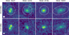 |
Fig. 1. Total intensity maps with contours at 3, 6, 9, and 12× the sky rms. At 18.6 GHz, rms = 1.2, 1.1, 0.6, and 0.7 mJy beam−1 for NGC 3627, NGC 4254, NGC 4736, and NGC 5055, respectively; at 24.6 GHz, rms = 0.7, 0.8, 0.9, and 0.7 mJy beam−1. Photometry apertures and HPBWs are also shown. |
In Fig. 1 we also show the sky apertures used to derive the total flux density Sν. Due to the small size of our maps, the apertures were chosen to be small, but wide enough to enclose all the emission that is deemed to come from the galaxies in both the 18.6 and 24.6 GHz maps. The same apertures were placed on a few positions outside of the targets to estimate the residual background and its fluctuations (see, e.g., Auld et al. 2013; Clark et al. 2018). This procedure gave results consistent with the more traditional sky estimate from an annulus around the source. In Table 2 we give Sν and its uncertainty to which we added, in quadrature, the systematic error discussed in Sect. 2.
Aperture definition and SRT photometry.
In Fig. 2 we show the SEDs of the four galaxies in the 1–30 GHz range, using the SRT photometry and the mid-radio continuum data from T17. Ideally, one should use flux densities obtained by integrating maps over the same aperture at all frequencies. Instead, the flux densities in the compilation of T17 refer to apertures based on the optical size of each galaxy, which are larger than what we used above. Nevertheless, we found that our choice does not significantly alter the estimate of the flux density at SRT frequencies (tests are described in Appendix A.1). We modeled the SED as the sum of three continuum components: (i) synchrotron radiation, dominating in the upper end of the range, which – in the optically thin regime – can be described by a power-law; (ii) free-free emission, which is almost flat with frequency, emerging over synchrotron as the frequency increases; and (iii) AME, which is expected to contribute at the highest frequencies considered here. It is as follows:
 (1)
(1)
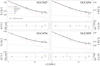 |
Fig. 2. Global SEDs and fits with their uncertainty. We also show each SED component and the T17 fit. Under each SED, we show the residuals Δ=data-model (in percentage of the model). |
where α is the synchrotron spectral index,  and
and  are the amplitudes of the synchrotron and free-free component at 5 GHz, respectively, and the weak frequency dependence of the free-free continuum is taken from Draine (2011). For the AME component, we adopted the spectral template of Battistelli et al. (2019), which was derived by averaging theoretical predictions over a variety of interstellar medium (ISM) environments, using the spdust.2 code (Ali-Haïmoud et al. 2009; Silsbee et al. 2011) and neglecting the most extreme cases presented in Fig. 2 of Dickinson et al. (2018). We scaled the template on its amplitude at 24.6 GHz,
  and, as in Battistelli et al. (2019), we kept its peak fixed (it is located at ν ≈ 25 GHz). We did not include thermal emission from dust, which is negligible in the spectral range we considered (see, e.g., P11).
We fit Eq. (1) to the data using the emcee Python implementation (version 3.0) of the Goodman & Weare’s Affine Invariant Markov chain Monte Carlo (MCMC) Ensemble sampler (Foreman-Mackey et al. 2013). We adopted positive flat priors for α,  ,
,  , and
, and  and obtained their posterior probability distribution function (PDF) by sampling the likelihood function, which is conditional on the data. We used 100 walkers, initially distributed around the T17 fit (assuming negligible AME), and ran a chain of 2 × 10⁴ steps. The PDFs were obtained after deriving the integrated autocorrelation time and neglecting this number of steps a few times so as to remove the burn-in phase from the chain. We tested the convergency of the results by varying the initial conditions (setting higher values for AME), as well as the number of walkers and samples. The fits and uncertainties are shown in Fig. 2, while in Table 3 we present the estimate and uncertainty of each parameter, derived from the median and 0.16 and 0.84 percentiles (see Fig. A.2 for the Bayesian corner plots).
Fit parameters, relative contribution of the various components at 5 and 24.6 GHz, and upper limits for  .
.
The only parameters estimated at high significance are those for the synchrotron component: in particular, our α estimates are consistent within the errors with those of T17. Much more uncertain is the estimate of the free-free component: it is degenerate with that of synchrotron at lower frequencies, contributing to 20–30% of the continuum flux density at 5 GHz (see Table 3); it is also degenerate with the AME component, since the largest contribution to the SED of both emissions insists on the same spectral window for ν ≳ 15 GHz. Because of this, we expected our estimates to be more uncertain than those in T17, which do not include an AME component and use only data with ν ≲ 10 GHz. We compare the results from the two fits in Fig. 3, where we have converted  into the star-formation rate (SFR) since the free-free emission is proportional to the amount of free electrons, and thus to the photoionizing rate (Murphy et al. 2011; T17). Despite the larger uncertainties (but not for NGC 5055), our results are still compatible with T17. Both estimates are also broadly consistent with the SFRs derived by Nersesian et al. (2019) from the analysis of the whole DustPedia UV-to-submm SED, thus independent of the observations in the radio. As shown by Fig. 3, the advantage of deriving the SFR from the radio thermal radiation, in a spectral range unaffected by dust extinction, is compounded by the larger uncertainties due to the fit degeneracies. Data at frequencies above 25 GHz are needed to solve these degeneracies and obtain more precise determinations of SFR from the radio continuum and of the presence of AME.
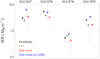 |
Fig. 3. Comparison between SFRs from DustPedia and from |

All three components contribute to the continuum at 24.6 GHz (see Table 3): the synchrotron and free-free fractions are about the same, ∼40%, while the AME fraction is about half that value, ∼20%. However, in no case is the fitted  significant. Thus, in the following discussion, we use upper limits for
  , derived from the 0.95 percentile of the PDF.
Within this work, we also tried to fit the SED without including the AME component in Eq. (1): upper limits on  were then obtained from the residuals between observations and the model (as done in P11). In this case we still obtained plausible fits (not shown) by steepening the synchrotron spectrum and raising the free-free contribution: with respect to fits with AME included,
  values are larger by a factor ∼2 (see the corresponding SFRs in Fig. 3), while the AME upper limits becomes smaller. In fact, as pointed out by P11, this approach might result in a bias toward a lower AME estimate. Nevertheless, either using the
  upper limits from the full fit or those from the residuals to a no-AME fit has no consequence for the rest of the discussion in this work.
4. AME emissivity
In the MW, AME has often been studied in correlation with dust emission at 100 μm (3 THz) (Dickinson et al. 2018). For Galactic latitudes |b|> 10°, PLA16 found  . Usually, the MW estimate has been compared with observations in other galaxies: while in M31 Battistelli et al. (2019) derived a value for
  consistent with the MW, P11 and Tibbs et al. (2018) found smaller ratios for their targets; the same is true for our targets. For simplicity, we used the same notation for the MW (and Magellanic Clouds), where the ratio was derived by correlating surface brightness maps, and for the rest of the galaxies we discuss, where the ratio is between flux densities (equivalent to a ratio between galaxy-averaged surface brightnesses). Also, the ratios were obtained using different radio frequencies: nevertheless, they are not expected to change much in the 20–30 GHz range (by ≲10% for the template of Battistelli et al. 2019). Thus, we neglected any frequency dependence and use, for all objects, the term
  , also when referring to the SRT 24.6 GHz estimates (see Table A.1).
Tibbs et al. (2012) questioned the validity of  as an indicator of the AME emissivity: in fact, the 100 μm flux density – near the peak of dust emission – strongly depends on the grain temperature; instead, under the spinning-grain hypothesis, the low intensity radiation fields responsible for diffuse dust emission have little influence on AME, at least for low density environments (Ali-Haïmoud et al. 2009; Ysard et al. 2011). A better characterization for AME is to derive its emissivity, that is its surface brightness
  normalized to a tracer of the amount of underlying emitting material. Under the assumption that AME is due to dust, we can write
 (2)
(2)
where Σd is the dust mass surface density, B3 THz(Td) is the Planck function for the dust temperature Td, and  is the dust absorption cross-section1. For our targets, temperatures (and dust masses) were obtained from single-temperature modified blackbody (MBB) fits to FIR-submm SEDs by Nersesian et al. (2019), after assuming the average properties of MW diffuse dust from The Heterogeneous dust Evolution Model for Interstellar Solids (THEMIS; Jones et al. 2017): in particular, THEMIS dust is characterized by an effective absorption cross section that can be described by
  /(pc2/M⊙) = 6.9 × 10⁻³ × (ν/3 THz)1.79 (Galliano et al. 2018).
The emissivity  is shown as a function of Td in Fig. 4, where we also included the estimates for the MW and M 31; those for the LMC and SMC (PLA16); and the upper limits for M 33 (Tibbs et al. 2018) and NGC 253, NGC 3034, and NGC 4945 (P11). Seeking uniformity in the estimate of dust parameters, we also performed MBB/THEMIS fits for these objects (Table A.1). Almost all the upper limits are compatible with the estimates in the MW and M 31 and also the LMC and SMC values are not far off. Only for M 33 is
  much lower, suggesting different properties of the ISM and/or the dust grains for this galaxy with respect to the MW and M 31. After computing the spinning-grain emission for the THEMIS dust distribution, most of the spread in Fig. 4 can be reconciled with variations in the ISM density and radiation field intensity (Ysard et al., in prep.).
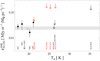 |
Fig. 4.
|


The weighted average of the four determinations is  MJy sr−1 (M⊙ pc−2)−1 (shaded area in Fig. 4). For the dust-to-gas mass ratio of the THEMIS model (0.0074), this converts to 1.4 ± 0.2 × 10⁻¹⁸ Jy sr−1 (H cm−2)−1 (in units of H column density). A possible caveat here can be due to the uncertainties in the determination of the dust column density and to the necessity of using coherent methods for all the objects. For example, if we convert the average emissivity to units of surface brightness per dust optical depth at 850 μm (it is
  ) and express it in temperature (at 22.8 GHz), we obtain 10 ± 2 K, a value close to what PLA16 derived, but for the MW only. The difference might reside in the different reference frequency for estimating the dust surface density, and in the derivation of the dust temperature from the observed SED (using a fixed dust model, in our case, versus a fit of the opacity cross section dependence on the frequency in the Planck analysis, resulting in Td = 19.6 K in PLA16; star in Fig. 4). The fixed power-law expression for
  that we adopted might not be the best choice for describing dust emission when using a single MBB; nevertheless it proved reliable in the estimate of the dust mass (and surface density) under different heating conditions, which is important for the current analysis (see, e.g., Nersesian et al. 2019). Using the average
  , we can estimate
  from S3 THz and the fitted Td (inverting Eq. (2)) or from Md (with Eq. (3)): we derived
  mJy (15 mJy for NGC 5055), which is on the lower side of the spread of Table 3, but still compatible within the large uncertainties from the fit.
In an attempt to understand what makes the detection of AME peculiar in M 31 – where  is estimated to be about 35–70% of the total flux density, while it is a smaller fraction for the rest of the sample – we defined the radio emissivity per dust column density, ϵ1.4 GHz, analogous to
  in Eq. (2) and (3). This quantity is equivalent to dividing S1.4 GHz by the predicted
  if a single
  is valid for all galaxies. In Fig. 5 we plotted ϵ1.4 GHz against the specific SFR, that is the SFR per unit stellar mass, sSFR = SFR/M⋆, which is a physical quantity that shows the largest dichotomy between M 31, at the lowest value, and the rest of the sample. If we do not consider M 33, which apparently has different AME properties, ϵ1.4 GHz for M 31 is almost an order of magnitude smaller than for the other galaxies considered here. Even though more observations (and AME detections) are needed to confirm this apparent trend, one might wonder if AME could be better observed in quiescent spirals in the final stages of their evolution, such as Andromeda, where the build-up of the dust mass has concluded, so that the AME intensity is higher and the radio continuum has a lower luminosity, thus allowing AME to emerge over the other SED components.
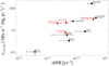 |
Fig. 5. ϵ1.4 GHz vs specific star-formation rate, sSFR. Red symbols are for SRT targets. See Table A.1 for the source of SFRs and M⋆ used to derive sSFR. |
5. Conclusions
We have shown that the upper limits derived for AME in four galaxies observed at SRT (and those for three other objects in the literature) are consistent with the few AME detections, and in particular those for the MW and M 31, once a proper AME emissivity per dust surface density is defined. The analysis presented here is only tentative as it is only based on a few detections. Also, it implicitly relies on the main assumption that AME does not change from object to object, and that its spectrum peaks in between 20 to 30 GHz, as in the diffuse MW medium and in M 31. In the small sample we analyzed, we already found one object, M 33, whose AME emissivity is substantially smaller than those for the other galaxies, possibly on account of a reduced fraction of the small grains responsible for AME (see, e.g., Calapa et al. 2014; Williams et al. 2019). Also, the spinning-grain theory predicts – and some observations in the MW suggest – that the AME spectrum peaks at higher frequency in higher density environments (see, e.g., Dickinson et al. 2018). Thus, different galaxies might have a different AME spectrum depending on the dominant ISM conditions, and on their relative proportion.
Certainly, observations of the full SED beyond 30 GHz and up to the millimeter spectral range could provide further opportunities for new detections and the characterization of AME. Furthermore, they will offer the possibility to solve the degeneracies in the continuum decomposition, without which it will not be possible to fully exploit the use of free-free radiation as a dust-free tracer of the SFR. At the SRT, high frequency observations will become possible soon with the ongoing upgrade to new Q-band (33–50 GHz) and W-band (70–116 GHz) instruments (Govoni et al. 2021).
Equivalently, Eq. (2) can be written as
 (3)
(3)
where Md is the galaxy’s dust mass and D is the distance used for its determination (Eq. (3), as Eq. (2), is eventually independent of D; see also Bianchi et al. 2019).
Acknowledgments
This paper is dedicated to the memory of Jonathan I. Davies, to whom we are grateful, among many other things, for devising the DustPedia and IMEGIN projects. We thank E. S. Battistelli for useful comments and F. Radiconi for sharing with us the AME template used for the M31 analysis. S.B. and V.C. acknowledge support from the INAF main stream 2018 program “Gas-DustPedia: A definitive view of the ISM in the Local Universe”, and from the grant PRIN MIUR 2017 – 20173ML3WW_001. The Sardinia Radio Telescope is funded by the Ministry of University and Research (MIUR), Italian Space Agency (ASI), and the Autonomous Region of Sardinia (RAS) and is operated as National Facility by the National Institute for Astrophysics (INAF). The Enhancement of the Sardinia Radio Telescope (SRT) for the study of the Universe at high radio frequencies is financially supported by the National Operative Program (Programma Operativo Nazionale – PON) of the Italian Ministry of University and Research “Research and Innovation 2014–2020”, Notice D.D. 424 of 28/02/2018 for the granting of funding aimed at strengthening research infrastructures, in implementation of the Action II.1 – Project Proposals PIR01_00010 and CIR01_00010.
References
- Ali-Haïmoud, Y., Hirata, C. M., & Dickinson, C. 2009, MNRAS, 395, 1055 [CrossRef] [Google Scholar]
- Aniano, G., Draine, B. T., Gordon, K. D., & Sandstrom, K. 2011, PASP, 123, 1218 [Google Scholar]
- Auld, R., Bianchi, S., Smith, M. W. L., et al. 2013, MNRAS, 428, 1880 [NASA ADS] [CrossRef] [Google Scholar]
- Battistelli, E. S., Fatigoni, S., Murgia, M., et al. 2019, ApJ, 877, L31 [Google Scholar]
- Bell, A. C., Onaka, T., Galliano, F., et al. 2019, PASJ, 71, 123 [NASA ADS] [Google Scholar]
- Bianchi, S., Casasola, V., Baes, M., et al. 2019, A&A, 631, A102 [NASA ADS] [CrossRef] [EDP Sciences] [Google Scholar]
- Bianchi, S., Murgia, M., Melis, A., et al. 2021, in Proceedings of the International Conference “mm Universe @ NIKA2”, Rome 2021 [Google Scholar]
- Braun, R., Oosterloo, T. A., Morganti, R., Klein, U., & Beck, R. 2007, A&A, 461, 455 [NASA ADS] [CrossRef] [EDP Sciences] [Google Scholar]
- Calapa, M. D., Calzetti, D., Draine, B. T., et al. 2014, ApJ, 784, 130 [NASA ADS] [CrossRef] [Google Scholar]
- Clark, C. J. R., Verstocken, S., Bianchi, S., et al. 2018, A&A, 609, A37 [NASA ADS] [CrossRef] [EDP Sciences] [Google Scholar]
- Clark, C. J. R., Roman-Duval, J. C., Gordon, K. D., Bot, C., & Smith, M. W. L. 2021, ApJ, 921, 35 [CrossRef] [Google Scholar]
- Condon, J. J., Cotton, W. D., Greisen, E. W., et al. 1998, AJ, 115, 1693 [Google Scholar]
- Corbelli, E. 2003, MNRAS, 342, 199 [NASA ADS] [CrossRef] [Google Scholar]
- Dale, D. A., Aniano, G., Engelbracht, C. W., et al. 2012, ApJ, 745, 95 [NASA ADS] [CrossRef] [Google Scholar]
- Davies, J. I., Baes, M., Bianchi, S., et al. 2017, PASP, 129, 044102 [NASA ADS] [CrossRef] [Google Scholar]
- de los Reyes, M. A. C., & Kennicutt, Jr., R. C. 2019, ApJ, 872, 16 [NASA ADS] [CrossRef] [Google Scholar]
- Dickinson, C., Ali-Haïmoud, Y., Barr, A., et al. 2018, New Astron. Rev., 80, 1 [CrossRef] [Google Scholar]
- Draine, B. T. 2011, Physics of the Interstellar and Intergalactic Medium (Princeton University Press) [Google Scholar]
- Draine, B. T., & Lazarian, A. 1998a, ApJ, 494, L19 [NASA ADS] [CrossRef] [Google Scholar]
- Draine, B. T., & Lazarian, A. 1998b, ApJ, 508, 157 [NASA ADS] [CrossRef] [Google Scholar]
- Draine, B. T., & Lazarian, A. 1999, ApJ, 512, 740 [Google Scholar]
- Ejlali, G., Adam, R., Ade, P., et al. 2021, Proceedings of the International Conference “mm Universe @ NIKA2”, Rome 2021 [Google Scholar]
- Emerson, D. T., & Graeve, R. 1988, A&A, 190, 353 [Google Scholar]
- Fatigoni, S., Radiconi, F., Battistelli, E. S., et al. 2021, A&A, 651, A98 [NASA ADS] [CrossRef] [EDP Sciences] [Google Scholar]
- For, B. Q., Staveley-Smith, L., Hurley-Walker, N., et al. 2018, MNRAS, 480, 2743 [NASA ADS] [CrossRef] [Google Scholar]
- Foreman-Mackey, D., Hogg, D. W., Lang, D., & Goodman, J. 2013, PASP, 125, 306 [Google Scholar]
- Galliano, F., Galametz, M., & Jones, A. P. 2018, ARA&A, 56, 673 [Google Scholar]
- Govoni, F., Bolli, P., Buffa, F., et al. 2021, in 2021 XXXIVth General Assembly and Scientific Symposium of the International Union of Radio Science (URSI GASS), 1 [Google Scholar]
- Harper, S. E., Dickinson, C., & Cleary, K. 2015, MNRAS, 453, 3375 [Google Scholar]
- Hensley, B. S., & Draine, B. T. 2021, ApJ, 906, 73 [NASA ADS] [CrossRef] [Google Scholar]
- Hensley, B. S., Draine, B. T., & Meisner, A. M. 2016, ApJ, 827, 45 [CrossRef] [Google Scholar]
- Hoang, T., Vinh, N.-A., & Quynh Lan, N. 2016, ApJ, 824, 18 [NASA ADS] [CrossRef] [Google Scholar]
- Jones, A. P. 2009, A&A, 506, 797 [NASA ADS] [CrossRef] [EDP Sciences] [Google Scholar]
- Jones, A. P., Köhler, M., Ysard, N., Bocchio, M., & Verstraete, L. 2017, A&A, 602, A46 [NASA ADS] [CrossRef] [EDP Sciences] [Google Scholar]
- Katsioli, S., Adam, R., Ade, P., et al. 2021, in Proceedings of the International Conference “mm Universe @ NIKA2”, Rome 2021 [Google Scholar]
- Loi, F., Murgia, M., Vacca, V., et al. 2020, MNRAS, 498, 1628 [NASA ADS] [CrossRef] [Google Scholar]
- Melis, A., Concu, R., Trois, A., et al. 2018, J. Astron. Instrum., 7, 1850004 [NASA ADS] [CrossRef] [Google Scholar]
- Murgia, M., Govoni, F., Carretti, E., et al. 2016, MNRAS, 461, 3516 [Google Scholar]
- Murphy, E. J., Helou, G., Condon, J. J., et al. 2010, ApJ, 709, L108 [NASA ADS] [CrossRef] [Google Scholar]
- Murphy, E. J., Condon, J. J., Schinnerer, E., et al. 2011, ApJ, 737, 67 [Google Scholar]
- Murphy, E. J., Linden, S. T., Dong, D., et al. 2018, ApJ, 862, 20 [NASA ADS] [CrossRef] [Google Scholar]
- Nashimoto, M., Hattori, M., Poidevin, F., & Génova-Santos, R. 2020, ApJ, 900, L40 [NASA ADS] [CrossRef] [Google Scholar]
- Nersesian, A., Xilouris, E. M., Bianchi, S., et al. 2019, A&A, 624, A80 [NASA ADS] [CrossRef] [EDP Sciences] [Google Scholar]
- Orfei, A., Carbonaro, L., Cattani, A., et al. 2010, IEEE Antennas Propag. Mag., 52, 62 [Google Scholar]
- Peel, M. W., Dickinson, C., Davies, R. D., Clements, D. L., & Beswick, R. J. 2011, MNRAS, 416, L99 [NASA ADS] [CrossRef] [Google Scholar]
- Perley, R. A., & Butler, B. J. 2017, ApJS, 230, 7 [NASA ADS] [CrossRef] [Google Scholar]
- Planck Collaboration XVII. 2011, A&A, 536, A17 [NASA ADS] [CrossRef] [EDP Sciences] [Google Scholar]
- Planck Collaboration XXV. 2016, A&A, 594, A25 [NASA ADS] [CrossRef] [EDP Sciences] [Google Scholar]
- Planck Collaboration Int. XV. 2014, A&A, 565, A103 [NASA ADS] [CrossRef] [EDP Sciences] [Google Scholar]
- Planck Collaboration Int. XXV. 2015, A&A, 582, A28 [NASA ADS] [CrossRef] [EDP Sciences] [Google Scholar]
- Prandoni, I., Murgia, M., Tarchi, A., et al. 2017, A&A, 608, A40 [NASA ADS] [CrossRef] [EDP Sciences] [Google Scholar]
- Silsbee, K., Ali-Haïmoud, Y., & Hirata, C. M. 2011, MNRAS, 411, 2750 [NASA ADS] [CrossRef] [Google Scholar]
- Skibba, R. A., Engelbracht, C. W., Aniano, G., et al. 2012, ApJ, 761, 42 [NASA ADS] [CrossRef] [Google Scholar]
- Tabatabaei, F. S., Schinnerer, E., Krause, M., et al. 2017, ApJ, 836, 185 [Google Scholar]
- Tibbs, C. T., Paladini, R., & Dickinson, C. 2012, Adv. Astron., 2012 [CrossRef] [Google Scholar]
- Tibbs, C. T., Israel, F. P., Laureijs, R. J., et al. 2018, MNRAS, 477, 4968 [CrossRef] [Google Scholar]
- Viaene, S., Fritz, J., Baes, M., et al. 2014, A&A, 567, A71 [NASA ADS] [CrossRef] [EDP Sciences] [Google Scholar]
- Viaene, S., Baes, M., Tamm, A., et al. 2017, A&A, 599, A64 [NASA ADS] [CrossRef] [EDP Sciences] [Google Scholar]
- Williams, T. G., Baes, M., De Looze, I., et al. 2019, MNRAS, 487, 2753 [NASA ADS] [CrossRef] [Google Scholar]
- Ysard, N., Miville-Deschênes, M. A., & Verstraete, L. 2010, A&A, 509, L1 [NASA ADS] [CrossRef] [EDP Sciences] [Google Scholar]
- Ysard, N., Juvela, M., & Verstraete, L. 2011, A&A, 535, A89 [NASA ADS] [CrossRef] [EDP Sciences] [Google Scholar]
Appendix A: Additional material
A.1. Tests on aperture photometry
Our apertures are smaller than those used to derive the flux densities in T17, which instead cover the optical size of each galaxy. For example, the 1.36 GHz flux densities listed in T17 were obtained by Braun et al. (2007) using circular apertures with a size of 10 to 15′, almost reaching the whole extent of the SRT maps. Since the original Westerbork Synthesis Radio Telescope images of Braun et al. (2007) are available from the NASA Extragalactic Database (NED), we used them to test the impact of our smaller apertures. We followed the procedure of Dale et al. (2012) to estimate the amount of flux that would go beyond the aperture because of beam smearing. We assumed that the 1.36 GHz image can be used as a higher-resolution proxy for the surface brightness spatial distribution at the SRT frequencies, and smoothed it to the SRT 18.6 GHz resolution, using Gaussian kernels. For each of our targets, the full resolution image is shown in Fig. A.1, with superimposed contours from the smoothed image. We found that the global flux densities of Braun et al. (2007) are larger than those derived by integrating the smoothed maps on our apertures, but only by a moderate factor: 3 to 5% for NGC 3627, NGC 4254, and NGC 4736. The total flux density at 1.36 GHz for NGC 5055 is instead 12% larger. However, this is due, in part, to point sources that are not related to the galaxy (some of which are visible in the southern edge of the map in Fig. A.1): when these are removed, the difference reduces to 5%. Since the errors on SRT photometry are larger, we did not apply any correction. We only note that for NGC 5055, the additional flux density picked from the background sources might also affect the other large-aperture flux densities quoted by T17. Thus, before SED fitting, one should lower those flux densities down by about 7%. Even if this slightly changes the values of the fitted parameters, it has little effect on the general results for this galaxy. Thus, we did not implement this correction either.
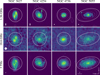 |
Fig. A.1. Maps at different frequencies. Top panels: Westerbork Synthesis Radio Telescope 1.36 GHz images from Braun et al. (2007); the white ellipses show the synthesized beams; the contours show the same maps smoothed to the SRT 18.6 GHz resolution (HPBW = 57″) at surface brightness levels of 0.025, 0.1, 0.25, 0.5, and 0.75 MJy sr−1. Bottom panels: Herschel 3 THz (100 μm) maps from DustPedia, with HPBW = 10″ (white circle); the contours show the maps smoothed to the SRT resolution, at 5, 20, 100, 250, and 500 MJy sr−1. As a reference, the SRT images at 18.6 GHz are shown in the central panel (as in Fig. 1). The apertures adopted in our work are also shown. |
In this work we also made use of DustPedia 3 THz flux densities, obtained by integrating Herschel 100 μm images over apertures matched to contain all emission from the UV to the submm (Clark et al. 2018). We repeated the same exercise on the images from the DustPedia archive: the full resolution maps are shown in the bottom panel of Fig. A.1, with superimposed contours from the same maps smoothed to the SRT resolution (using the convolution kernels of Aniano et al. 2011). This time the flux densities obtained over the larger aperture are almost the same for NGC 3627 and NGC 4736. For NGC 4254 and NGC 5055, instead, the DustPedia flux densities are smaller than those derived on the apertures defined here. Nevertheless, the difference is still compatible with the photometric uncertainties, highlighting the fact that apertures much larger than the apparent size of the objects, though functional in detecting all of the emission, can also result in larger uncertainties due to fluctuations in the sky background and unremoved sources other than the one of interest.
A.2. Details on SED fitting
In Fig. A.2 we show the Bayesian corner plots for the parameters derived from the fit. The figure also shows the marginalized PDF for each parameter together with the median and 0.16 and 0.84 percentiles.
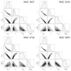 |
Fig. A.2. Corner plots for the parameters describing the SED. Flux densities are in units of jansky (Jy). Marginalized PDFs are shown, the dashed lines marking median values and 0.16 and 0.84 percentiles. |
A.3. Ancillary data
Table A.1 lists the quantities used for producing Fig. 4 and Fig. 5. Besides the upper limits for  for our galaxy sample and the single-T MBB fits to the other targets done in this work, all other data are culled from the literature.
All Tables
Fit parameters, relative contribution of the various components at 5 and 24.6 GHz, and upper limits for .
All Figures
|
Fig. 1. Total intensity maps with contours at 3, 6, 9, and 12× the sky rms. At 18.6 GHz, rms = 1.2, 1.1, 0.6, and 0.7 mJy beam−1 for NGC 3627, NGC 4254, NGC 4736, and NGC 5055, respectively; at 24.6 GHz, rms = 0.7, 0.8, 0.9, and 0.7 mJy beam−1. Photometry apertures and HPBWs are also shown. |
| In the text | |
|
Fig. 2. Global SEDs and fits with their uncertainty. We also show each SED component and the T17 fit. Under each SED, we show the residuals Δ=data-model (in percentage of the model). |
| In the text | |
|
Fig. 3. Comparison between SFRs from DustPedia and from |
| In the text | |
|
Fig. 4.
|
| In the text | |
|
Fig. 5. ϵ1.4 GHz vs specific star-formation rate, sSFR. Red symbols are for SRT targets. See Table A.1 for the source of SFRs and M⋆ used to derive sSFR. |
| In the text | |
|
Fig. A.1. Maps at different frequencies. Top panels: Westerbork Synthesis Radio Telescope 1.36 GHz images from Braun et al. (2007); the white ellipses show the synthesized beams; the contours show the same maps smoothed to the SRT 18.6 GHz resolution (HPBW = 57″) at surface brightness levels of 0.025, 0.1, 0.25, 0.5, and 0.75 MJy sr−1. Bottom panels: Herschel 3 THz (100 μm) maps from DustPedia, with HPBW = 10″ (white circle); the contours show the maps smoothed to the SRT resolution, at 5, 20, 100, 250, and 500 MJy sr−1. As a reference, the SRT images at 18.6 GHz are shown in the central panel (as in Fig. 1). The apertures adopted in our work are also shown. |
| In the text | |
|
Fig. A.2. Corner plots for the parameters describing the SED. Flux densities are in units of jansky (Jy). Marginalized PDFs are shown, the dashed lines marking median values and 0.16 and 0.84 percentiles. |
| In the text | |
Current usage metrics show cumulative count of Article Views (full-text article views including HTML views, PDF and ePub downloads, according to the available data) and Abstracts Views on Vision4Press platform.
Data correspond to usage on the plateform after 2015. The current usage metrics is available 48-96 hours after online publication and is updated daily on week days.
Initial download of the metrics may take a while.