| Issue |
A&A
Volume 658, February 2022
|
|
|---|---|---|
| Article Number | A156 | |
| Number of page(s) | 28 | |
| Section | Planets and planetary systems | |
| DOI | https://doi.org/10.1051/0004-6361/202142378 | |
| Published online | 15 February 2022 | |
Impact of local pressure enhancements on dust concentration in turbulent protoplanetary discs
1
Institute of Astronomy and Astrophysics, Academia Sinica,
Taipei
10617,
Taiwan
e-mail: This email address is being protected from spambots. You need JavaScript enabled to view it.
2
Physics Division, National Center for Theoretical Sciences,
Taipei
10617,
Taiwan
Received:
6
October
2021
Accepted:
7
December
2021
Abstract
The standard core accretion model for planetesimal formation in protoplanetary discs (PPDs) is subject to a number of challenges. One is related to the vertical settling of dust to the disc mid-plane against turbulent stirring. This is particularly relevant in the presence of the vertical shear instability (VSI), a purely hydrodynamic instability applicable to the outer parts of PPDs, which drives moderate turbulence characterized by large-scale vertical motions. We investigate the evolution of dust and gas in the vicinity of local pressure enhancements (pressure bumps) in a PPD with turbulence sustained by the VSI. Our goal is to determine the morphology of dust concentrations and if dust can concentrate sufficiently to reach conditions that can trigger the streaming instability (SI). We performed a suite of global 2D axisymmetric and 3D simulations of dust and gas for a range of values for Σd∕Σg (ratio of dust-to-gas surface mass densities or metallicity), particle Stokes numbers, τ, and pressure bump amplitude, A. Dust feedback onto the gas is included. For the first time, we use global 3D simulations to demonstrate the collection of dust in long-lived vortices induced by the VSI. These vortices, which undergo a slow radial inward drift, are the dusty analogs of large long-lived vortices found in previous dust-free simulations of the VSI. Without a pressure bump and for solar metallicity Z ≈ 0.01 and Stokes numbers τ ~ 10−2, we find that such vortices can reach dust-to-gas density ratios slightly below unity in the discs’ mid-plane, while for Z ≳ 0.05, long-lived vortices are largely absent. In the presence of a pressure bump, for Z ≈ 0.01 and τ ~ 10−2, a dusty vortex forms that reaches dust-to-gas ratios of a few times unity, such that the SI is expected to develop, before it eventually shears out into a turbulent dust ring. At intermediate metallicities, Z ~ 0.03, this occurs for τ ~ 5 × 10⁻³, but with a weaker and more short-lived vortex, while for larger τ, only a turbulent dust ring forms. For Z ≳ 0.03, we find that the dust ring becomes increasingly axisymmetric for increasing τ and dust-to-gas ratios reach order unity for τ ≳ 5 × 10⁻³. Furthermore, the vertical mass flow profile of the disc is strongly affected by dust for Z ≳ 0.03, such that gas is transported inward near the mid-plane and outward at larger heights, which is the reversed situation compared to simulations with zero or small amounts of dust. We find viscous α-values to drop moderately as ~10−3–10−4 for metallicities increasing as Z = 0–0.05. Our results suggest that the VSI can play an active role in the formation of planetesimals through the formation of vortices for plausible values of metallicity and particle size. Also, it may provide a natural explanation for the presence or absence of asymmetries of observed dust rings in PPDs, depending on the background metallicity.
Key words: accretion, accretion disks / hydrodynamics / instabilities / protoplanetary disks / methods: numerical
© ESO 2022
1 Introduction
The standard core accretion scenario for planet formation (Safronov 1972) proposes the growth of micron-sized dust particles until they become planetesimals of a size between 1 km–1000 km that are then subsequently capable of accreting enough solids (Wetherill 1990; Kenyon & Luu 1999) to become terrestrial planets. Furthermore, if they are sufficiently massive, gas accretion is also likely (Mizuno 1980) to become gas giant planets. This scenario is faced with several difficulties. For one, it has been shown that micron-size dust particles hit a so called bouncing barrier when reaching sizes of mms to cms (Blum 2018) upon which further growth due to collisions is hindered. On the other hand, gas drag causes rapid loss of pebbles due to radial drift (Weidenschilling & Cuzzi 1993; Johansen et al. 2014). One possible way to avoid these problems is via a direct self-gravitational collapse of dust grains following their settling to the disc mid-plane (Goldreich & Ward 1973). However, for this to happen, self-gravity must overcome stellar tidal forces as well as collective pressure forces of the dense dust-layer. This, in turn, requires dust-to-gas ratios that are much larger than those typically expected in newly formed protoplanetary discs (Shi & Chiang 2013).
Therefore, processes that can efficiently concentrate dust are actively researched at present. The most popular of these is the streaming instability (SI, Youdin & Goodman 2005; Johansen & Youdin 2007; Youdin & Johansen 2007), a linear dust-gas drag instability. In its original form, which is formulated for an unstratified, monodisperse, and unmagnetized dusty disc, the SI draws energy from the radial dust-gas relative motion. In its nonlinear state, it can lead to strong dust clumping and, hence, contribute to planetesimal formation (Johansen et al. 2009a; Bai & Stone 2010; Simon et al. 2016). However, the strong clumping of pebbles typically requires super-solar values of the vertically-integrated dust-to-gas ratio or metallicity (Johansen et al. 2009a; Bai & Stone 2010; Carrera et al. 2015; Yang et al. 2017; Li & Youdin 2021). It is therefore assumed that additional processes are required to trigger the SI. These processes include particle concentration in zonal flows (Johansen et al. 2009b), pressure bumps (Haghighipour & Boss 2003a,b; Taki et al. 2016; Onishi & Sekiya 2017; Huang et al. 2020), vortices (Barge & Sommeria 1995; Johansen et al. 2004; Klahr & Bodenheimer 2006; Fu et al. 2014; Crnkovic-Rubsamen et al. 2015; Raettig et al. 2015; Miranda et al. 2017; Surville & Mayer 2019), or other instabilities such as dust settling instability (DSI, Squire & Hopkins 2018; Krapp et al. 2020).
In this work, we are particularly interested in dust trapping by pressure bumps and vortices. We are motivated by recent ALMA observations that indicate dust rings – presumably reflective of an underlying pressure bump – are common in bright discs (Andrews et al. 2018; Long et al. 2018); whereas asymmetric dust distributions – possibly reflective of vortices – constitute a smaller, but non-negligible fraction of observed disc morphologies (van der Marel et al. 2021). Carrera et al. (2021a) showed SI can indeed be triggered in the vicinity of a moderate pressure bump embedded in a disc with solar metallicity and cm-sized dust particles, which then leads to planetesimal formation. On the other hand, while dust trapping by vortices has been shown to be efficient, in razor-thin disc simulations, vortices eventually get disrupted due to dust-gas instabilities once the dust-to-gas ratio reaches the order of unity (Fu et al. 2014; Crnkovic-Rubsamen et al. 2015; Raettig et al. 2015; Surville & Mayer 2019). However, Lyra et al. (2018) and Raettig et al. (2021) found that in 3D, vortices do not suffer from destruction because dust feedback is only important in the disc mid-plane, while their vortices are vertically extended. It is also possible to have a combination of pressure bumps and vortices, for example, through the Rossby wave instability (RWI, Lovelace et al. 1999; Li et al. 2001), in the case of which long-lived, dust-trapping vortices do indeed form (Meheut et al. 2012). Understanding the evolution of dust rings and asymmetries has direct application to interpreting observations.
One important element that may influence the aforementioned dust trapping processes is external turbulence. Ever since the discovery of the magneto-rotational-instability (MRI, Balbus & Hawley 1991), accretion in protoplanetary discs was thought to be mediated by MRI turbulent stresses. However, due to low ionization rates in protoplanetary discs, the MRI is most likely extinguished within a region of about ~1–10 AU, known as the “dead zone” (Gammie 1996; Turner & Drake 2009; Armitage 2011; Turner et al. 2014). In fact, recent state-of-the-art magneto-hydrodynamical models show that the inner parts of protoplanetary discs between roughly ~1–20 AU are indeed largely laminar and exhibit angular momentum transport induced by magneto-thermal winds and laminar Maxwell stresses (Gressel et al. 2015; Bai 2015, 2017).
Nonetheless, turbulence in this planet-forming region may still be present owing to the possible occurrence of purely hydrodynamic instabilities. This includes the VSI (Urpin & Brandenburg 1998; Urpin 2003; Nelson et al. 2013; Barker & Latter 2015; Lin & Youdin 2015), requiring a vertically sheared angular velocity profile coupled with rapid cooling of the gas; subcritical baroclinic instability (SBI, Klahr & Bodenheimer 2003; Lesur & Papaloizou 2010; Lyra & Klahr 2011); convective overstability (COS, Klahr & Hubbard 2014; Lyra 2014; Latter 2016), which requires an unstable radial entropy gradient coupled with a local gas cooling time on the order of the orbital time scale; and zombie vortex instability (ZVI, Marcus et al. 2015; Lesur & Latter 2016), which requires slow cooling. A common outcome of these hydrodynamic instabilities is vortex formation, which could seed the SI by accumulating dust, as described above. However, vortex dust trapping has not been simulated explicitly in the case of the VSI and the ZVI, nor has the effect of global disc structures (such as a pressure bump) on any of the above hydrodynamic instabilities.
The aim of this paper is to study the efficiency of dust concentration at pressure bumps and vortices in VSI-turbulent discs. We focus on the VSI because it is a generic phenomenon in the sense that the only structural requirement for it to occur is a radial gradient in temperature or entropy of in principle arbitrary sign, which produces a vertical gradient in the disc’s rotation. Based on models that account for a finite disc cooling time, the VSI is expected to be active at tens of AU (Lin & Youdin 2015). A few studies considered the nonlinear evolution of gas and dust in VSI-turbulent protoplanetary discs by means of global hydrodynamic simulations. Stoll & Kley (2014, 2016) ran 3D simulations with a thermal disc structure governed by stellar irradiation and radiation transport. They found that the VSI is able to generate particle clumps that can, in principle, trigger the SI. Flock et al. (2017) and Flock et al. (2020), employing a similar method, but covering a larger radial domain, (Flock et al. (2020) additionally covering the full 360 degree azimuth, as well as higher resolution, concluded that the VSI is rather an impediment for the early and late phases of planet formation. That is, they found that on the one hand the strong vertical gas motions generated by the VSI effectively lift 0.1–1 mm-sized dust particles such that these are prevented from settling to larger densities at the disc mid-plane. On the other hand, they concluded that accretion of mm-sized pebbles onto planetary embryos in the terrestrial mass range is rendered inefficient by the VSI as the dust-layer thickness likely exceeds the planetary Hill sphere. Picogna et al. (2018) studied the accretion of pebbles with a wide variety of sizes onto planetary cores in a VSI turbulent disc. They found that at ~ 5 AU the fastest growth of protoplanets is achieved for pebbles with τ ~ 1 on account of their fast drift rates. Moreover, they found that the effect of the VSI on this process can be well described through an α-viscosity accompanied by stochastic “kicks” on particles.
However, these studies did not include the dust’s back reaction force onto the gas that arises from their mutual frictional drag. Lin & Youdin (2015) showed that while the VSI is driven by a vertical shear in the gas velocity, it is mitigated by buoyant forces that are usually associated with an adiabatic gas. On the other hand, Lin & Youdin (2017) showed that an isothermal, dusty gas can effectively be described by an imperfectly adiabatic gas for which the finite coupling time between gas and dust as well as global gas temperature gradients act as sources or sinks for the effective entropy of the dust-gas mixture. One important aspect resulting from this model is that the presence of dust leads to an effective buoyancy frequency of the dusty gas, which – under normal conditions – is greater than that of the gas in isolation. Moreover, linear stability calculations of Lin & Youdin (2017) suggest that this dust-induced buoyancy indeed leads to a weakening of the VSI which can promote dust settling. This was confirmed by Lin (2019) with nonlinear axisymmetric hydrodynamic simulations adopting the single fluid model of Lin & Youdin (2017). Furthermore, Lin (2019) showed that dust-to-gas density ratios of a few times the solar value are sufficient to enable efficient settling of particles with Stokes numbers in the range τ ~ 10−3–10−2. However, Lin (2019) did not consider the possible role of pressure bumps and, in addition, their axisymmetric model precludes vortex formation.
In this work, we employ global 2D axisymmetric and non-axisymmetric 3D simulations of a PPD to investigate the conditions under whicha gas pressure bump in a VSI-turbulent disc can raise the local dust-to-gas ratio to such levels that the SI can be triggered to facilitate planetesimal formation. Another question that we aim to answer is whether dust particles will tend to concentrate in vortices or in rings, and whether rings are axisymmetric or not, depending on the disc anddust parameters. Regarding the first point, we show in this work that a moderate pressure bump (A ≳0.2) can collect sufficient amounts of dust to reach order unity dust-to-gas ratios even for solar metallicities Z = 0.01, provided that dust particles have sizes with τ ≳ 10−2. Moreover, we show that the shapes of dust concentrations at a pressure bump become more axisymmetric with increasing metallicity and Stokes number. Generally, a non-axisymmetric appearance of dust rings or the occurrence of vortices requires metallicities of Z ≲ 0.03 in our model.
The paper is structured as follows. In Sect. 2, we describe the basic hydrodynamic equations and the model disc that will be the initial state of our hydrodynamical simulations. There we review basic aspects of dust-gas interaction and the effect of a pressure bump on dust drift. A brief description of the single fluid model of dust and gas, its resulting stability criteria, and the VSI are also provided. This will aid in interpreting the results from our full two-fluid simulations. In Sect. 3, we present and discuss the results of 2D simulations and in Sects. 4 and 5 those of 3D simulations. In Sect. 6, we provide a summary and some conclusions following from our results, as well as prospects for future research.
2 Hydrodynamic disc model
2.1 Basic equations
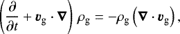
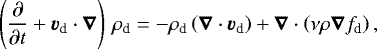
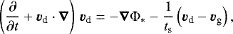
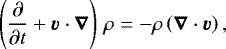
We consider a global hydrodynamic model of a PPD consisting of gas and a single species of dust, governed by the set of dynamical equations:
 (1)
(1)
 (2)
(2)
 (3)
(3)
 (4)
(4)
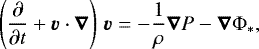
where ρg, ρd, vg and vd are the gas and dust volume mass densities and 3D gas and dust velocities, respectively, in a non-rotating frame with cylindrical coordinates (r, φ, z) and with origin on a central star of mass M* with gravitational potential  , where G is the gravitational constant. The indirect gravitational term, stemming from the fact that the center of mass of the system does not coincide with the center of the star, is ommitted. Furthermore, we neglected self-gravity and magnetic fields. The remaining symbols in the above equations are explained below.
We adopt a locally isothermal equation of state for the gas such that the pressure is:
 (5)
(5)
where the squared sound-speed follows a power-law with constant index − q:
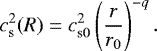 (6)
(6)
The reference sound-speed cs0 = cs(r0), where r0 is a reference radius. Unless otherwise stated, we take q = 1. This value is a bit larger than what is typically expected at large radii in PPDs where the temperature profile is set by stellar irradiation (e.g. Andrews et al. 2009). However, our choice facilitates a comparison with the isothermal simulations by Nelson et al. (2013), Stoll & Kley (2016), and Richard et al. (2016), as well as Manger & Klahr (2018) and Manger et al. (2020), who used the same value. Moreover, it also has the advantage of a radially constant disc aspect ratio such that the required vertical resolution in our simulations is independent of radius. The characteristic gas pressure scale height, Hg = cs∕ΩK, where  is the Keplerian frequency.
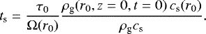
The dust component is treated as a pressureless fluid that interacts with the gas through a friction force (Johansen et al. 2014) quantified by the stopping time1.
 (7)
(7)
where rd and ρd stand for the particle radius and bulk density, respectively. The stopping time is the characteristic timescale for a grain to reach velocity equilibrium with its surrounding gas. The fluid approximation for dust is valid for sufficiently small ts (Jacquet et al. 2011). Typically, we work with the dimensionless Stokes number:
 (8)
(8)
Grains with τ ≪ 1 are tightly (but not necessarily perfectly) coupled to the gas, which either corresponds to small grain sizes or to small distances to the star where the gas density is appreciably higher. The former case is the one that applies to this paper. The Stokes number at r = r0, z = 0, and time t = 0, denoted by τ0, will be a freely specifiable parameter in our model. This means that for a given particle radius and bulk density, its stopping time at a certain location and at a certain time is given by:
 (9)
(9)
We also define

as the dust-to-gas density ratio and the dust fraction, respectively, with the total density ρ = ρg + ρd. We note that fd = ϵ∕(1 + ϵ).
Finally,
![Mathematical equation: \begin{equation*} (((hat{T})))= \rho_{\textrm{g}} \nu \left[ \vec{\nabla} \vec{v}_{\textrm{g}} + \left(\vec{\nabla} \vec{v}_{\textrm{g}} \right) ^{\dagger} - \frac{2}{3} (((hat{U}))) \vec{\nabla} \cdot \vec{v}_{\textrm{g}} \right] \end{equation*}](/articles/aa/full_html/2022/02/aa42378-21/aa42378-21-eq13.png)
is the viscous stress tensor with a (constant) kinematic viscosity, ν, which also describes dust diffusion via the diffusion term in Eq. (3). The symbol † denotes the conjugate transpose and Û stands for the unit tensor. Viscous terms are only included to ensure numerical stability. Hence, ν is chosen to be very small and in derivations which follow below viscous terms are neglected. In particular, ν is much smaller than the typical valueof the α-viscosity (defined in Sect. 2.5) measured in simulations.
2.2 One-fluid model for dust and gas
Our numerical simulations are based on evolving Eqs. (1)–(4) directly (Sect. 2.5). However, as shown byLin & Youdin (2017), many important aspects of dust-gas dynamics can be described within a reduced one-fluid model, governed by the following set of equations:
 (12)
(12)
 (13)
(13)
 (14)
(14)
with density:
the center of mass velocity:
 (15)
(15)
and where the “effective” (dimensionless) entropy of the dust–gas mixture is defined by:
 (16)
(16)
and the effective particle stopping time by:
 (17)
(17)
These equations can be derived from Eqs. (1)–(4) and (5) if dust and gas relative velocities are fixed by the terminal velocity approximation:
 (18)
(18)
which is valid for small particles which are tightly coupled to the gas (Youdin & Goodman 2005). For a more general set of one-fluid equations, see Laibe & Price (2014). We use Eqs. (12)–(14) to motivate the ground state of our disc.
Within this formalism the dust fraction is related to the gas pressure (and temperature) via Eqs. (5) and (11) such that
 (19)
(19)
Similarly, we can define a reduced temperature of the dust-gas mixture
 (20)
(20)
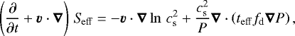
with the gas constant,  and the mean molecular weight μ, such that an increased dust fraction corresponds to a reduced temperature. Furthermore, the flux term (second term on the right hand side of Eq. (14)) stems from the fact that dust drifts into the direction of increasing pressure, as reflected by Eq. (18). Hence, the mixture of a locally isothermal gas with tightly coupled dust behaves as a single-component adiabatic fluid with a non-vanishing energy flux due to the exchange of dust between adjacent fluid parcels and an entropy source term resulting from the imposed global gas temperature profile.
A detailed derivation of this model and applications to various dusty analogs of pure gas instabilities can be found in Lin & Youdin (2017). Here, we merely summarize the important quantities that govern the ground state of our disc and its stability, which can be directly derived from Eqs. (12)–(14). Following Lin (2019), we assume a Gaussian dust-to-gas ratio distribution of
 (21)
(21)
where the gas and dust scale heights are implicitly defined via
 (22)
(22)
This ansatz suggests that ρd follows a Gaussian with scale height, Hd, and ρg follows a Gaussian with scale height, Hg, which is indeed nearly the case as shown below. The initial mid-plane dust-to-gas ratio ϵmid (r) is chosen such that the radial contribution to the effective entropy source vanishes, namely:
 (23)
(23)
to reduce the radial evolution of the initial state (see also Chen & Lin 2018). Of course, in a stratified disc the vertical contribution cannot be zero without diffusion, which results in dust settling (strictly speaking, thus, vz ≠ 0). In practice, we set Hd ≲ Hg such that Hϵ ≫ Hg; that way, the dust is initially well-mixed with the gas. This enables us to define the ground state metallicity as:
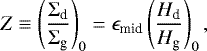 (24)
(24)
with the dust and gas surface mass densities Σd and Σg, respectively. Since Hd ≲ Hg, this also means that ϵmid(r = r0) ≈ Z. In addition to τ0 defined above, Z will also be a used as an adjustable parameter in our simulations. The radial and vertical components of Eq. (13) at equilibrium and under the assumption of axisymmetry are expressed as:
 (25)
(25)
and
 (26)
(26)
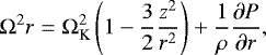
where we defined the orbital frequency Ω = vϕ∕R and applied the thin disc approximation, that is, a Taylor expansion of the gravitational force term in Eq. (13) with respect to the quantity z2∕r2 to next leading order. In addition, we applied the condition that the radial component of v identically vanishes. Furthermore, we neglected the small contribution  due to dust settling2. From Eq. (25), we obtain the orbital frequency
![Mathematical equation: \begin{equation*}\Omega(r,z)= \Omega_{\textrm{K}} \left[1-\frac{3}{2}\frac{z^2}{r^2} -\frac{2 \rho_{\textrm{g}}}{\rho}\eta \right]^{1/2}, \end{equation*}](/articles/aa/full_html/2022/02/aa42378-21/aa42378-21-eq32.png) (27)
(27)
where we define:
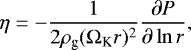 (28)
(28)
which was also defined in Youdin & Goodman (2005). Near the disc mid-plane, we have η > 0 such that the dusty gas rotates with sub-Keplerian frequency. Integration of Eq. (26) using (21) yields the equilibrium gas density profile:
![Mathematical equation: \begin{equation*}\rho_{\textrm{g}} = \rho_{\textrm{g,mid}} \exp\left\{-\frac{z^2}{2 H_{\textrm{g}}^2} -\epsilon_{\textrm{mid}} \frac{H_{\epsilon}^2}{H_{\textrm{g}}^2} \left[1- \exp\left(-\frac{z^2}{2 H_{\epsilon}^2} \right) \right]\right\}. \end{equation*}](/articles/aa/full_html/2022/02/aa42378-21/aa42378-21-eq34.png) (29)
(29)
As expected, for ϵmid → 0 we recover a Gaussian gas density profile with scale height, Hg. In practice, deviations of the gas density from the latter are small, since we consider ϵmid ≪ 1, Hϵ ≫ Hg, and |z| is O(Hg).
We define:
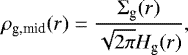 (30)
(30)
such that the vertically integrated gas density yields the surface density Σg (r), which we set to be
 (31)
(31)
with s = 3∕2. The total surface density is Σ = Σg + Σd.
2.3 Dust drift and pressure bumps
Since our aim is to study the effect of a pressure bump on the dust evolution in the disc, we modify the mid-plane density as:
![Mathematical equation: \begin{equation*}\begin{split} \rho_{\textrm{g,mid}}(r) & \to \rho_{\textrm{g,mid}}(r) \times \left[1+ A \exp\left(-\frac{\left(r-r_{0}\right)^2}{2 H_{\textrm{g0}}^2} \right) \right] \\ \quad & = \frac{\Sigma_{0} }{\sqrt{2 \pi} H_{\textrm{g0}}} \left(\frac{r}{r_{0}} \right)^{-p} \left[1+ A \exp\left(-\frac{\left(r-r_{0}\right)^2}{2 H_{\textrm{g0}}^2} \right) \right], \end{split} \end{equation*}](/articles/aa/full_html/2022/02/aa42378-21/aa42378-21-eq37.png) (32)
(32)
with p ≡ s + (3 − q)∕2. That is, we add a Gaussian density bump of amplitude A and width Hg(r0) = Hg0 to the gas mid-plane density profile. While the width of the bump will be kept fixed throughout all simulations, its amplitude A will be varied. Similar density bumps have been employed in numerous previous studies (e.g., Meheut et al. 2012; Taki et al. 2016; Carrera et al. 2021a). With Eq. (32), the equilibrium azimuthal velocity in Eq. (27) is now expressed as:
![Mathematical equation: \begin{equation*}\begin{split} \Omega(r,z) =\;& \Omega_{\textrm{K}} \left\{ 1-\frac{3}{2} \frac{z^2}{r^2} -\frac{\rho_{\textrm{g}} H^2}{\rho r^2} \left[p+q+ r\frac{r-r_{0}}{H_{\textrm{g0}}^2}\vphantom{\frac{A \exp\left(-\frac{\left(r-r_{0}\right)^2}{2 H_{\textrm{g0}}^2} \right)}{1+A \exp\left(-\frac{\left(r-r_{0}\right)^2}{2 H_{\textrm{g0}}^2} \right)}} \right. \right. \\ \quad & \left. \left. \times \frac{A \exp\left(-\frac{\left(r-r_{0}\right)^2}{2 H_{\textrm{g0}}^2} \right)}{1+A \exp\left(-\frac{\left(r-r_{0}\right)^2}{2 H_{\textrm{g0}}^2} \right)} \right] \right\}^{1/2}. \end{split} \end{equation*}](/articles/aa/full_html/2022/02/aa42378-21/aa42378-21-eq38.png) (33)
(33)
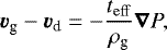
If we restrict our considerations to a narrow region about the mid-plane for the time being, we can neglect vertical gravity and the results of unstratified discs apply. In particular, since our disc is effectively inviscid the ground state planar velocities of dust and gas are those derived by Nakagawa et al. (1986), that is:
![Mathematical equation: \begin{equation*} \vec{v}_{\textrm{d}} = \left[ r \Omega -\frac{1}{2}\frac{\rho_{\textrm{g}}}{\rho} \tau \, v_{\mathrm{drift}} \right] \vec{e_{\varphi}} +v_{\mathrm{drift}} \, \vec{e}_{r}, \end{equation*}](/articles/aa/full_html/2022/02/aa42378-21/aa42378-21-eq39.png) (34)
(34)
![Mathematical equation: \begin{equation*} \vec{v}_{\textrm{g}} = \left[ r \Omega +\frac{1}{2} \frac{\rho_{\textrm{d}}}{\rho} \tau \, v_{\mathrm{drift}} \right] \vec{e_{\varphi}} -\frac{\rho_{\textrm{d}}}{\rho_{\textrm{g}}} v_{\mathrm{drift}} \, \vec{e}_{r}, \end{equation*}](/articles/aa/full_html/2022/02/aa42378-21/aa42378-21-eq40.png) (35)
(35)
where we defined
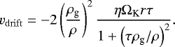 (36)
(36)
These ground-state velocities can be derived from Eqs. (2) and (4) while neglecting vertical stratification. Solutions for α-viscous discs that take into account the vertical disc structure can be found, for instance, in Takeuchi & Lin (2002) and Kanagawa et al. (2017).
The effect of a pressure bump (A > 0) in Eq. (33) has a profound effect on dust drift. This is illustrated in Fig. 1 for different amplitudes A and τ = 10−2. This figure shows how vdrift is essentially controlled by the magnitude of η. Since 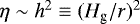 in PPDs (h = Hg∕r being the disc aspect ratio), typical values are η ~ 10−2−10−3. For the most part, η > 0, so dust drifts inwards, but η is non-uniform. The bump thus leads to a sort of “traffic jam" accumulation of dust within a region Δr ~ Hg surrounding the bump center. For the case of A = 0.4, the particle drift comes to a complete halt at a certain radius. This is one reason why pressure bumps in PPDs are expected to serve as the preferred locations for planetesimal formation.
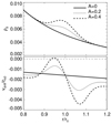 |
Fig. 1 Illustration of the initial mid-plane gas density profile (top panel) according to Eq. (32) and the dust drift velocities (bottom panel) computed from (36) with τ0 = 10−2 for different pressure bump amplitudes A. |
2.4 Disc stability and the VSI
By combining Eqs. (25) and (26), we obtain:
![Mathematical equation: \begin{equation*}\begin{split} r \frac{\partial \Omega^2}{\partial z} = & \frac{c_{\textrm{s}}^2(r)}{\left(1+\epsilon \right)^2} \\ \quad & \times \left[ \frac{\partial \epsilon }{\partial r} \frac{\partial \ln \rho_{\textrm{g}}}{\partial z} -\frac{\partial \epsilon}{\partial z} \frac{\partial \ln P}{\partial r} +\frac{q}{r} \left(1+\epsilon\right) \frac{\partial \ln \rho_{\textrm{g}}}{\partial z} \right]. \end{split} \end{equation*}](/articles/aa/full_html/2022/02/aa42378-21/aa42378-21-eq43.png) (37)
(37)
Hence, the disc’s equilibrium velocity profile is subjected to vertical shear, which constitutes the driving force of the VSI. As pointed out in Lin & Youdin (2017) and Lin (2019), in typical situations, the main source of vertical shear is the disc’s global temperature gradient, quantified through q. However, in regions where sufficiently large gradients of ϵ occur, also the first two terms in the bracket may play a role. We discuss this further below.
Another important quantity for characterizing our disc is the vertical Buoyancy frequency:
 (38)
(38)
which quantifies the stabilizing effect of vertical entropy stratification with respect to adiabatic perturbations. In our vertically isothermal disc this quantity is entirely due to dust-layering. As shown by Lin & Youdin (2017), “dusty” buoyancy mitigates the VSI by stabilizing vertical motions, similarly to classical buoyancy, if  , which is satisfied within sufficiently settled dust-layers. However, in the presence of strong VSI turbulence corrugation of the dust-layer can result in situations where ∂fd∕∂z > 0 for z > 0 and, hence,
  , such that vertical convection may occur.
The occurrence of the VSI in a locally isothermal (dust-free) disc as the one considered here has been established analytically by Nelson et al. (2013), Barker & Latter (2015), and Lin & Youdin (2015). In addition, Nelson et al. (2013) conducted 3D hydrodynamical simulations. Linear stability analyses presented in these papers show that the VSI excites inertial waves that are destabilized by free energy extracted from the disc’s vertical shear. The dominant modes are so called “body modes,” which constitute vertically global (lz ~ hr), radially local (lx ~ h2r), low-frequency (~hΩK) traveling inertial waves that result in either corrugation or “breathing” motion of the disc with respect to the mid-plane. The maximum linear growth rates σ of the body modes in an isothermal disc are governed by the maximum shear in the domain under consideration, namely:
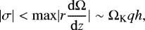
where the latter similarity assumes a domain |z|≲ Hg. This approximation remains applicable even in the presence of dust (Lin & Youdin 2017). However, dust limits the amplitude of turbulent velocity perturbations wherever dust-induced buoyancy becomes significant.
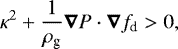
Furthermore, Lin & Youdin (2017) provided the corresponding Solberg–Høiland stability criteria for a dusty gas in the limit of perfect coupling teff = 0 and vanishing radial temperaturegradient q = 0, such that the source terms in Eq. (14) vanish. These criteria are expressed as:
 (39)
(39)
 (40)
(40)
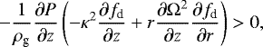
where  is the epicycle frequency squared, and determine the conditions for stability with respect to adiabatic perturbations (Tassoul 1978). These are appropriate since the dust-gas mixture under the aforementioned approximations behaves like an adiabatic gas that conserves the entropy (16). As discussed by Lin & Youdin (2017), the first criterion (39) is expected to be fulfilled in typical situations due to alignment of the two gradients in the second term and since the disc is rotationally supported. The second criterion in Eq. (40) can, in principle, be violated at locations where dust is well mixed vertically but ϵ undergoes sufficiently strong radial variations. Furthermore, if ∂fd∕∂z > 0 occurs for z > 0 the first term in the brackets in Eq. (40) is expected to have a destabilizing effect. We do indeed see that both situations can be realized under certain circumstances in our simulations, which involve strong corrugations of the dust-layer due to the VSI. However, this also means that the VSI is required in first place to violate any of the two criteria in our simulations. We come back to this issue in Sect. 3.2.
Finally, an important instability that is directly involved in the nonlinear saturation of the VSI is the RWI (Lovelace et al. 1999), which can result in the formation of vortices. This instability can be expected when the generalised vortensity, namely:
 (41)
(41)
possesses a local extremum, where  denotes the vertically integrated pressure and where the z-component of vorticity defined in the inertial frame is:
 (42)
(42)
and γ is the adiabatic index. It should be noted that although Eq. (42) and other quantities above are defined using the center of mass velocity in Eq. (15), the latter is nearly equal to both the dust and gas velocities since dust is tightly coupled to the gas in our model. Although the above condition was originally derived for gaseous discs, our locally isothermal gas with tightly coupled dust is equivalent to an adiabatic gas disc with γ = 1 (Lin & Youdin 2017). We therefore expect  to also play a role in our simulations. We note that here, Π arises from the gas only, but Σ accounts for both gas and dust. For brevity, we simply refer to
  as the vortensity.
As outlined in Richard et al. (2016), the VSI generates axisymmetric vortensity rings. These become unstable to the RWI, which consequently leads to the formation of vortices while the vortensity extrema are destroyed (see also Manger & Klahr 2018; Manger et al. 2020). Latter & Papaloizou (2018) argue that in an isothermal disc, where the vertical shear is strictly forced by the imposed global temperature gradient, the amplitude of the VSI-related velocity perturbations is limited by the emergence of Kelvin-Helmholtz parasitic modes that drain energy from the VSI modes and transfer it to smaller scales until viscous dissipation sets in. Based on theoretical arguments Latter & Papaloizou (2018) estimate a maximal turbulent velocity amplitude of saturated VSI modes of a few percent to roughly ten percent of cs. This is indeed in agreement with results from previous isothermal simulations of the VSI and also with the results presented below. The parasitic modes may also result in the formation of small-scale vortices. Moreover, the mid-plane dustlayer can in principle undergo Kelvin-Helmholtz instability (KHI, Johansen et al. 2006; Lee et al. 2010) but this is not expected to be resolved in our simulations. We also note that the pressure bump that is initially placed in our simulations is not expected to be Rossby wave unstable when comparing the values of the width and amplitude used here with those applied in linear stability analyses of Ono et al. (2016) for a Gaussian density bump. That is to say that the largest amplitude bump considered here (A = 0.4) might be marginally unstable to the RWI. However, in our simulations we do not find a qualitative difference between the cases A = 0.2 and A = 0.4.
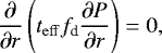
All 2D simulations.
2.5 Hydrodynamic simulations
We solve Eqs. (1)–(4) with the multi-fluid code FARGO3D3 (Benítez-Llambay & Masset 2016; Benítez-Llambay et al. 2019). All quantities are subjected to periodic boundary conditions in azimuth. As for the radial and vertical boundary conditions equilibrium values of gas density and azimuthal velocity are extrapolated into the ghost zones, while gas radial and vertical velocities are set to zero at the boundaries. The only difference for the dust is that densities are subjected to symmetric boundary conditions. Simulations are carried out in spherical coordinates (R, φ, θ). The units are as follows: R0 = Ω0 = G = 1 (R0 equals the radius r0 defined in Sect. 2). We adopt h0 = Hg0∕R0 = 0.05 in all runs. The numerical grid covers 0.5 ≤ R ≤ 1.5, − 3Hg ≤ z ≤ +3Hg, where z = Rtan(π∕2 + θ), and in 3D simulations, 0 ≤ φ ≤ π. The grid resolution of most of our 2D simulations is NR × Nθ = 2160 × 480. Our 3D simulations are conducted on a grid with NR × Nθ × Nφ = 1088 × 256 × 512. This corresponds to a resolution of  . While the radial and vertical resolutions are high compared to previous studies, we adopt a rather moderate azimuthal resolution for reasons of computational resources and since we expect structures to form in our simulations to be predominantly axisymmetric or elongated in azimuthal direction. Selected 2D simulations that are used for a direct comparison with 3D simulations have the same radial and vertical grid cells. The latter are carried out on a GPU cluster which is necessary to cover a substantial domain in parameter space while adopting a reasonable spatial resolution. All simulations are run for 1000 reference orbits. A list of all conducted 2D and 3D simulations with references to the corresponding sections is provided in Tables 1 and 2, respectively.
For analysis of our simulations, we often consider the diagnostic quantities defined as follows. Turbulent vertical momentum transport will be quantified through the Reynolds stress component
 (43)
(43)
where Δvgφ denotes the azimuthal velocity deviation from its ground state value. Averages ⟨ ⟩ are in all cases taken over R, φ (in 3D simulations) and in addition either θ or t. The additional factor sgn(z) is included here in order to facilitate averaging of values above and below the mid-plane z = 0 when presenting its time evolution, which enables a better comparison with the radial stress component defined below. Positive values of  correspond to angular momentum transport away from the mid-plane. Unless otherwise stated, the diagnostic domain of our simulation region is 0.8 ≤ R ≤ 1.2.
In 3D simulations the radial turbulent angular momentum transport is similarly described by
 (44)
(44)
The turbulent α-parameter (Shakura & Sunyaev 1973) is then defined via
 (45)
(45)
Furthermore, the dust scale height, Hd, is computed by fitting a Gaussian along the vertical grid z to the distribution ρd(z).
3 Results of axisymmetric 2D simulations
3.1 Dust settling in the absence of a pressure bump
The settling of dust toward the mid-plane of a VSI-turbulent PPD in the absence of a pressure bump was studied in some detail by Lin (2019), who employed the one-fluid model to describe a dusty gas devised by Lin & Youdin (2017) (Sect. 2.2). Figure 2 illustrates the effect of the particle size, that is, the Stokes number τ0, as well as the background metallicity, Z, on the dust’s ability to settle in the mid-plane of the disc. Shown is the time evolution of (from top to bottom) dust-to-gas scale height ratio, dust-to-gas mid-plane mass-density ratio, rms mid-plane vertical dust velocity, and rms vertically averaged Reynolds stress (as defined in Sect. 2.5), averaged here over the radial domain R0 − H0 < R < R0 + H0. The results in the left panels of Fig. 2, which correspond to a Stokes number of τ0 = 10−3, show a clear systematic trend with increasing metallicity, Z. That is to say that turbulence generated by the VSI is increasingly mitigated with increasing amount of dust in the system. As a result, the latter is ableto settle to a layer of decreasing thickness, which is also reflected in decreased values of the mid-plane vertical dust velocity rms (vdz) and the vertical Reynolds stress parameter  . It can be seen from these curves that the VSI reaches nonlinear saturation after some 100 orbits, in agreement with previous studies (Nelson et al. 2013; Richard et al. 2016; Manger & Klahr 2018). Furthermore, these results agree well with those of Lin (2019), although the impact of dust settling appears to be slightly weaker in our simulations. A substantially weaker trend is seen in the right panel, which shows the effect of an increasing particle size (τ0) for a fixed metallicity Z = 0.01.
In agreement with Lin (2019), the VSI growth rates are largely unaffected by dust. However, there appears to be a weak increase in the early values of rms(vdz) with increasing τ0 and also with increasing Z, the former increase being stronger. Since dust initially settles in such a way that the center of mass velocity vsettle ~ τ0fdcs (at z ~ Hg0), it can be expected that the collective vertical movement of dust and gas toward the mid-plane serves as a seed for VSI modes; these are hence stronger initially for larger τ0 and to a lesser extent for larger ϵ0 [we recall that fd = ϵ∕(1 + ϵ)], explaining the observed trends. Furthermore, since vsettle roughly increases linearly with τ0, dust can consequently settle to a thinner layer before the VSI turbulence develops. In the thinner layer buoyancy (38) is increased so as to stabilize the VSI which reduces stirring of the dust-layer. Outside of the dust layer away from the mid-plane the VSI still drives turbulence, albeit to a weaker extent than in the dust-free case. The effect of particle size observed here is weaker than in the simulations of Lin (2019). Thus, it appears that the overall impact of dust in the system is stronger in the latter study. One reason might be that the single fluid description implicitly assumes the terminal velocity approximation (Youdin & Goodman 2005; Lovascio & Paardekooper 2019) for the dust. Furthermore, the different numerical setup used in Lin (2019) is possibly more dissipative such that the overall level of turbulence is expected to be slightly weaker. Nevertheless, the plots in Fig. 2 demonstrate that the back-reaction force from the dust onto the gas is essential for the weakening of the VSI. The level of turbulent velocity perturbations of a few percent to about 10% in the nonlinear saturation of the VSI is consistent with the theoretical estimates by Latter & Papaloizou (2018).
All 3D simulations.
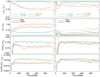 |
Fig. 2 Time evolution of quantities that describe the dust settling process against the emergence of VSI turbulence. From top to bottom these are the ratio of dust-to-gas scale height, the mid-plane dust-to-gas density ratio, the root mean squared mid-plane vertical gas velocity, and the root mean squared (rms) vertical Reynolds stress. The left panels compare different metallicities with fixed τ0 = 10−3, while the right panels compare different Stokes numbers τ0 with Z = 0.01. The dashed red lines in the panels of rms(vgz0) are the exponential |

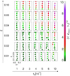 |
Fig. 3 2D simulation survey of the effect of a pressure bump on dust evolution. Shown is the final location of
|
3.2 Dust settling in the presence of a pressure bump
In the following, we investigate the impact of a pressure bump on the accumulation of dust in 2D simulations, which will be compared toresults of 3D simulations in Sect. 4. Figure 3 summarizes a 2D simulation survey for the evolution of dust near a pressure bump over 1000 orbital periods. Results are presented for varying initial amplitude A and for different Stokes numbers, τ0, and ground state metallicities, Z. Each solid circle represents a single simulation in terms of the radial location of the maximal mid-plane dust-to gas ratio  averaged over the last 100 orbits, which in all simulations with A >0 is the result of dust accumulation in the vicinity of the initially imposed pressure bump. The color of each circle represents the value of
  . This figure reveals several noteworthy features. First, in the absence of a pressure bump (A = 0), we find that in order to achieve mid-plane dust-to-gas ratios on the order of unity or greater (and, hence, involving a triggering of the SI and possibly planetesimal formation), a metallicity of at least Z ≈ 0.04 and a Stokes number τ ≳ 0.01 are necessary. On the other hand, for non-vanishing bump amplitude this can be achieved with solar metallicity (Z ~ 0.01) for the same Stokes number.
For lower metallicity (Z = 0.01–0.02) we observe an increasing (radial) inward shift of the radial location of  with increasing τ0 ; whereas for higher metallicity (Z ≳ 0.04), this trend does not exist and
  is in all cases located at R ~ R0. The inward shift at lower metallicities implies that the gas pressure bump has drifted inward while dust is accumulated within its vicinity and migrated along with the gas bump; this is contrary to the cases with higher metallicity, where the pressure bump remains at its origin.
In some cases with lower metallicity and larger bump amplitude (A ≳ 0.3), the resulting dust ring becomes unstable such that it gets disrupted (either partially or entirely) and a new dust ring forms just inside the original one. Thus, in the case of partial disruption two dust rings remain at the end of the simulation, both of which have resulted from the pressure bump. Such simulations are accordingly represented by two filled circles connected by a dotted line in Fig. 3. For large parts of the considered parameter space though, the simulation outcomes show only a subtle dependence on the bump amplitude (as long as it not too small). A similar observation was also reported by Carrera et al. (2021a).
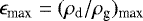
The different outcomes of our simulations are illustrated in Fig. 4 which displays the time evolution of ϵ (we plot its fourth root for improved visibility) for three simulations with Z = 0.01, Z = 0.03 and Z = 0.05 (in all cases A = 0.4), respectively. The over-plotted profiles illustrate the gas pressure at different times which are indicated by horizontal dashed lines. Since our simulations are locally isothermal, these curves effectively correspond to the evolution of the gas density. The arrows indicate dust drift velocities as computed from (36), which, as expected describe the movement of dusty “clumps” quite well. Interestingly, particle feedback seems to enhance the gas pressure bump for lower background metallicities, rendering the pressure bump unstable such that it eventually disrupts. In principle, such an enhanced pressure bump could potentially be subjected to the RWI (Ono et al. 2016) which, however, is suppressed due to the imposed axisymmetry in these simulations. Disruption of the dust ring occurs much earlier for the case with intermediate metallicity Z = 0.03. Whether the dust ring in the case Z = 0.01 would disrupt in our simulation ultimately depends on the radial size of the domain since sufficient dust needs to be accumulated before the region outside the ring gets depleted of dust. On the other hand, no instability appears to occur for the case with Z = 0.05. These findings are primarily confirmed in full 3D simulations, as presented in Sect. 4.
3.3 Instability of dusty rings
It turns out that the drifting, as well as the splitting of dust rings, are both the result of a violation of at least one of the Solberg–Høiland criteria for a dusty gas (Eqs. (39), (40)). In regions of low metallicity, the VSI is sufficiently vigorous to strongly puff up the dust-layer such that dust adjacent to a high-density ring possesses a substantially greater scale height than the former, such that a relatively strong radial gradient |∂fd∕∂R|≫ 0 can occur away from the mid-plane and at the same time a small vertical gradient ∂fd ∕∂z ≈ 0. If ∂fd ∕∂R ≪ ∕ ≫ 0, accommodated by a vertical shear around the mid-plane ∂Ω2∕∂z > ∕ < 0, this results in a violation of (40).
VSI turbulence can also result in situations4 where ∂fd∕∂z > 0 for z > 0, which, along with κ2 > 0 leads to a violation of (40) provided ∂fd∕∂R ≈ 0. Such situations are realized for instance within the dust “bubble" directly inside the dust ring in the simulation with Z = 0.03. Moreover, a positive ∂fd ∕∂z above the mid-plane translates to vertical convection since then  [Eq. (38)].
Furthermore, in low-metallicity regions, the VSI modes, when attaining sufficiently large amplitude, can directly violate the Rayleigh criterion such that Eq. (39) is violated since the first term on the right hand side of Eq. (39) dominates the second term practically everywhere in our simulated discs. In certain parts of such a region, we also find (40) to be violated where ∂fd∕∂z < 0 for z > 0, which is expected near the mid-plane. The dominance of the first term over the second in (39) is due to the system still being rotationally supported, so that the buoyancy term ∇P ⋅∇fd is small in comparison. Radial profiles of κ2 appear noisy on the grid level and they vary in time. It is not unexpected that κ2 can drop to negative values. The VSI operates on small radial length scales and the linear modes are also nonlinear solutions, at least in the incompressible limit (Latter & Papaloizou 2018). Therefore, we can assume that linear VSI modes are capable of growing to high amplitudes. Specifically the vertical component of vorticity, which amounts to κ2 ∕2Ω in axisymmetric models. Therefore, this quantity can grow until the Rayleigh criterion is violated. In 3D simulations, however, linear modes will undergo KHI or RWI and the flow develops non-axisymmetry before the Rayleigh criterion is actually violated.
Figure 5 illustrates the unstable behavior of dust rings in the same simulations as those shown in Fig. 4. The upper panels display the dust-to-gas ratios for a time near 450 orbits, which is just prior to the dust ring in the simulation with Z = 0.03 being disrupted atthe expense of a new dust ring, which subsequently drifts inward. This is also when the dust ring in the simulation with Z = 0.01 starts to drift inward. The remaining panels from top to bottom are the two time-averaged (over the range 350-450 orbits) Solberg–Høiland expressions, namely, ⟨SH1⟩, ⟨SH2⟩, corresponding to Eqs. (39) and (40), and the rms averaged Reynolds stress  , corresponding to Eq. (43). What these plots mainly show is that the Solberg–Høiland criteria are violated in various places, mostly away from the mid-plane. However, both stability criteria are most severely violated in the puffed up dust-layers adjacent to the dust ring of each simulation. In the unstable regions just inside of the dust rings for the cases Z = 0.01 and Z = 0.03 we find a substantially increased Reynolds stress Rθφ and, hence, an increased vertical angular momentum transport (away from the mid-plane). We expect this to be responsible for the inward drift or disruption of the dust rings in these simulations.
 |
Fig. 4 Time evolution of the dust-to-gas ratio in the vicinity of a pressure bump with amplitude A = 0.4. Compared from left to right are different metallicities Z = 0.01, 0.03, 0.05 with the same τ0 = 4 × 10⁻³. The over-plotted solid curves are the mid-plane gas pressure at times indicated by horizontal dashed lines. The dashed curves are the initial gas pressure for comparison. The arrows indicate the direction of dust movement as predicted by Eq. (36) and are all normalized to have the same length. |
3.4 Discussion
Previous works investigating the evolution of dust in the vicinity of a pressure bump (Taki et al. 2016; Onishi & Sekiya 2017; Huang et al. 2020; Carrera et al. 2021a) have not reported any unstable behavior on the part of dust rings that formed at a pressure bump, as described in the previous sections. Although Taki et al. (2016) found that the pressure bump gets destroyed by the particle feedback within hundreds of orbital periods without sufficient reforcing, this turned out to be caused by the neglect of vertical stellar gravity and, hence, dust sedimentation in the mid-plane (Onishi & Sekiya 2017). Also, for the parameters used by Taki et al. (2016) (Z = 0.1, τ0 = 1) or Huang et al. (2020) (Z = 0.05, τ0 ~ 0.25), we do not expect drifting or disruption in our simulations to occur as well, based on Fig. 3.
Huang et al. (2020) found an instability of dust rings with dust-to-gas ratios of order unity, but their simulations were in 2D (vertically integrated) and, thus, omitting the vertical disc stratification as well. Furthermore, the instability found by Huang et al. (2020) does, in principle, only require a dust ring with sufficiently sharp edges and a dust-to-gas ratio on the order of unity, such that gas within the dust ring is forced to attain Keplerian velocity; these authors speculate that the edges of the ring could be unstable to the RWI due to a sharp drop of the vorticity ωz, which is not captured in our 2D axisymmetric simulations. Also, our finding that the simulation with Z = 0.05 does not show unstable behaviour despite having developed a dense sharp dust ring would thus be hard to explain.
We have verified that neither drifting nor disruption of dust rings occurs in 1D radial simulations or 2D vertically unstratified, axisymmetric simulations. Furthermore, we ran simulations with reduced temperature gradient (i.e., smaller values of |q|) and found that the unstable behavior diminishes, with the dust rings behaving essentially laminar, with decreasing |q|. These findings, which are presented in Appendix A, support our picture of a dusty gas instability that is triggered by the VSI turbulent motions and which lead to the phenomena described above. Indeed, the VSI does not occur in an unstratified disc as there is no vertical shear. Also a reduction of |q| weakens the vertical shear and, hence, the VSI.
 |
Fig. 5 Meridional cuts of (from top to bottom) the dust-to-gas ratio at 450 orbits, the averaged Solberg–Høiland expressions (39), (40) (the left hand side terms) and root mean squared vertical Reynolds stress. Averages are taken over the time 350–450 orbits. In the panels ⟨SH1 ⟩ and ⟨SH2⟩, negative values are indicated by a black color. These plots compare the same simulations as in Fig. 4 and illustrate the emergence of a dusty gas instability through a violation of the Solberg–Høiland criteria. |
4 Results of 3D simulations: Turbulent properties and dust rings
In this section, we present the results of 3D simulations where the main focus lies on the collection of dust into rings or vortices (discussed in Sects. 4.2 and 5, respectively). Before turning to these topics, we first present a brief investigation of the turbulent properties of the dusty gas disc. Where possible, we draw comparisons with our 2D simulations.
4.1 Turbulent flow properties
We start by comparing the strength of VSI turbulence as it occurs in 3D and 2D simulations without an initial pressure bump. Figure 6 shows the time evolution of the spatially averaged vertical Reynolds stress (43), which represents a running time-average to smooth out strong fluctuations (upper panels), as well as its time-averaged vertical profile (lower panels). Time averages have in the lower panel been taken over the last 400 orbits. Overall, turbulence takes comparable magnitudes in 2D and 3D simulations. The influence of dust on the strength of turbulence appears to be complicated. At low metallicity and a small Stokes number, the presence of dust appears to result in additional stirring of the gas such that the stress  is enhanced as compared to the dust free case. This applies to both 2D and 3D simulations, although the effect is stronger in 2D. We conjecture that this increased turbulent activity in the low metallicity and Stokes number cases shares its origin with the dusty gas instability discussed in Sect. 3.3. This is illustrated in Fig. 7, where the plots correspond to 900 orbits. In the plots of the dust-to-gas ratios, small-scale vortices are visible along the edges of the strongly corrugated dust-layers in the lower metallicity case. The second row displays, similarly as in Fig. 5 the time-averaged (900–1000 orbits) expression ⟨SH2⟩, corresponding to (40). The third row represents the time-average of the gas-vorticity component
  . The last two rows show the radial and vertical gradients of the dust fraction fd. This figure underlines that increased vorticity production stems mainly from radial structuring and to a smaller extent from vertical structuring of the dust-layer, which we verified by inspection of the two terms within the brackets on the right hand side of (40). This structuring of the dust-layer is caused by corrugation (an idea first put forward by Lorén-Aguilar & Bate 2015). In principle, since there are locations where ∂fd ∕∂z > 0 for z > 0 – and hence
  – the condition for vertical convection is locally fulfilled at these locations at some time. It is unclear if the latter has a notable influence on the disc turbulence. The figure also shows how the vertical gradient ∂fd ∕∂z has a strongly stabilizing effect in the case Z = 0.05 that overcompensates for the potentially destabilizing effects of the radial gradient ∂fd ∕∂R. Thus, at a greater metallicity, dust sufficiently weakens the VSI such that dust can settle onto a thinner and denser layer that is less prone to corrugation motions. This leads to a strongly reduced production of vorticity, ωφ, around the mid-plane. Subsequently, the Reynolds stresses fall below the dust-free values. In principle an increased vorticity could also be due to KHI as adjacent dusty gas layers shear past each other in the vertical direction due to corrugation. However, if KHI were the reason for the observed increased vorticity and Reynolds stress we would expect this effect to be strongest in the dust-free case since the KHI does not rely on the presence of dust and the VSI is causing the corrugation which would be the origin of the KHI. The observed strong increase in Rθφ when adding small amounts of dust would not be expected in this scenario. Also the finding that the Solberg–Høiland criteria are actually violated in the corrugated dusty layer points to the dusty gas instability for being the origin of the increased hydrodynamic activity. Moreover, our resolution is likely not sufficiently high to resolve such parasitic KHI modes (C. Cui, priv. comm.).
Interestingly, Lorén-Aguilar & Bate (2015), who conducted smoothed particle hydrodynamics simulations of a PPD with very similar setup (3D, locally isothermal) found a similar corrugation of the mid-plane dust-layer. However, they concluded this to be the result of a baroclinic instability that arises in response to a violation of Eq. (40), which they defined for a pure gas with an entropy  – in contrast to our definition expressed via Eq. (16), which is also that of Lin & Youdin (2017) and where ρg is replaced by the total density ρ. This subtle difference in the definition of S leads to a change of sign in the criterion for the onset of vertical convection, namely, ∂fd ∕∂z > 0 for z > 0 in contrast to Eq. (7) of Lorén-Aguilar & Bate (2015). From the results presented in Fig. 7, we conclude that the criterion adopted here is adequate since the settled dust-layer itself is stable, whereas regions above and below it are marginally unstable. Corrugation of the dust-layer in our simulations is a direct result of velocity perturbations of VSI modes and it is the corrugation that facilitates the conditions for a violation the second Solberg–Høiland criterion or a locally unstable vertical entropy stratification. Furthermore, it remains questionable that the VSI did not develop in the simulations of Lorén-Aguilar & Bate (2015) despite the required physical conditions being fulfilled.
To further illustrate the impact of dust on the turbulent properties of the disc, we compare in Fig. 8 the vertical dependence of the time and radially and azimuthally averaged radial mass flow and radial velocity of gas and dust in 2D and 3D simulations, respectively. At low metallicity (lower panels in all cases), we recover the results of Stoll & Kley (2016) and Manger & Klahr (2018), namely, that gas flows inward near the disc’s mid-plane; whereas at larger heights, it flows outward. A similar flow pattern is also found in our 2D simulations, which is, nonetheless, of a slightly different magnitude that may in some cases exceedthe 3D values. The observation that inflow velocities near the mid-plane for low metallicities in 2D and 3D simulations take comparable values most likely stems from the anisotropic (Reynolds) stress generated by the VSI and that the most prominent perturbations excited by the VSI are vertically global modes of relatively short radial wavelength ≲ Hg. This anisotropy was studied by Stoll et al. (2017), who attempted to model the turbulent accretion flow induced by the VSI in 3D simulations by a laminar viscous accretion flow in 2D axisymmetric simulations and found that the vertical viscosity coefficient (characterizing  ) in their models needed to be 650 times larger than the radial component (characterizing
  ) in order to set the vertical structure of the accretion flow pattern in the two simulations in agreement. In passing, we note that we obtained a total gas accretion rate of ~−1.2 × 10⁻⁵ Σg0ΩK for the dust-free 3D simulation by vertically integrating the mass flow profile shown in the bottom left panel of Fig. 8. This value seems consistent with the value ~ − 2.4 × 10⁻⁵ Σg0ΩK reported byManger & Klahr (2018), who adopted a larger disc aspect ratio of h = 0.1. However, a quantitative study of accretion rates requires carefully defined boundary conditions and is not be considered here.
Many aspects of the profiles plotted in Fig. 8 can be understood by considering basic aspects of dust-gas drag (Sect. 2.3). Considering the 3D results for the time being, for small Stokes numbers τ0 = 10−3 dust and gas averaged velocities are essentially equivalent, regardless of Z, which is also in agreement with results in Fig. 17 of Stoll et al. (2017). For larger τ0, dust velocities become increasingly negative and gas velocities increasingly positive, which is also expected. Moreover, In the dense dusty mid-plane layer that forms in simulations with higher values of τ0 and Z, radial drift velocities become small as ρd > ρg. However, with increasing metallicity and Stokes numbers the gas and dust radial velocity profiles change substantially. For instance, for Z = 0.1 and τ0 = 10−3 (and actually even for Z = 0.05, which, however, is not shown here) or for Z = 0.03 and τ0 = 5 × 10⁻³ – the profiles have changed in such a way that material is flowing inward away from the mid-plane while it flows outward in narrow regions close to the mid-plane. Interestingly this flow profile resembles to some extent the standard laminar isotropic α-viscosity case (e.g., Takeuchi & Lin 2002). The reason for this change is due to different VSI modes being dominant in the different cases. This is illustrated for the examples Z = 0.01, 0.1 with τ0 = 10−3 in Fig. 9 and can also be seen in the vertical profiles of the Reynolds stress for these parameters in Fig. 6. At low metallicity and for increasing Stokes number, we find that the radial mass fluxes qualitatively agree with those of Stoll & Kley (2016) (their Fig. 18). Departures occur for the radial dust velocities at larger Stokes numbers, where they found that the radial dust velocity away from the mid-plane is always directed outward and larger in magnitude than the radial gas velocities. In contrast, we find that the dust velocities become negative for larger Stokes numbers, as mentioned above. These discrepancies with Stoll & Kley (2016)are most likely due to the neglect of particle feedback in their simulations. Moreover, they added particles at a time atwhich the VSI had reached a quasi-steady state whereas we simulate both dust and gas coevally. However, the overall qualitative agreement between 2D and 3D simulations lends additional credibility to our results. Comparing averaged velocities with averaged mass fluxes for the gas is generally straight forward. The gas is nearly incompressible such that its averaged mass flow is essentially the averaged gas velocity multiplied with the initial Gaussian density profile. This does not, however, apply to the dust whose mid-plane density can exhibit complex time variations owing to corrugation. A detailed analysis of the dust mass flow profiles is beyond the scope of this paper.
Figure 10 compares the dust settling process in 2D and 3D simulations with metallicities Z = 0.01–0.1 and Stokesnumbers τ = 10−3–10−2. Shown are the dust-to-gas scale height ratio and the mid-plane dust-to-gas density ratio. Overall, the results agree quite well. For both the 2D and 3D simulations, the averages are taken within a radial domain of 0.8 ≤ R ≤ 1.2. For the 3D simulations an additional averaging over azimuth has been performed. Apart from the smallest metallicity and Stokes number cases, dust settling is somewhat stronger in 2D simulations, which is expected from the results in Fig. 6. All simulations shown were run with the same radial and vertical resolution and domain sizes. For the 3D simulation with Z = 0.01 and τ = 10−2, the disc region under consideration already becomes significantly depleted of dust by the end of the simulation. This is in part due to vortices that form and collect inward drifting dust and eventually leave the considered disc region. This will be discussed in more detail in Sect. 5.
Furthermore, Fig. 11 illustrates the effect of dust on the VSI’s ability to transport angular momentum in radial direction in 3D simulations. Shown is the time evolution, which again is in the form of a running time average, as well as time-averaged vertical profiles of the α-viscosity parameter (45). The averages are taken in the same fashion as in Fig. 6. In contrast to the behavior of  (Fig. 6) which describes vertical angular momentum transport, α decreases steadily with increasing metallicity, even at low metallicity. The reason is that the main driver of an increased
  is corrugation of the dust-layer which can only occur in vertical direction. The values α ≲10−3 extracted from our dust-free reference simulation are in good agreement with those of Nelson et al. (2013), but almost a factor 10 larger than those reported by Manger et al. (2020) for the same disc aspect ratio h = 0.05. Several other studies report smaller values (Stoll & Kley 2016; Pfeil & Klahr 2021; Flock et al. 2020), mainly due to their adoption of a more realistic equation of state, improved by at least a finite cooling time (compared to the isothermal approximation), which is known to mitigate the VSI (Lin & Youdin 2015). The most likely reason for the difference to the values of Manger et al. (2020) is the higher radial and vertical grid resolution adopted in our simulations. Furthermore, Manger et al. (2020) found that the resolution in azimuthal direction has a subdominant effect on the VSI activity, in contrary to the strong dependence on the azimuthal domain size (Manger & Klahr 2018).
 |
Fig. 6 Comparison of the vertical Reynolds stress (43) in 2D and 3D simulations for different metallicities, Z, and Stokes numbers, τ0. Upper panels: running time-averages (spatially averaged over the entire diagnostic domain 0.8 ≤ R ≤ 1.2), while the lower panels display the time-averaged (over the last 400 orbits) vertical profiles. The dashed curve is in all panels for 2D and 3D the same, respectively. The horizontal dotted line indicates “zero”, such that positive and negative values correspond to angular momentum transport away from the mid-plane and towards the mid-pane, respectively. |
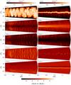 |
Fig. 7 Illustration of the origin of the increased vertical Reynolds stress |

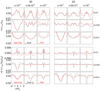 |
Fig. 8 Vertical profiles of the averaged radial dust and gas velocities (upper three rows) and the dust and gas mass flows (lower three rows) in 3D (left panels) and 2D (right panels) simulations. The Stokes number τ0 increases from left to right while Z increases from the lower to upper panels. For comparison, in the panels corresponding to Z = 0.01 and τ0 = 10−3 we additionally plot the result of a dust-free simulation. Averages have been taken over the last 400 orbits and over 0.8 ≤ R ≤ 1.2. The dust mass flows are additionally scaled with a factor 1∕ϵ0 as compared to the gas mass flows. The horizontal axis displays − 2Hg ≤ z ≤ 2Hg in all panels. |
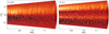 |
Fig. 9 Meridional plots of the time-averaged Reynolds stress |


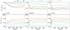 |
Fig. 10 Comparison of the dust settling process in 2D and 3D simulations for different metallicities Z and Stokes numbers τ0. Shown are the ratios of the dust and gas scale heights (upper panels) and the mid-plane dust and gas densities. All quantities are averaged in radius and in 3D simulations also in φ. |
4.2 Dust rings
One class of prominent substructures in PPDs that ALMA has revealed in recent years are rings and gaps, visible in the dust mm continuum or spectral line emission (e.g., van der Marel et al. 2013, 2021; ALMA Partnership 2015; Andrews 2020). A fraction of the well-observed dust rings exhibit more or less strong (typically crescent shaped) non-axisymmetries whose origin is still topic of debate. One generally assumes that there are two main mechanisms which can generate these structures. These are so-called “horseshoes,” which constitute non-axisymmetric gas enhancements in discs just outside the inner cavity that has been cleared by a stellar binary (Ragusa et al. 2017) or vortices generated at a pressure bump adjacent to a gap that is assumed to be created by a planet of sufficiently high mass (e.g., Zhu & Stone 2014). The latter mechanism is the one that is specifically relevant to this work and here we wish to investigate whether (and under what conditions) dust rings that form at a pressure bump in an VSI turbulent disc can attain dust to gas ratios that could result in planetesimal formation and, second, whether dust rings can be subjected to any persistent non-axisymmetries.
Figures 12–15 show dust rings that formed in 3D simulations in response to an initially seeded pressure bump, for different background metallicities Z, Stokes numbers (τ0 = 0.001 and τ0 = 0.01) and bump amplitudes (A = 0.2 and A = 0.4), respectively. The dotted and dashed curves illustrate the azimuthally averaged final and initial gas pressure profile, respectively. We verified by means of test simulations that the pressure bumps in these simulations are not subject to the RWI5. It should be kept in mind that our resolution is not sufficient to resolve small-scale instabilities such as the SI, which may disrupt the dust rings, although the SI might be less efficient in a turbulent disc. That being said, what Figs. 12–15 reveal is that an increase of the parameters Z and τ0 (and to some extent also A) results in a transition from a preference to form dusty vortices toward a preference to form dusty rings. Generally speaking, we find an increasing axisymmetry of formed dust enhancements when increasing these parameters. We hypothesize that the reason for this transition is the same as that for the increased stability of dust rings found in our 2D simulations when increasing the same parameters, since essentially this weakens the VSI. When comparing the results presented in this section with those of our 2D simulations which are summarized in Fig. 3, we find many similarities. For instance, the cases with the smallest Stokes number τ0 = 10−3 and lower metallicity Z ≲ 0.03 are lacking any notable dust enhancements at the pressure bump site, although we observe the formation of weak dusty vortices in 3D. Furthermore, in Sect. 3.2 we discussed the occurrence of a dusty gas instability and how it results in disruption or inward drift of dust rings. The parameter regime within which this happens can be directly determined from Fig. 3. Indeed, Figs. 12–15 show that also in 3D simulations dust rings undergo inward drift and the magnitude of this drift is larger for larger (smaller) Stokes number (metallicity). For the purposes of illustration, Fig. 16 compares the radial locations of dust rings as observed in 2D and 3D simulations for two metallicities (Z = 0.01, 0.03) and bump amplitudes (A = 0.2, 0.4) and Stokes number τ0 = 10−2. For the case Z = 0.01, dust rings in 2D simulations (dashed curves) drift slightly faster than in 3D simulations (solid curves), whereas the opposite is the case for Z = 0.03. The behavior for Z = 0.01 can be explained considering that the dusty gas instability which causes the inward drift is somewhat stronger in 2D than in 3D (cf. Fig. 6). On the other hand, the negligible inward drift in the 2D simulations with Z = 0.03 is a consequence of the much larger value of ϵ attained in the corresponding dust rings (cf. Fig. 3). For the same reason (i.e., increased ϵ) drift speeds for the cases with A =0.4 are generally smaller than for the corresponding cases with A = 0.2. That being said, drift speeds of dust rings according to Fig. 16 can get as fast as ~ 0.2Hg0/(100 orbits) in 3D simulations and ~0.3Hg0/(100 orbits) in 2D simulations.
Moreover, the dust rings formed in simulations with Z ≤ 0.03 are subject to strong turbulent distortions, whereas those corresponding to larger Z are nearly axisymmetric. In the former cases, the gas pressure bump is dragged along with the dust ring and in some cases even amplified, similar as in corresponding 2D simulations (Fig. 4). Also one can clearly see strong corrugation of the dust-layer adjacent to the ring for these cases in the upper panels which show meridional contour plots. This corrugation facilitates the dusty gas instability discussed in Sect. 3.3.
One difference is that in 3D simulations instability leads to vortex formation, which is suppressed in 2D axisymmetric simulations. An example for the evolution of an unstable dust ring in a 3D simulation is presented in Fig. 17. In this case the dust ring continuously produces new vortices that split off and drift inward. The driving force of this unstable behavior is, similarly to the 2D simulations, the VSI. The attained dust-to-gas density ratios in 3D dust rings are not nearly as high as in 2D, which is due to planar turbulent diffusion generated by the VSI and quantified through α (as discussed in Sect. 4.1) in 3D simulations.
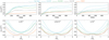 |
Fig. 11 α-viscosity parameter (45) as measured in 3D simulations for different metallicities and Stokes numbers. The dotted curves correspond to a dust-free simulation. The upper panels display the running time-average of the spatially averaged value while the lower panels show vertical profiles, averaged in time. |
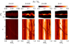 |
Fig. 12 Snap shots of dust-to-gas density ratio at late times (800−1000 orbits) in simulations including a pressure bump with amplitude A = 0.2 and with Stokes number τ0 = 10−3. The dashed and dotted curves represent the initial and final mid-plane gas pressure profiles, respectively. |
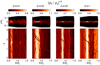 |
Fig. 13 Snap shots of dust-to-gas density ratio at late times (800−1000 orbits) in simulations including a pressure bump with amplitude A = 0.2 and with Stokes number τ0 = 10−2. The dashed and dotted curves represent the initial and final mid-plane gas pressure profiles, respectively. |
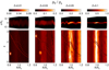 |
Fig. 14 Snap shots of dust-to-gas density ratio at late times (800−1000 orbits) in simulations including a pressure bump with amplitude A = 0.4 and with Stokes number τ0 = 10−3. The dashed and dotted curves represent the initial and final mid-plane gas pressure profiles, respectively. |
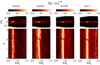 |
Fig. 15 Snap shots of dust-to-gas density ratio at late times (800–1000 orbits) in simulations including a pressure bump with amplitude A = 0.4 and with Stokes number τ0 = 10−2. The dashed and dotted curves represent the initial and final mid-plane gas pressure profiles, respectively. |
5 Results of 3D simulations: Vortices
In this section, we discuss the appearance of vortices in 3D simulations and their capability to concentrate dust and hence assist in planetesimal formation.
5.1 Dust-free simulations
Figure 18 shows the mid-plane vorticity (42) after around 600 reference orbits in 3D dust-free simulations with an initially seeded pressure bump of varying amplitude A. The lower-left panel corresponds to the run presented in the lower left frame of Fig. 8 in Manger et al. (2020) and we find good agreement between the sizes ΔR ~ Hg0 and aspect ratios RΔφ∕ΔR ~ 8–10 of the largest vortices appearing in these simulations. Moreover, the size of these vortices appears to increase with increasing bump amplitude A. They appear after ~ 200–400 orbits, where earlier times correspond to larger values of A. Numerous small-scale vortices are present as well. These are short-lived and cannot be tracked in our simulations since our time resolution is ~ 50 orbits. Similarly small vortices have been found in other studies (Richard et al. 2016; Manger & Klahr 2018) and their survival times were estimated to be several orbits. Although it is not entirely clear if the correspondence between vortex size and bump amplitude isphysical or a coincidental outcome of our simulations, a possible explanation is that large vortices grow by absorption of small-scale vortices and that this can happen more efficiently in the vicinity of a pressure bump. Paardekooper et al. (2010) have shown that in razor-thin disc models, vortices undergo migration by emitting sound waves inwards andoutwards in an asymmetrical fashion that is similar (but not identical) to planets embedded in a disc. The direction of migration is related to the background surface density gradient, such that vortices migrate toward regions of larger surface density. This should also imply migration towards the mild pressure maximum corresponding to a large vortex. However, since the small-scale vortices have a small vertical extent of considerably less than one scale height (Richard et al. 2016), the vertically-averaged results of Paardekooper et al. (2010) potentially do not apply to these vortices. It is therefore not clear whether or not they can migrate over any significant distance and be absorbed by a large vortex before they dissipate. On the other hand, the migration and also merging of larger vortices is directly observed in our simulations – similarly to what was reported by Manger et al. (2020).
Figure 19 shows the time evolution of the radial gas density profile (azimuthally averaged) at the mid-plane for the same simulations as in Fig. 18. The dashed vertical lines indicate the radial location of the large vortex for the three latest times. In all simulations the vortex survives for hundreds of orbits and migrates inwards. This is in agreement with the results reported by Manger & Klahr (2018), Manger et al. (2020) and also Pfeil & Klahr (2021). In addition, the density bump smears out through turbulent diffusion and redistribution of mass within the disc in response to the (turbulent) angular momentum transport generated by the VSI, an aspect recently considered by Manger et al. (2021). Indeed, we find a pileup of mass around R ~ 0.6R0 (outside the diagnostic domain) in a similar manner as shown in Fig. 9 (bottom left panel) of Manger et al. (2021).
Apart from the size of the vortices, the results in Fig. 19 do not provide evidence that the pressure bump has an effect on migration of large vortices or that it is a preferred location for the formation of the latter, since the vortex in the simulation with A = 0 forms at a very similar radius as in all other simulations with A > 0. Nevertheless, we hypothesize that large vortices result from merging of smaller vortices and that this is more likely to occur if vortex radial migration is mitigated. The latter is expected to depend on the surface density gradient (Paardekooper et al. 2010) and we therefore expect a more efficient growth of vortices at a pressure bump. To further test this hypothesis we ran additional simulations with different surface density slopes s (and hence different mid-plane gas density slopes p). The results of these simulations, which are presented in Appendix B, show that a flatter mid-plane density profile leads to slower migration speeds and larger vortices and support our hypothesis.
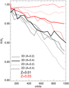 |
Fig. 16 Radial locations of dust rings in 3D (solid curves) and 2D (dashed curves) simulations for metallicities Z = 0.01 (black curves), and Z = 0.03 (red curves) and bump amplitudes A = 0.2 (thin curves)and A = 0.4 (thick curves). The locations correspond to the maximum value of ϵ at each time. The sporadic reversals of the drift direction are due to turbulent fluctuations of the dust density within the rings. The 3D simulations are the same as in Figs. 13 and 15. The 2D simulations are those shownin Fig. 3. |
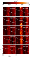 |
Fig. 17 Time evolution of an unstable dust ring in a 3D simulation with parameters τ0 = 4 × 10⁻³, Z = 0.03, and A = 0.4. The dashed and solid curves are the initial and current mid-plane gas pressure profile, respectively. One can clearly see an amplification of the gas pressure bump and unstable behavior of the dust ring, as it develops strong non-axisymmetries and splits ofa vortex which subsequently migrates inward. |
5.2 Dusty simulations without a pressure bump
Our dusty 3D simulations reveal that large (ΔR ~ Hg0) vortices collect dust and survive for typically hundreds of orbital periods, which is similar to the survival time of pure gas vortices discussed above. Within a simulation time of 1000 reference orbits, we find large, long-lived vortices only for metallicities Z ≲ 0.03 and – if Z = 0.03 – only for small Stokes numbers τ0 ~ 10−3. We generally do not observe larger, long-lived vortices in simulations with Z ≥ 0.05. The exception is in a simulation with Z = 0.05 and τ0 = 10−3, where at late simulation times past 1000 orbits we find the formation of a large vortex, but its dust content is negligible compared to ambient turbulent dust lanes that are present in the simulation region as well. We attribute the absence of long-lived vortices at high metallicities and Stokes numbers to the corresponding weakening of the VSI by dust feedback and its ability to form vortices. Therefore, we also expect weaker vortensity perturbations in simulations with larger Z, which is illustrated in Fig. 20, where the vortensity  is given by Eq. (42).
None of the vortices that formed in our simulations without an initial pressure bump attained dust-to-gas ratios of unity or greater. The largest value we find is ϵ ~ 0.7 in a vortex by the end of the simulation with Z = 0.01 and τ0 = 10−2. This is in strong contrast to the values of ϵ attained in vortices that formed in the 3D shearing box simulations of the COS by Raettig et al. (2021), where even for an initial value of Z ~ 10−4, vortices formed rapidly and after tens of orbits values of ϵ ~ 10 were reached within the vortices. The main reason for these differences is certainly the much weaker vertical turbulent velocities generated by the COS (~10–100 times smaller than for the VSI) and perhaps to some extent the larger Stokes numbers τ0 ≥ 5 × 10⁻² considered in that work. That being said, we cannot rule out that larger dust-to-gas ratios could be obtained with Stokes numbers > 10−2, a larger radial domain, or both; the latter of which would supply more dust for trapping. (An inflow outer boundary condition would have the same effect.) Because of dust drift, we can already find significant dust depletion in the diagnostic domain 0.8 ≤ R ≤ 1.2 by the end of the aforementioned simulation with τ0 = 10−2, such that the collection of dust in the vortex is already hampered. This effect will be even more severe in simulations with larger Stokes numbers such that these would either require a substantially larger radial domain size or inflow of dust at the outer boundary.
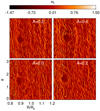 |
Fig. 18 Mid-plane plots of the z-component of the gas vorticity Eq. (42) after 540 orbits in dust-free simulations with an initial pressure bump of varying amplitude A. |
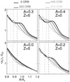 |
Fig. 19 Evolution of the mid-plane gas density for dust-free simulations with an initial pressure bump of varying amplitude A. The dashed lines indicate the location of the large vortex in these simulations at the three latest times. |
5.3 Dusty simulations including a pressure bump
In the presence of dust, the evolution of a pressure bump can differ significantly from the dust-free evolution discussed in Sect. 5.1, which is illustrated in Fig. 21. In Sect. 4.2, we show that pressure bumps give rise to the formation of dust rings, vortices, or a combination of both. While pressure bumps are expected to either trap dust or cause “traffic jams” to produce dust rings (see Sect. 2.3), the frequent formation of vortices at the pressurebump is less obvious based on above dust-free results in Sect. 5.1 (we recall that our initial pressure bumps are stable against the vortex-forming RWI.) However, in Sect. 3.3 we found that dust rings at low and intermediate metallicities are locations of increased hydrodynamic activity due to violations ofone of the Solberg–Høiland criteria (Eqs. (39)–(40)), which are associated with corrugationsof the dust-layer by the VSI. In 3D, we can therefore expect such dust rings to be preferred locations for the formation of vortices, for a given range of dust-parameters. Similarly to the 2D simulations shown in Fig. 4, such unstable dust rings also go along with an increased gas density such that the pressure bump is effectively being amplified, which is clearly seen in the lower right and upper left panel of Fig. 21. Within this scenario, it is also consistent that no vortices form at dust rings in simulations with sufficiently large Z ≳ 0.05, due to effective weakening of the VSI by dusty buoyancy. This can clearly be seen when comparing Fig. 5 with Fig. 14.
Examples of dusty vortices that form at a pressure bump are found in Figs. 14, 17, and below. The latter figure also demonstrates that dust is more settled in the vortex core, which is clearly seen in the contour plot of scale height ratio, Hd ∕Hg. Unlike bump-free simulations, for moderate initial pressure bumps (A = 0.2–0.4), we do find vortices that collect sufficient amounts of dust such that the SI should be triggered within these if it were to be resolved. Figure 22 illustrates the evolution of large, long-lived vortices that form at a pressure bump with an amplitude A =0.46 in simulations with metallicity Z = 0.01 and Stokes numbers τ0 = 10−3 and τ0 = 10−2, respectively.These vortices survive a considerable time span of about 500 orbits. For τ0 = 10−3, the vortex core does not attain unity dust-to-gas ratios within the simulation timescale and steadily migrates inward with a rate of ~ 0.4Hg0/(100 orbits), comparable to that of dust-free vortices (cf. Appendix B), until it eventually dissolves in the background flow.
On the other hand, the vortex formed in the simulation with τ0 = 10−2 reaches a dust-to-gas ratio that is at unity at about 200 orbits following its formation and a maximum value of almost 4 after 400 orbits. Therefore, it can be expected that the SI would be triggered with higher grid resolutions. Due to the larger dust-to-gas ratio the inward drift of the vortex is substantially slower in this case. Furthermore, the shape of the dust distribution within the vortex is more elongated in the case of larger Stokes number (or equivalently,larger particle size). By the end of the simulation the vortex dissolves into a turbulent, non-axisymmetric circumferential dust ring. A similar trend in the distribution of dust particles of different sizes in vortices was reported by Crnkovic-Rubsamen et al. (2015) and Surville & Mayer (2019) for vortices in 2D shearing sheet simulations.
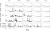 |
Fig. 20 Radial profiles (azimuthally averaged) of the vortensity (41) at different times in simulations with Stokes number τ0 = 10−3 and different metallicities Z. The occurrence of sharp peaks in this quantity suggests that the smallest scale structures appearing in our simulations are most likely not sufficiently resolved in order to properly compute numerical derivatives contained in the quantity
|

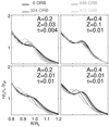 |
Fig. 21 Evolution of the mid-plane gas density in dusty simulations with different metallicity Z, Stokes number τ0 and pressurebump amplitude A. |
5.4 Discussion
The small-scale, compact vortices found in our simulations and those of Richard et al. (2016) and Manger et al. (2020) are assumed to be the result of parasitic KHI that inflict the VSI modes, thereby controlling their nonlinear saturation amplitudes (Latter & Papaloizou 2018). The rapid dissipation of these vortices is likely caused by the elliptic instability (Lesur & Papaloizou 2009; Railton & Papaloizou 2014), which is more vigorous for small vortex aspect-ratios. Larger vortices with aspect ratios of around 5 or larger do not fit in the scenario just described. First of all, their properties are different from the vortices that were described in Latter & Papaloizou (2018). For instance, the large scale vortices found here are vertically extended structures where the vorticity perturbation extends over more than one gas scale height, which is illustrated in Fig. 23. Moreover, these elongated vortices are likely less affected by the elliptic instability in our simulations since for such vortices this instability grows slowly and requires high radial resolution.
Richard et al. (2016) found that long-lived vortices with larger aspect ratios can form in their simulations if the disc possesses relatively long cooling times ≳0.5Ω−1 and steep temperature profiles with q = 2. They argued that for such disc parameters, the SBI (Petersen et al. 2007a,b; Lesur & Papaloizou 2010) can amplify the vortices, whereas the SBI is inactive for shorter cooling times (such as our locally isothermal discs), shallower temperature profiles, or both. However, since the VSI most likely appears in disc regions that are not expected to fulfill the criteria for the SBI (although the simulations of Pfeil & Klahr (2021) suggest that the VSI can exist in the inner, optically thick part of a PPD, where also the SBI is expected to be active) Richard et al. (2016) concluded that the vortices resulting from the VSI are unlikely to promote planetesimal formation on global scales. It was later shown by Manger & Klahr (2018) that the VSI can generate large, long-lived vortices in an isothermal disc and that the reason for the absence of such vortices in the simulations of Richard et al. (2016) was an azimuthal simulation domain that was simply too small.
Furthermore, it is unlikely that the mechanism that eventually destroys the large-scale vortices in our simulations is the same as that in previous 2D simulations of dusty vortices (Fu et al. 2014; Crnkovic-Rubsamen et al. 2015; Raettig et al. 2015; Surville & Mayer 2019), which might be the heavy core instability (Chang & Oishi 2010). The results presented in Fig. 22 suggest, rather, that the lifetime of the large scale vortices in our simulations is independent of the amount of dust concentrated within them. It can be expected that whatever instability attacked vortices in the aforementioned high-resolution shearing sheet simulations is not resolved here. Since the vortices do disappear on timescales that are in agreement with the lifetimes of dust-free vortices (discussed in Sect. 5.1), this suggests that the mechanism of destruction is also the same. Most likely this is a combination of turbulent diffusion and Keplerian shear that disrupts large vortices in our simulations. The influence of the elliptical instability (Lesur & Papaloizou 2009), the parasitic KHI (Latter & Papaloizou 2018), or the VSI itself in the vortex core must be clarified in future high-resolution 3D simulations.
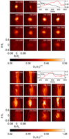 |
Fig. 22 Example evolution of large dusty vortices that formed at a pressure bump (A = 0.4) in 3D simulations with metallicity Z = 0.01 and Stokes numbers τ0 = 10−3 (upper panels) and τ0 = 10−2 (lower panels). The contour plots show the dust-to-gas ratio. The insert plot displays the vortex location (black curve) and its maximum dust-to-gas ratio (red curve) as functions of time. |
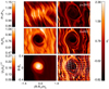 |
Fig. 23 Detailed view of the large dusty vortex corresponding to the upper panels of Fig. 22. Snapshots of the dust-to-gas ratio (lower left panel), the dust-to-gas scale height ratio (middle left panel) and the mid-plane gas pressure scaled with its azimuthally averaged value at each radius are shown. The right panels show the dust vorticity (42) at different heights (z = 0 in the lowerright panel). The arrows in the lower right panel illustrate the dust velocity in the frame co-moving with the Keplerian shear and where in addition the spatial average of the azimuthal velocity over the displayed region has been subtracted to suppress the contribution of the vortex bulk motion. |
6 Summary and conclusion
We studied the effect of a pressure bump on the evolution of dust in a PPD with fully developed turbulence generated by the VSI. We conducted global 2D axisymmetric and 3D, locally isothermal simulations of gas and dust, modelling the outer parts (R ≳ 10 au) of PPDs that are heated by stellar irradiation. Dust particles were treated as a pressureless fluid and its back reaction onto gas through drag was taken into account. In particular, we investigated the influence of the particle’s Stokes number τ0, the disc’s initial dust abundance Z = Σd∕Σg, and the amplitude A of the pressure bump on dust accumulation at the bump site. In our models, A corresponds to the fractional increase in the gas surface density over a bump width of two gas scale heights compared to the ambient background. The range of considered Stokes numbers τ0 = 10−3−10−2 corresponds to particle sizes from ~280 μm at 10 au to ~9 μm at 100 au for τ0 = 10−3 or between ~3 mm and 90 μm for τ0 = 10−2.
The VSI is a robust, purely hydrodynamical instability in PPDs that drives weak to moderate turbulence and transport in PPD dead zones (Nelson et al. 2013; Stoll & Kley 2014, 2016; Manger et al. 2021). We find α-viscosity parameter values ~ 10−4–10−3, where lower values correspond to larger Z. These α values are consistent with those reported in the aforementioned studies. VSI activity weakens with dust-loading because of stabilizationprovided by dust-induced buoyancy (Lin 2019).
When active, the VSI results in strong vertical mixing of dust particles and is therefore a suitable source of turbulence to test the robustness of planetesimal formation in the vicinity of a pressure bump (Flock et al. 2017; Lin 2019; Flock et al. 2020). We find that a moderate pressure bump A ≳0.2 collects sufficient amounts of dust to reach local dust-to-gas density ratios ϵ > 1 at solar metallicity, Z = 0.01, and Stokes numbers, τ0 ~ 10−2.
We find a morphology of dust concentrations at the pressure bump transition from non-axisymmetric to axisymmetric with increasing background metallicity Z or Stokes number τ0. In particular, at lower Z ≲ 0.01–0.03 and τ0 ~ 10−3, a weak dust ring forms that gives rise to the formation of one or more vortices with enhanced (but still much lower than unity) dust-to-gas ratio. These vortices subsequently migrate inwards until they leave the computational domain or dissolve in the background flow. In these simulations, the pressure bump decays due to turbulent diffusion. At low metallicities and larger Stokes numbers, τ0 ≳ 5 × 10⁻³, dust rings of significant dust-to-gas ratios (order unity) form that are generally highly turbulent, non-axisymmetric in appearance, and undergo inward drift. In some cases, such as the one shown in the lower panel of Fig. 22, these rings spawn a vortex that concentrates most of the dust within the ring before it shears out into a new dust ring after some hundreds of orbits. Moreover, in certain parameter regimes (intermediate values of τ0 and larger A = 0.4) such dust rings can spawn multiple vortices, which either split off and migrate inward, or, as described above, concentrate most of the dust within the ring throughout the entire simulation time (cf. Fig. 17). In such simulations, the pressure bump remains intact or even gets significantly amplified. The behavior of dust rings just described can be explained by the presence of an instability of dusty rings that is fed by gradients in the dust-to-gas ratio that arise from the corrugation motion of the dust-layer adjacent to the ring due to the VSI.
At large metallicities Z ≳ 0.05, we find no notable long-lived vortices form. Instead, high density dust rings with weak or negligible non-axisymmetries develop, with dust-to-gas ratios that exceed unity by a large margin for Stokes numbers τ0 ≳ 5 × 10⁻³.
Our 2D axisymmetric simulations capture large parts of the findings described above. That is, they adequately describe the settling of dust in the disc mid-plane as well as the formation of dust rings at pressure bumps. These dust rings can undergo inward drift and disruption due to a dusty gas instability powered by the VSI. Moreover, critical combinations of Z and τ0 required to surpass unity dust-to-gas ratios agree fairly well with those inferred from 3D simulations. For example, in the absence of a pressure bump, Z ≳ 0.05 is required to achieve this for τ0 ≳ 10−2, while in the presence of a mild pressure bump (A ≳ 0.2), a solar metallicity Z ≳ 0.01 is sufficient. On the other hand, the formation of dust-collecting vortices and other possible non-axisymmetric structures are obviously not captured in axisymmetric simulations. Also, due to the lack of turbulent planar (α) diffusion in the latter simulations dust rings can become very thin at large Z values with dust-to-gas ratios much higher than in 3D simulations.
Our results are potentially relevant to the small (albeit non-negligible) fraction of asymmetric dust distributions compared to axisymmetric ones, as seen in ALMA images of PPDs (van der Marel et al. 2021). From our results, it may be possible to infer the background metallicities or particle sizes in observed PPDs that contain dust rings based on the degree of asymmetry. As we have shown, asymmetries in dust rings “naturally” occur in a VSI-turbulent disc when the metallicity in the region where a pressure bump starts to accumulate dust is sufficiently low (Z ≲ 0.03). A direct triggering of the RWI is not required in this scenario.
Our findings do support the idea that vortices are a possible explanation for observed asymmetries of dust rings in PPDs – as was recentlydebated in van der Marel et al. (2021), since it is possible (given reasonable dust parameters) for new vortices to continuously be formed in unstable dust rings, such as the one presented in Fig. 17. Moreover, our results indicate that vortices formed by the VSI at a pressure bump of moderate amplitude A =0.2–0.4 could, underthe right circumstances, play a role in planetesimal formation, since order unity dust-to-gas ratios can be achieved within them for small particle sizes τ ~ 10−2 and solar metallicity Z = 0.01.
In this study, we did not consider the possibility of a reforcing mechanism for the pressure bump, such as in Carrera et al. (2021a) and Carrera et al. (2021b). Based on our finding that dust rings, which form at a pressure bump, drift inwards for lower metallicities Z ≲ 0.03 (Sect. 4.2), we speculate that a single pressure bump, if it were reinforced, could (in principle) spawn multiple dust rings that would end up at smaller disc radii. As long as dust keeps flowing in from larger radii, we would expect a continuous cycle in which the pressure bump collects dust into a ring and, as soon as the dust-to-gas ratio reaches a certain (low) level, instabilities (as discussed in Sect. 3.2) set in and the dust ring will drift inward. Verifying this scenario would require either a considerably larger domain size or a continuous inflow of dust at the outer domain boundary. Furthermore, the inward drift of dust rings (cf. Fig. 16) may be important when inferring the locations of bump-generating structures such as planet gaps or snow lines; that is to say that the observed dust rings may not be formed in situ.
The spatial resolution of our simulations is insufficient to resolve several small-scale instabilities that can affect the evolution of dusty rings and vortices. In particular, we did not resolve the SI (Youdin & Goodman 2005), which will start playing a role when unity dust-to-gas density ratios are attained. Previous 2D simulations (Fu et al. 2014; Raettig et al. 2015; Crnkovic-Rubsamen et al. 2015; Surville & Mayer 2019) suggest that vortices are destroyed by small-scale dust-gas instabilities once dust-to-gas ratios (and, hence, dust feedback) become sufficiently high. On the other hand, the 3D shearing box simulations by Lyra et al. (2018) and Raettig et al. (2021) show that vertically extended vortices can remain intact even when high values of ϵ are reached, as feedback is only important at the mid-plane. In 3D, however, the elliptical instability (Lesur & Papaloizou 2009) should operate but is most likely unresolved in our models, which may shorten the lifetime of the large vortices seen in our simulations. Other effects, such as the dust settling instability (Squire & Hopkins 2018; Krapp et al. 2020), the KHI of the mid-plane dust-layer (Chiang 2008; Barranco 2009), and vertically shearing streaming instabilities (Ishitsu et al. 2009; Lin 2021) are also not captured. Conducting global 3D simulations of the VSI that also resolve the SI and these small-scale instabilities are computationally too expensive at this time. Schäfer et al. (2020) performed global 2D axisymmetric simulations of the VSI and the SI and this setup could be used as a first step to investigate some aspects of the common effect of the SI and VSI on dust rings.
For a realistic modelling of dust concentration in rings and vortices, we would ultimately need to consider simulations that employ a distribution of particle sizes that are (in addition) allowed to change due coagulation and fragmentation, since particle growth is expected to be enhanced in these structures. Even in the absence of the latter, the presence of multiple dust species can have a significant impact on the evolution of the SI (Bai & Stone 2010; Krapp et al. 2019; Paardekooper et al. 2020; Zhu & Yang 2021; Schaffer et al. 2021) – this, in turn, can affect the evolution of dust rings and dust-laden vortices.
Throughout this study, we assume a fixed temperature profile with power-law index q = 1. Decreasing this value will result in a weakening of the VSI, which is then much more sensitive to dusty buoyancy (Lin 2019), shifting critical values of the metallicity Z encountered in our study to lower values. The opposite will be true if q is increased. Eventually, a more realistic equation of state including a finite cooling time should be considered. For instance, Fung & Ono (2021) showed in 2D shearing sheet simulations that a finite cooling time can have adverse effects on vortex life times at disc radii that are relevant to our work. On the other hand, the dust-free simulations of Richard et al. (2016) and Pfeil & Klahr (2021) suggest that large long-lived vortices can be supported by the SBI (Lesur & Papaloizou 2010) when the cooling time is increased. In a follow-up work, we will explore the impact of finite cooling times and multiple grain sizes on the evolution of pressure bumps in turbulent PPDs.
Acknowledgements
We thank the anonymous reviewer for their insightful report and C. Cui for useful discussions. This research is supported by the Ministry of Science and Technology of Taiwan (grants 107-2112-M-001-043-MY3, 110-2112-M-001-034-, 110-2124-M-002-012) and an Academia Sinica Career Development Award (AS-CDA-110-M06). Simulations were conducted at the TIARA High-Performance Computing cluster and the TAIWANIA cluster hosted by the National Center for High-performance Computing (NCHC).
Appendix A Influence of temperature slope q on dusty gas instability
In Section 3.3, we describe how the VSI leads to the emergence of a dusty gas instability by inducing a corrugation motion of the dusty mid-plane layer. To further substantiate this hypothesis, we additionally conducted 2D axisymmetric simulations, including an initial pressure bump with A =0.4 and with reduced values of the temperature slope, q, as this should result in a weaker VSI and hence a weaker dusty gas instability. The results of these simulations are presented in Figures A.1 and A.2 for the cases τ0 = 6 ⋅ 10−3 with z = 0.01 and z = 0.03, respectively. From left to right, the simulations adopt a temperature slope q = 1 (the fiducial value), q = 0.75, q = 0.5, and q = 0.1. According to observational studies (Andrews et al. 2009), the two intermediate values q = 0.75 and q = 0.5 should be the most realistic ones to model the outer parts of PPDs. With decreasing value of q, we find that the inward drifting motion as well as the splitting of dust rings is increasingly mitigated. However, the inward drift remains significant for all but the smallest value of q considered here. The simulations with the smallest value q = 0.1 are almost entirely laminar with only very weak VSI activity. Additional unstratified 2D simulations, as well as 1D simulations with various values of q ≤ 1 that we carried out, are very similar to the cases with q = 0.1 shown here and therefore, we do not present them here.
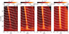 |
Fig. A.1 Time evolution of the dust-to-gas ratio in the vicinity of a pressure bump with amplitude A = 0.4. Compared from left to right are different temperature slopes q, with the same metallicity Z = 0.01 and Stokes number τ0 = 6 ⋅ 10−3. The over-plotted solid curves are the mid-plane gas pressure at times indicated by horizontal dashed lines. The dashed curves are the initial gas pressure for comparison. The arrows indicate the direction of dust movement as predicted by Equation (36) and are all normalized to have the same length. |
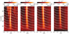 |
Fig. A.2 Time evolution of the dust-to-gas ratio in the vicinity of a pressure bump with amplitude A = 0.4. Compared from left to right are different temperature slopes q, with the same metallicity Z = 0.03 and Stokes number τ0 = 6 ⋅ 10−3. The over-plotted solid curves are the mid-plane gas pressure at times indicated by horizontal dashed lines. The dashed curves are the initial gas pressure for comparison. The arrows indicate the direction of dust movement as predicted by Equation (36) and are all normalized to have the same length. |
Appendix B Influence of density slope p on vortex evolution
As described in Section 5.1, we hypothesize that the size of large vortices depends on their capability to absorb small vortices in their vicinity. Based on the study of Paardekooper et al. (2010) we expect this capability to be increased for flatter surface density profiles where small vortices are expected to be more efficiently attracted by the mild pressure maximum corresponding to a large vortex (cf. Figure 23). To test this hypothesis, we conducted 3D dust-free simulations with varying gas surface mass density slope, s (and, hence, varying mid-plane gas density slope, p). These simulations are presented in Figure B.1. The results in the left panels correspond to ~ 1000 orbits and illustrate that for |p|≤ 1 vortices are substantially stronger and more numerous than in the simulation with p = 3.5. In this regard, our fiducial run with p = 2.5 (lower left panel of Figure 18) is similar to the case where p = 3.5. An inspection of the time evolution of the mid-plane gas density (in the right panels of Figure B.1) shows the development of bumps and dips, which, again, are believed to be a consequence of the VSI turbulent mass transport and which are more prominent in the simulations with smaller |p|. We find that large vortices in simulations with |p|≤ 1 migrate slowly, in some cases, without a detectable preference for the direction. On the other hand, the vortices in the simulation with p = 3.5 undergo inward migration similar to the vortices in Figure 18, where p = 2.5. This is expected as a consequence of the overall steeper density profiles in the latter simulations. Typical migration rates in the simulations with p = 2.5 (Figure 18) are ~ 0.25 − 0.3 Hg0 /(100 orbits), whereas in the simulation with p = 3.5, we find values of ~ 0.4 Hg0 /(100 orbits). Moreover, due to the similar results of the simulations with |p|≤ 1, this suggests that it is the mid-plane gas volume density that determines the migration speed of vortices (and, therefore, their possible growth by absorption of smaller vortices), rather than the surface mass density; namely, for p = −1, 0, 1, 2.5, 3.5, the gas surface mass density Σg follows a power-law with indices s = −2, −1, 0, 1.5, 2.5, respectively. Thus, if Σg were the relevant quantity to vortex migration, we would expect the strongest vortices to occur for p = 0, 1, 2.5 and for there to be only a slight difference between the simulations with p = 0, 2.5 (p = 2.5 being the fiducial case), which is not what we observe. These results are also compatible with the findings of Manger et al. (2020), where the vortices in their simulations with p = 0.66 and p = 1.5 appeared very similar, although the vortices in the top panels (p = 0.66) of their Figure 8 do appear slightly larger than those in the bottom panels (p = 1.5).
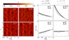 |
Fig. B.1 Comparison of vortex formation in dust-free simulations with varying gas density slope p through corresponding variation of the slope s of the surface mass density. Left: Mid-plane plots of the z-component of the gas vorticity (42) after ~ 1000 orbits. Right: Evolution of the mid-plane gas density. The dashed lines indicate the locations of three large vortices at ~ 1000 orbits. |
References
- ALMA Partnership (Brogan, C. L., et al.) 2015, ApJ, 808, L3 [Google Scholar]
- Andrews, S. M. 2020, ARA&A, 58, 483 [Google Scholar]
- Andrews, S. M., Wilner, D. J., Hughes, A. M., Qi, C., & Dullemond, C. P. 2009, ApJ, 700, 1502 [CrossRef] [Google Scholar]
- Andrews, S. M., Huang, J., Pérez, L. M., et al. 2018, ApJ, 869, L41 [NASA ADS] [CrossRef] [Google Scholar]
- Armitage, P. J. 2011, ARA&A, 49, 195 [Google Scholar]
- Bai, X.-N. 2015, ApJ, 798, 84 [Google Scholar]
- Bai, X.-N. 2017, ApJ, 845, 75 [NASA ADS] [CrossRef] [Google Scholar]
- Bai, X.-N., & Stone, J. M. 2010, ApJ, 722, 1437 [NASA ADS] [CrossRef] [Google Scholar]
- Balbus, S. A., & Hawley, J. F. 1991, ApJ, 376, 214 [Google Scholar]
- Barge, P., & Sommeria, J. 1995, A&A, 295, L1 [NASA ADS] [Google Scholar]
- Barker, A. J., & Latter, H. N. 2015, MNRAS, 450, 21 [NASA ADS] [CrossRef] [Google Scholar]
- Barranco, J. A. 2009, ApJ, 691, 907 [NASA ADS] [CrossRef] [Google Scholar]
- Benítez-Llambay, P., & Masset, F. S. 2016, ApJS, 223, 11 [Google Scholar]
- Benítez-Llambay, P., Krapp, L., & Pessah, M. E. 2019, ApJS, 241, 25 [Google Scholar]
- Blum, J. 2018, Space Sci. Rev., 214, 52 [NASA ADS] [CrossRef] [Google Scholar]
- Carrera, D., Johansen, A., & Davies, M. B. 2015, A&A, 579, A43 [NASA ADS] [CrossRef] [EDP Sciences] [Google Scholar]
- Carrera, D., Simon, J. B., Li, R., Kretke, K. A., & Klahr, H. 2021a, AJ, 161, 96 [Google Scholar]
- Carrera, D., Thomas, A., Simon, J. B., et al. 2021b, ApJ, submitted [arXiv:2108.08315] [Google Scholar]
- Chang, P., & Oishi, J. S. 2010, ApJ, 721, 1593 [NASA ADS] [CrossRef] [Google Scholar]
- Chen, J.-W., & Lin, M.-K. 2018, MNRAS, 478, 2737 [NASA ADS] [CrossRef] [Google Scholar]
- Chiang, E. 2008, ApJ, 675, 1549 [CrossRef] [Google Scholar]
- Crnkovic-Rubsamen, I., Zhu, Z., & Stone, J. M. 2015, MNRAS, 450, 4285 [NASA ADS] [CrossRef] [Google Scholar]
- Flock, M., Nelson, R. P., Turner, N. J., et al. 2017, ApJ, 850, 131 [Google Scholar]
- Flock, M., Turner, N. J., Nelson, R. P., et al. 2020, ApJ, 897, 155 [Google Scholar]
- Fu, W., Li, H., Lubow, S., Li, S., & Liang, E. 2014, ApJ, 795, L39 [NASA ADS] [CrossRef] [Google Scholar]
- Fung, J., & Ono, T. 2021, ApJ, 922, 13 [NASA ADS] [CrossRef] [Google Scholar]
- Gammie, C. F. 1996, ApJ, 457, 355 [Google Scholar]
- Goldreich, P., & Ward, W. R. 1973, ApJ, 183, 1051 [Google Scholar]
- Gressel, O., Turner, N. J., Nelson, R. P., & McNally, C. P. 2015, ApJ, 801, 84 [NASA ADS] [CrossRef] [Google Scholar]
- Haghighipour, N., & Boss, A. P. 2003a, ApJ, 598, 1301 [NASA ADS] [CrossRef] [Google Scholar]
- Haghighipour, N., & Boss, A. P. 2003b, ApJ, 583, 996 [NASA ADS] [CrossRef] [Google Scholar]
- Huang, P., Li, H., Isella, A., et al. 2020, ApJ, 893, 89 [NASA ADS] [CrossRef] [Google Scholar]
- Ishitsu, N., Inutsuka, S.-i., & Sekiya, M. 2009, ArXiv e-prints, [arXiv:0905.4404] [Google Scholar]
- Jacquet, E., Balbus, S., & Latter, H. 2011, MNRAS, 415, 3591 [NASA ADS] [CrossRef] [Google Scholar]
- Johansen, A., & Youdin, A. 2007, ApJ, 662, 627 [Google Scholar]
- Johansen, A., Andersen, A. C., & Brandenburg, A. 2004, A&A, 417, 361 [NASA ADS] [CrossRef] [EDP Sciences] [Google Scholar]
- Johansen, A., Henning, T., & Klahr, H. 2006, ApJ, 643, 1219 [NASA ADS] [CrossRef] [Google Scholar]
- Johansen, A., Youdin, A., & Mac Low, M.-M. 2009a, ApJ, 704, L75 [NASA ADS] [CrossRef] [Google Scholar]
- Johansen, A., Youdin, A., & Klahr, H. 2009b, ApJ, 697, 1269 [Google Scholar]
- Johansen, A., Blum, J., Tanaka, H., et al. 2014, in Protostars and Planets VI, eds. H. Beuther, R. S. Klessen, C. P. Dullemond, & T. Henning, 547 [Google Scholar]
- Kanagawa, K. D., Ueda, T., Muto, T., & Okuzumi, S. 2017, ApJ, 844, 142 [NASA ADS] [CrossRef] [Google Scholar]
- Kenyon, S. J.,& Luu, J. X. 1999, AJ, 118, 1101 [NASA ADS] [CrossRef] [Google Scholar]
- Klahr, H. H., & Bodenheimer, P. 2003, ApJ, 582, 869 [NASA ADS] [CrossRef] [Google Scholar]
- Klahr, H., & Bodenheimer, P. 2006, ApJ, 639, 432 [Google Scholar]
- Klahr, H., & Hubbard, A. 2014, ApJ, 788, 21 [Google Scholar]
- Krapp, L., Benítez-Llambay, P., Gressel, O., & Pessah, M. E. 2019, ApJ, 878, L30 [Google Scholar]
- Krapp, L., Youdin, A. N., Kratter, K. M., & Benítez-Llambay, P. 2020, MNRAS, 497, 2715 [NASA ADS] [CrossRef] [Google Scholar]
- Laibe, G., & Price, D. J. 2014, MNRAS, 440, 2136 [Google Scholar]
- Latter, H. N. 2016, MNRAS, 455, 2608 [NASA ADS] [CrossRef] [Google Scholar]
- Latter, H. N., & Papaloizou, J. 2018, MNRAS, 474, 3110 [NASA ADS] [CrossRef] [Google Scholar]
- Lee, A. T., Chiang, E., Asay-Davis, X., & Barranco, J. 2010, ApJ, 718, 1367 [NASA ADS] [CrossRef] [Google Scholar]
- Lesur, G., & Papaloizou, J. C. B. 2009, A&A, 498, 1 [NASA ADS] [CrossRef] [EDP Sciences] [Google Scholar]
- Lesur, G., & Papaloizou, J. C. B. 2010, A&A, 513, A60 [NASA ADS] [CrossRef] [EDP Sciences] [Google Scholar]
- Lesur, G. R. J., & Latter, H. 2016, MNRAS, 462, 4549 [NASA ADS] [CrossRef] [Google Scholar]
- Li, R., & Youdin, A. 2021, ApJ, 919, 107 [NASA ADS] [CrossRef] [Google Scholar]
- Li, H., Colgate, S. A., Wendroff, B., & Liska, R. 2001, ApJ, 551, 874 [NASA ADS] [CrossRef] [Google Scholar]
- Lin, M.-K. 2019, MNRAS, 485, 5221 [CrossRef] [Google Scholar]
- Lin, M.-K. 2021, ApJ, 907, 64 [Google Scholar]
- Lin, M.-K., & Youdin, A. N. 2015, ApJ, 811, 17 [NASA ADS] [CrossRef] [Google Scholar]
- Lin, M.-K., & Youdin, A. N. 2017, ApJ, 849, 129 [NASA ADS] [CrossRef] [Google Scholar]
- Long, F., Pinilla, P., Herczeg, G. J., et al. 2018, ApJ, 869, 17 [Google Scholar]
- Lorén-Aguilar, P., & Bate, M. R. 2015, MNRAS, 453, L78 [CrossRef] [Google Scholar]
- Lovascio, F., & Paardekooper, S.-J. 2019, MNRAS, 488, 5290 [NASA ADS] [CrossRef] [Google Scholar]
- Lovelace, R. V. E., Li, H., Colgate, S. A., & Nelson, A. F. 1999, ApJ, 513, 805 [NASA ADS] [CrossRef] [Google Scholar]
- Lyra, W. 2014, ApJ, 789, 77 [Google Scholar]
- Lyra, W., & Klahr, H. 2011, A&A, 527, A138 [NASA ADS] [CrossRef] [EDP Sciences] [Google Scholar]
- Lyra, W., Raettig, N., & Klahr, H. 2018, Research Notes of the American Astronomical Society, 2, 195 [NASA ADS] [Google Scholar]
- Manger, N., & Klahr, H. 2018, MNRAS, 480, 2125 [NASA ADS] [CrossRef] [Google Scholar]
- Manger, N., Klahr, H., Kley, W., & Flock, M. 2020, MNRAS, 499, 1841 [NASA ADS] [CrossRef] [Google Scholar]
- Manger, N., Pfeil, T., & Klahr, H. 2021, MNRAS, 508, 5402 [NASA ADS] [CrossRef] [Google Scholar]
- Marcus, P. S., Pei, S., Jiang, C.-H., et al. 2015, ApJ, 808, 87 [NASA ADS] [CrossRef] [Google Scholar]
- Meheut, H., Meliani, Z., Varniere, P., & Benz, W. 2012, A&A, 545, A134 [NASA ADS] [CrossRef] [EDP Sciences] [Google Scholar]
- Miranda, R., Li, H., Li, S., & Jin, S. 2017, ApJ, 835, 118 [NASA ADS] [CrossRef] [Google Scholar]
- Mizuno, H. 1980, Progr. Theor. Phys., 64, 544 [CrossRef] [Google Scholar]
- Nakagawa, Y., Sekiya, M., & Hayashi, C. 1986, Icarus, 67, 375 [Google Scholar]
- Nelson, R. P., Gressel, O., & Umurhan, O. M. 2013, MNRAS, 435, 2610 [Google Scholar]
- Onishi, I. K., & Sekiya, M. 2017, Earth Planets Space, 69, 50 [NASA ADS] [CrossRef] [Google Scholar]
- Ono, T., Muto, T., Takeuchi, T., & Nomura, H. 2016, ApJ, 823, 84 [NASA ADS] [CrossRef] [Google Scholar]
- Paardekooper,S.-J., Lesur, G., & Papaloizou, J. C. B. 2010, ApJ, 725, 146 [Google Scholar]
- Paardekooper, S.-J., McNally, C. P., & Lovascio, F. 2020, MNRAS, 499, 4223 [CrossRef] [Google Scholar]
- Petersen, M. R., Julien, K., & Stewart, G. R. 2007a, ApJ, 658, 1236 [NASA ADS] [CrossRef] [Google Scholar]
- Petersen, M. R., Stewart, G. R., & Julien, K. 2007b, ApJ, 658, 1252 [NASA ADS] [CrossRef] [Google Scholar]
- Pfeil, T., & Klahr, H. 2021, ApJ, 915, 130 [NASA ADS] [CrossRef] [Google Scholar]
- Picogna, G., Stoll, M. H. R., & Kley, W. 2018, A&A, 616, A116 [NASA ADS] [CrossRef] [EDP Sciences] [Google Scholar]
- Raettig, N., Klahr, H., & Lyra, W. 2015, ApJ, 804, 35 [Google Scholar]
- Raettig, N., Lyra, W., & Klahr, H. 2021, ApJ, 913, 92 [NASA ADS] [CrossRef] [Google Scholar]
- Ragusa, E., Dipierro, G., Lodato, G., Laibe, G., & Price, D. J. 2017, MNRAS, 464, 1449 [Google Scholar]
- Railton, A. D., & Papaloizou, J. C. B. 2014, MNRAS, 445, 4409 [Google Scholar]
- Richard, S., Nelson, R. P., & Umurhan, O. M. 2016, MNRAS, 456, 3571 [NASA ADS] [CrossRef] [Google Scholar]
- Safronov, V. S. 1972, Evolution of the protoplanetary cloud and formation of the earth and planets (Keter Publishing House) [Google Scholar]
- Schäfer, U., Johansen, A., & Banerjee, R. 2020, A&A, 635, A190 [Google Scholar]
- Schaffer, N., Johansen, A., & Lambrechts, M. 2021, A&A, 653, A14 [NASA ADS] [CrossRef] [EDP Sciences] [Google Scholar]
- Shakura, N. I., & Sunyaev, R. A. 1973, A&A, 500, 33 [NASA ADS] [Google Scholar]
- Shi, J.-M., & Chiang, E. 2013, ApJ, 764, 20 [NASA ADS] [CrossRef] [Google Scholar]
- Simon, J. B., Armitage, P. J., Li, R., & Youdin, A. N. 2016, ApJ, 822, 55 [Google Scholar]
- Squire, J., & Hopkins, P. F. 2018, MNRAS, 477, 5011 [Google Scholar]
- Stoll, M. H. R., & Kley, W. 2014, A&A, 572, A77 [NASA ADS] [CrossRef] [EDP Sciences] [Google Scholar]
- Stoll, M. H. R., & Kley, W. 2016, A&A, 594, A57 [NASA ADS] [CrossRef] [EDP Sciences] [Google Scholar]
- Stoll, M. H. R., Kley, W., & Picogna, G. 2017, A&A, 599, L6 [NASA ADS] [CrossRef] [EDP Sciences] [Google Scholar]
- Surville, C., & Mayer, L. 2019, ApJ, 883, 176 [NASA ADS] [CrossRef] [Google Scholar]
- Takeuchi, T., & Lin, D. N. C. 2002, ApJ, 581, 1344 [NASA ADS] [CrossRef] [Google Scholar]
- Taki, T., Fujimoto, M., & Ida, S. 2016, A&A, 591, A86 [NASA ADS] [CrossRef] [EDP Sciences] [Google Scholar]
- Tassoul, J. 1978, Theory of rotating stars (Princeton: University Press) [Google Scholar]
- Turner, N. J., & Drake, J. F. 2009, ApJ, 703, 2152 [NASA ADS] [CrossRef] [Google Scholar]
- Turner, N. J., Fromang, S., Gammie, C., et al. 2014, in Protostars and Planets VI, eds. H. Beuther, R. S. Klessen, C. P. Dullemond, & T. Henning, 411 [Google Scholar]
- Urpin, V. 2003, A&A, 404, 397 [NASA ADS] [CrossRef] [EDP Sciences] [Google Scholar]
- Urpin, V., & Brandenburg, A. 1998, MNRAS, 294, 399 [Google Scholar]
- van der Marel,N., van Dishoeck, E. F., Bruderer, S., et al. 2013, Science, 340, 1199 [NASA ADS] [CrossRef] [Google Scholar]
- van der Marel,N., Birnstiel, T., Garufi, A., et al. 2021, AJ, 161, 33 [Google Scholar]
- Weidenschilling, S. J. 1977, MNRAS, 180, 57 [Google Scholar]
- Weidenschilling, S. J., & Cuzzi, J. N. 1993, in Protostars and Planets III, eds. E. H. Levy & J. I. Lunine, 1031 [Google Scholar]
- Wetherill, G. W. 1990, Bull. Am. Astron. Soc., 22, 1335 [Google Scholar]
- Yang, C. C., Johansen, A., & Carrera, D. 2017, A&A, 606, A80 [NASA ADS] [CrossRef] [EDP Sciences] [Google Scholar]
- Youdin, A. N., & Goodman, J. 2005, ApJ, 620, 459 [Google Scholar]
- Youdin, A., & Johansen, A. 2007, ApJ, 662, 613 [Google Scholar]
- Zhu, Z., & Stone, J. M. 2014, ApJ, 795, 53 [Google Scholar]
- Zhu, Z., & Yang, C.-C. 2021, MNRAS, 501, 467 [Google Scholar]
Strictly cs should be replaced by the mean thermal gas velocity (Weidenschilling 1977) which differs from cs by a factor
 . For convenience we absorb this factor in the particle size rd.
In what follows we restrict to values z > 0, keeping in mind that a similar argument applies to the case z < 0.
In these test simulations we adopted a very small temperature gradient q → 0 such that the VSI was extinguished.
A similar result is obtained with A = 0.2.
All Tables
All Figures
|
Fig. 1 Illustration of the initial mid-plane gas density profile (top panel) according to Eq. (32) and the dust drift velocities (bottom panel) computed from (36) with τ0 = 10−2 for different pressure bump amplitudes A. |
| In the text | |
|
Fig. 2 Time evolution of quantities that describe the dust settling process against the emergence of VSI turbulence. From top to bottom these are the ratio of dust-to-gas scale height, the mid-plane dust-to-gas density ratio, the root mean squared mid-plane vertical gas velocity, and the root mean squared (rms) vertical Reynolds stress. The left panels compare different metallicities with fixed τ0 = 10−3, while the right panels compare different Stokes numbers τ0 with Z = 0.01. The dashed red lines in the panels of rms(vgz0) are the exponential |
| In the text | |
|
Fig. 3 2D simulation survey of the effect of a pressure bump on dust evolution. Shown is the final location of
|
| In the text | |
|
Fig. 4 Time evolution of the dust-to-gas ratio in the vicinity of a pressure bump with amplitude A = 0.4. Compared from left to right are different metallicities Z = 0.01, 0.03, 0.05 with the same τ0 = 4 × 10⁻³. The over-plotted solid curves are the mid-plane gas pressure at times indicated by horizontal dashed lines. The dashed curves are the initial gas pressure for comparison. The arrows indicate the direction of dust movement as predicted by Eq. (36) and are all normalized to have the same length. |
| In the text | |
|
Fig. 5 Meridional cuts of (from top to bottom) the dust-to-gas ratio at 450 orbits, the averaged Solberg–Høiland expressions (39), (40) (the left hand side terms) and root mean squared vertical Reynolds stress. Averages are taken over the time 350–450 orbits. In the panels ⟨SH1 ⟩ and ⟨SH2⟩, negative values are indicated by a black color. These plots compare the same simulations as in Fig. 4 and illustrate the emergence of a dusty gas instability through a violation of the Solberg–Høiland criteria. |
| In the text | |
|
Fig. 6 Comparison of the vertical Reynolds stress (43) in 2D and 3D simulations for different metallicities, Z, and Stokes numbers, τ0. Upper panels: running time-averages (spatially averaged over the entire diagnostic domain 0.8 ≤ R ≤ 1.2), while the lower panels display the time-averaged (over the last 400 orbits) vertical profiles. The dashed curve is in all panels for 2D and 3D the same, respectively. The horizontal dotted line indicates “zero”, such that positive and negative values correspond to angular momentum transport away from the mid-plane and towards the mid-pane, respectively. |
| In the text | |
|
Fig. 7 Illustration of the origin of the increased vertical Reynolds stress |
| In the text | |
|
Fig. 8 Vertical profiles of the averaged radial dust and gas velocities (upper three rows) and the dust and gas mass flows (lower three rows) in 3D (left panels) and 2D (right panels) simulations. The Stokes number τ0 increases from left to right while Z increases from the lower to upper panels. For comparison, in the panels corresponding to Z = 0.01 and τ0 = 10−3 we additionally plot the result of a dust-free simulation. Averages have been taken over the last 400 orbits and over 0.8 ≤ R ≤ 1.2. The dust mass flows are additionally scaled with a factor 1∕ϵ0 as compared to the gas mass flows. The horizontal axis displays − 2Hg ≤ z ≤ 2Hg in all panels. |
| In the text | |
|
Fig. 9 Meridional plots of the time-averaged Reynolds stress |
| In the text | |
|
Fig. 10 Comparison of the dust settling process in 2D and 3D simulations for different metallicities Z and Stokes numbers τ0. Shown are the ratios of the dust and gas scale heights (upper panels) and the mid-plane dust and gas densities. All quantities are averaged in radius and in 3D simulations also in φ. |
| In the text | |
|
Fig. 11 α-viscosity parameter (45) as measured in 3D simulations for different metallicities and Stokes numbers. The dotted curves correspond to a dust-free simulation. The upper panels display the running time-average of the spatially averaged value while the lower panels show vertical profiles, averaged in time. |
| In the text | |
|
Fig. 12 Snap shots of dust-to-gas density ratio at late times (800−1000 orbits) in simulations including a pressure bump with amplitude A = 0.2 and with Stokes number τ0 = 10−3. The dashed and dotted curves represent the initial and final mid-plane gas pressure profiles, respectively. |
| In the text | |
|
Fig. 13 Snap shots of dust-to-gas density ratio at late times (800−1000 orbits) in simulations including a pressure bump with amplitude A = 0.2 and with Stokes number τ0 = 10−2. The dashed and dotted curves represent the initial and final mid-plane gas pressure profiles, respectively. |
| In the text | |
|
Fig. 14 Snap shots of dust-to-gas density ratio at late times (800−1000 orbits) in simulations including a pressure bump with amplitude A = 0.4 and with Stokes number τ0 = 10−3. The dashed and dotted curves represent the initial and final mid-plane gas pressure profiles, respectively. |
| In the text | |
|
Fig. 15 Snap shots of dust-to-gas density ratio at late times (800–1000 orbits) in simulations including a pressure bump with amplitude A = 0.4 and with Stokes number τ0 = 10−2. The dashed and dotted curves represent the initial and final mid-plane gas pressure profiles, respectively. |
| In the text | |
|
Fig. 16 Radial locations of dust rings in 3D (solid curves) and 2D (dashed curves) simulations for metallicities Z = 0.01 (black curves), and Z = 0.03 (red curves) and bump amplitudes A = 0.2 (thin curves)and A = 0.4 (thick curves). The locations correspond to the maximum value of ϵ at each time. The sporadic reversals of the drift direction are due to turbulent fluctuations of the dust density within the rings. The 3D simulations are the same as in Figs. 13 and 15. The 2D simulations are those shownin Fig. 3. |
| In the text | |
|
Fig. 17 Time evolution of an unstable dust ring in a 3D simulation with parameters τ0 = 4 × 10⁻³, Z = 0.03, and A = 0.4. The dashed and solid curves are the initial and current mid-plane gas pressure profile, respectively. One can clearly see an amplification of the gas pressure bump and unstable behavior of the dust ring, as it develops strong non-axisymmetries and splits ofa vortex which subsequently migrates inward. |
| In the text | |
|
Fig. 18 Mid-plane plots of the z-component of the gas vorticity Eq. (42) after 540 orbits in dust-free simulations with an initial pressure bump of varying amplitude A. |
| In the text | |
|
Fig. 19 Evolution of the mid-plane gas density for dust-free simulations with an initial pressure bump of varying amplitude A. The dashed lines indicate the location of the large vortex in these simulations at the three latest times. |
| In the text | |
|
Fig. 20 Radial profiles (azimuthally averaged) of the vortensity (41) at different times in simulations with Stokes number τ0 = 10−3 and different metallicities Z. The occurrence of sharp peaks in this quantity suggests that the smallest scale structures appearing in our simulations are most likely not sufficiently resolved in order to properly compute numerical derivatives contained in the quantity
|
| In the text | |
|
Fig. 21 Evolution of the mid-plane gas density in dusty simulations with different metallicity Z, Stokes number τ0 and pressurebump amplitude A. |
| In the text | |
|
Fig. 22 Example evolution of large dusty vortices that formed at a pressure bump (A = 0.4) in 3D simulations with metallicity Z = 0.01 and Stokes numbers τ0 = 10−3 (upper panels) and τ0 = 10−2 (lower panels). The contour plots show the dust-to-gas ratio. The insert plot displays the vortex location (black curve) and its maximum dust-to-gas ratio (red curve) as functions of time. |
| In the text | |
|
Fig. 23 Detailed view of the large dusty vortex corresponding to the upper panels of Fig. 22. Snapshots of the dust-to-gas ratio (lower left panel), the dust-to-gas scale height ratio (middle left panel) and the mid-plane gas pressure scaled with its azimuthally averaged value at each radius are shown. The right panels show the dust vorticity (42) at different heights (z = 0 in the lowerright panel). The arrows in the lower right panel illustrate the dust velocity in the frame co-moving with the Keplerian shear and where in addition the spatial average of the azimuthal velocity over the displayed region has been subtracted to suppress the contribution of the vortex bulk motion. |
| In the text | |
|
Fig. A.1 Time evolution of the dust-to-gas ratio in the vicinity of a pressure bump with amplitude A = 0.4. Compared from left to right are different temperature slopes q, with the same metallicity Z = 0.01 and Stokes number τ0 = 6 ⋅ 10−3. The over-plotted solid curves are the mid-plane gas pressure at times indicated by horizontal dashed lines. The dashed curves are the initial gas pressure for comparison. The arrows indicate the direction of dust movement as predicted by Equation (36) and are all normalized to have the same length. |
| In the text | |
|
Fig. A.2 Time evolution of the dust-to-gas ratio in the vicinity of a pressure bump with amplitude A = 0.4. Compared from left to right are different temperature slopes q, with the same metallicity Z = 0.03 and Stokes number τ0 = 6 ⋅ 10−3. The over-plotted solid curves are the mid-plane gas pressure at times indicated by horizontal dashed lines. The dashed curves are the initial gas pressure for comparison. The arrows indicate the direction of dust movement as predicted by Equation (36) and are all normalized to have the same length. |
| In the text | |
|
Fig. B.1 Comparison of vortex formation in dust-free simulations with varying gas density slope p through corresponding variation of the slope s of the surface mass density. Left: Mid-plane plots of the z-component of the gas vorticity (42) after ~ 1000 orbits. Right: Evolution of the mid-plane gas density. The dashed lines indicate the locations of three large vortices at ~ 1000 orbits. |
| In the text | |
Current usage metrics show cumulative count of Article Views (full-text article views including HTML views, PDF and ePub downloads, according to the available data) and Abstracts Views on Vision4Press platform.
Data correspond to usage on the plateform after 2015. The current usage metrics is available 48-96 hours after online publication and is updated daily on week days.
Initial download of the metrics may take a while.