| Issue |
A&A
Volume 658, February 2022
|
|
|---|---|---|
| Article Number | A20 | |
| Number of page(s) | 14 | |
| Section | Cosmology (including clusters of galaxies) | |
| DOI | https://doi.org/10.1051/0004-6361/202142073 | |
| Published online | 26 January 2022 | |
Euclid: Forecasts from redshift-space distortions and the Alcock–Paczynski test with cosmic voids⋆
1
Universitäts-Sternwarte München, Fakultät für Physik, Ludwig-Maximilians-Universität München, Scheinerstrasse 1, 81679 München, Germany
e-mail: This email address is being protected from spambots. You need JavaScript enabled to view it.
2
University of Lyon, UCB Lyon 1, CNRS/IN2P3, IUF, IP2I, Lyon, France
3
Aix-Marseille Univ., CNRS/IN2P3, CPPM, Marseille, France
4
Department of Astrophysical Sciences, Peyton Hall, Princeton University, Princeton, NJ 08544, USA
5
Dipartimento di Fisica e Astronomia “Augusto Righi” – Alma Mater Studiorum Universitá di Bologna, Viale Berti Pichat 6/2, 40127 Bologna, Italy
6
INFN-Sezione di Bologna, Viale Berti Pichat 6/2, 40127 Bologna, Italy
7
INAF-IASF Bologna, Via Piero Gobetti 101, 40129 Bologna, Italy
8
INFN-Padova, Via Marzolo 8, 35131 Padova, Italy
9
Dipartimento di Fisica e Astronomia “G. Galilei”, Universitá di Padova, Via Marzolo 8, 35131 Padova, Italy
10
Sorbonne Universités, UPMC Univ. Paris 6 et CNRS, UMR 7095, Institut d’Astrophysique de Paris, 98bis bd Arago, 75014 Paris, France
11
Max Planck Institute for Extraterrestrial Physics, Giessenbachstr. 1, 85748 Garching, Germany
12
INFN-Sezione di Genova, Via Dodecaneso 33, 16146 Genova, Italy
13
Dipartimento di Fisica, Universitá degli Studi di Genova, and INFN-Sezione di Genova, Via Dodecaneso 33, 16146 Genova, Italy
14
INFN-Sezione di Milano, Via Celoria 16, 20133 Milano, Italy
15
INAF-IASF Milano, Via Alfonso Corti 12, 20133 Milano, Italy
16
Dipartimento di Fisica “Aldo Pontremoli”, Universitá degli Studi di Milano, Via Celoria 16, 20133 Milano, Italy
17
INAF-Osservatorio Astronomico di Brera, Via Brera 28, 20122 Milano, Italy
18
Universidad de la Laguna, 38206 San Cristóbal de La Laguna, Tenerife, Spain
19
Instituto de Astrofísica de Canarias, Calle Vía Làctea s/n, 38204 San Cristòbal de la Laguna, Tenerife, Spain
20
Dipartimento di Fisica e Astronomia “Augusto Righi” – Alma Mater Studiorum Universitá di Bologna, Via Piero Gobetti 93/2, 40129 Bologna, Italy
21
INAF-Osservatorio di Astrofisica e Scienza dello Spazio di Bologna, Via Piero Gobetti 93/3, 40129 Bologna, Italy
22
Department of Physics and Astronomy, University of Waterloo, Waterloo, Ontario N2L 3G1, Canada
23
Centre for Astrophysics, University of Waterloo, Waterloo, Ontario N2L 3G1, Canada
24
Perimeter Institute for Theoretical Physics, Waterloo, Ontario N2L 2Y5, Canada
25
Institute of Theoretical Astrophysics, University of Oslo, PO Box 1029 Blindern, 0315 Oslo, Norway
26
Swedish Collegium for Advanced Study, Thunbergsvägen 2, 752 38 Uppsala, Sweden
27
Theoretical Astrophysics, Department of Physics and Astronomy, Uppsala University, Box 515, 751 20 Uppsala, Sweden
28
Université St Joseph, UR EGFEM, Faculty of Sciences, Beirut, Lebanon
29
Institut de Recherche en Astrophysique et Planétologie (IRAP), Université de Toulouse, CNRS, UPS, CNES, 14 Av. Edouard Belin, 31400 Toulouse, France
30
Mullard Space Science Laboratory, University College London, Holmbury St Mary, Dorking, Surrey RH5 6NT, UK
31
INAF-Osservatorio Astrofisico di Torino, Via Osservatorio 20, 10025 Pino Torinese, TO, Italy
32
INFN-Sezione di Roma Tre, Via della Vasca Navale 84, 00146 Roma, Italy
33
Department of Mathematics and Physics, Roma Tre University, Via della Vasca Navale 84, 00146 Rome, Italy
34
INAF-Osservatorio Astronomico di Capodimonte, Via Moiariello 16, 80131 Napoli, Italy
35
Instituto de Astrofísica e Ciências do Espaço, Universidade do Porto, CAUP, Rua das Estrelas, 4150-762 Porto, Portugal
36
Port d’Informació Científica, Campus UAB, C. Albareda s/n, 08193 Bellaterra, Barcelona, Spain
37
Institut de Física d’Altes Energies (IFAE), The Barcelona Institute of Science and Technology, Campus UAB, 08193 Bellaterra, Barcelona, Spain
38
Institute of Space Sciences (ICE, CSIC), Campus UAB, Carrer de Can Magrans, s/n, 08193 Barcelona, Spain
39
Institut d’Estudis Espacials de Catalunya (IEEC), Carrer Gran Capitá 2-4, 08034 Barcelona, Spain
40
INAF-Osservatorio Astronomico di Roma, Via Frascati 33, 00078 Monteporzio Catone, Italy
41
Department of Physics “E. Pancini”, University Federico II, Via Cinthia 6, 80126 Napoli, Italy
42
INFN Section of Naples, Via Cinthia 6, 80126 Napoli, Italy
43
INAF-Osservatorio Astrofisico di Arcetri, Largo E. Fermi 5, 50125 Firenze, Italy
44
Institut National de Physique Nucléaire et de Physique des Particules, 3 rue Michel-Ange, 75794 Paris Cedex 16, France
45
Centre National d’Etudes Spatiales, Toulouse, France
46
Institute for Astronomy, University of Edinburgh, Royal Observatory, Blackford Hill, Edinburgh EH9 3HJ, UK
47
European Space Agency/ESRIN, Largo Galileo Galilei 1, 00044 Frascati, Roma, Italy
48
ESAC/ESA, Camino Bajo del Castillo, s/n., Urb. Villafranca del Castillo, 28692 Villanueva de la Cañada, Madrid, Spain
49
Univ. Lyon, Univ. Claude Bernard Lyon 1, CNRS/IN2P3, IP2I Lyon, UMR 5822, 69622 Villeurbanne, France
50
Departamento de Física, Faculdade de Ciências, Universidade de Lisboa, Edifício C8, Campo Grande, 1749-016 Lisboa, Portugal
51
Instituto de Astrofísica e Ciências do Espaço, Faculdade de Ciências, Universidade de Lisboa, Campo Grande, 1749-016 Lisboa, Portugal
52
Department of Astronomy, University of Geneva, ch. d’Ecogia 16, 1290 Versoix, Switzerland
53
Université Paris-Saclay, CNRS, Institut d’Astrophysique Spatiale, 91405 Orsay, France
54
Department of Physics, Oxford University, Keble Road, Oxford OX1 3RH, UK
55
INAF-Osservatorio Astronomico di Trieste, Via G. B. Tiepolo 11, 34131 Trieste, Italy
56
Istituto Nazionale di Astrofisica (INAF) – Osservatorio di Astrofisica e Scienza dello Spazio (OAS), Via Gobetti 93/3, 40127 Bologna, Italy
57
Istituto Nazionale di Fisica Nucleare, Sezione di Bologna, Via Irnerio 46, 40126 Bologna, Italy
58
INAF-Osservatorio Astronomico di Padova, Via dell’Osservatorio 5, 35122 Padova, Italy
59
Jet Propulsion Laboratory, California Institute of Technology, 4800 Oak Grove Drive, Pasadena, CA 91109, USA
60
von Hoerner & Sulger GmbH, SchloßPlatz 8, 68723 Schwetzingen, Germany
61
Max-Planck-Institut für Astronomie, Königstuhl 17, 69117 Heidelberg, Germany
62
AIM, CEA, CNRS, Université Paris-Saclay, Université de Paris, 91191 Gif-sur-Yvette, France
63
Université de Genève, Département de Physique Théorique and Centre for Astroparticle Physics, 24 quai Ernest-Ansermet, 1211 Genève 4, Switzerland
64
Department of Physics and Helsinki Institute of Physics, University of Helsinki, Gustaf Hällströmin katu 2, 00014 Helsinki, Finland
65
NOVA Optical Infrared Instrumentation Group at ASTRON, Oude Hoogeveensedijk 4, 7991 PD Dwingeloo, The Netherlands
66
Argelander-Institut für Astronomie, Universität Bonn, Auf dem Hügel 71, 53121 Bonn, Germany
67
Institute for Computational Cosmology, Department of Physics, Durham University, South Road, Durham DH1 3LE, UK
68
Université Côte d’Azur, Observatoire de la Côte d’Azur, CNRS, Laboratoire Lagrange, Bd de l’Observatoire, CS 34229, 06304 Nice Cedex 4, France
69
University of Applied Sciences and Arts of Northwestern Switzerland, School of Engineering, 5210 Windisch, Switzerland
70
California Institute of Technology, 1200 E California Blvd, Pasadena, CA 91125, USA
71
Institute of Physics, Laboratory of Astrophysics, Ecole Polytechnique Fédérale de Lausanne (EPFL), Observatoire de Sauverny, 1290 Versoix, Switzerland
72
European Space Agency/ESTEC, Keplerlaan 1, 2201 AZ Noordwijk, The Netherlands
73
Department of Physics and Astronomy, University of Aarhus, Ny Munkegade 120, 8000 Aarhus C, Denmark
74
Institute of Space Science, Bucharest 077125, Romania
75
Departamento de Astrofísica, Universidad de La Laguna, 38206 La Laguna, Tenerife, Spain
76
Centro de Investigaciones Energéticas, Medioambientales y Tecnológicas (CIEMAT), Avenida Complutense 40, 28040 Madrid, Spain
77
Instituto de Astrofísica e Ciências do Espaço, Faculdade de Ciências, Universidade de Lisboa, Tapada da Ajuda, 1349-018 Lisboa, Portugal
78
Universidad Politécnica de Cartagena, Departamento de Electrónica y Tecnología de Computadoras, 30202 Cartagena, Spain
79
Kapteyn Astronomical Institute, University of Groningen, PO Box 800 9700 AV Groningen, The Netherlands
80
Infrared Processing and Analysis Center, California Institute of Technology, Pasadena, CA 91125, USA
81
Dipartimento di Fisica e Astronomia, Universitá di Bologna, Via Gobetti 93/2, 40129 Bologna, Italy
82
INFN-Sezione di Torino, Via P. Giuria 1, 10125 Torino, Italy
83
Dipartimento di Fisica, Universitá degli Studi di Torino, Via P. Giuria 1, 10125 Torino, Italy
84
Université de Paris, CNRS, Astroparticule et Cosmologie, 75013 Paris, France
Received:
23
August
2021
Accepted:
31
October
2021
Abstract
Euclid is poised to survey galaxies across a cosmological volume of unprecedented size, providing observations of more than a billion objects distributed over a third of the full sky. Approximately 20 million of these galaxies will have their spectroscopy available, allowing us to map the three-dimensional large-scale structure of the Universe in great detail. This paper investigates prospects for the detection of cosmic voids therein and the unique benefit they provide for cosmological studies. In particular, we study the imprints of dynamic (redshift-space) and geometric (Alcock–Paczynski) distortions of average void shapes and their constraining power on the growth of structure and cosmological distance ratios. To this end, we made use of the Flagship mock catalog, a state-of-the-art simulation of the data expected to be observed with Euclid. We arranged the data into four adjacent redshift bins, each of which contains about 11 000 voids and we estimated the stacked void-galaxy cross-correlation function in every bin. Fitting a linear-theory model to the data, we obtained constraints on f/b and DMH, where f is the linear growth rate of density fluctuations, b the galaxy bias, DM the comoving angular diameter distance, and H the Hubble rate. In addition, we marginalized over two nuisance parameters included in our model to account for unknown systematic effects in the analysis. With this approach, Euclid will be able to reach a relative precision of about 4% on measurements of f/b and 0.5% on DMH in each redshift bin. Better modeling or calibration of the nuisance parameters may further increase this precision to 1% and 0.4%, respectively. Our results show that the exploitation of cosmic voids in Euclid will provide competitive constraints on cosmology even as a stand-alone probe. For example, the equation-of-state parameter, w, for dark energy will be measured with a precision of about 10%, consistent with previous more approximate forecasts.
Key words: cosmology: observations / cosmological parameters / dark energy / large-scale structure of Universe / methods: data analysis / surveys
This paper is published on behalf of the Euclid Consortium.
© ESO 2022
1. Introduction
The formation of cosmic voids in the large-scale structure of the Universe is a consequence of the gravitational interaction of its initially smooth distribution of matter eventually evolving into collapsed structures that make up the cosmic web (Zeldovich 1970). This process leaves behind vast regions of nearly empty space that constitute the largest known structures in the Universe. Since their first discovery in the late 1970s (Gregory & Thompson 1978; Jõeveer et al. 1978), cosmic voids have intrigued scientists given their peculiar nature (e.g., Kirshner et al. 1981; Bertschinger 1985; White et al. 1987; van de Weygaert & van Kampen 1993; Peebles 2001). However, only the recent advances in surveys, such as 6dFGS (Jones et al. 2004), BOSS (Dawson et al. 2013), DES (The Dark Energy Survey Collaboration 2005), eBOSS (Dawson et al. 2016), KiDS (de Jong et al. 2013), SDSS (Eisenstein et al. 2011), and VIPERS (Guzzo et al. 2014), have enabled systematic studies of statistically significant sample sizes (e.g., Pan et al. 2012; Sutter et al. 2012a), placing the long-overlooked field of cosmic voids into a new focus of interest in astronomy. In conjunction with the extensive development of large simulations (e.g., Springel 2005; Schaye et al. 2015; Dolag et al. 2016; Potter et al. 2017), this has sparked a plethora of studies on voids and their connection to galaxy formation (Hoyle et al. 2005; Patiri et al. 2006; Kreckel et al. 2012; Ricciardelli et al. 2014; Habouzit et al. 2020; Panchal et al. 2020), large-scale structure (Sheth & van de Weygaert 2004; Hahn et al. 2007; van de Weygaert & Schaap 2009; Jennings et al. 2013; Hamaus et al. 2014a; Chan et al. 2014; Voivodic et al. 2020), the nature of gravity (Clampitt et al. 2013; Zivick et al. 2015; Cai et al. 2015; Barreira et al. 2015; Achitouv 2016; Voivodic et al. 2017; Falck et al. 2018; Sahlén & Silk 2018; Baker et al. 2018; Paillas et al. 2019; Davies et al. 2019; Perico et al. 2019; Alam et al. 2021; Contarini et al. 2021; Wilson & Bean 2021), properties of dark matter (Leclercq et al. 2015; Yang et al. 2015; Reed et al. 2015; Baldi & Villaescusa-Navarro 2018), dark energy (Lee & Park 2009; Bos et al. 2012; Spolyar et al. 2013; Pisani et al. 2015a; Pollina et al. 2016; Verza et al. 2019), massive neutrinos (Massara et al. 2015; Banerjee & Dalal 2016; Sahlén 2019; Kreisch et al. 2019; Schuster et al. 2019; Zhang et al. 2020; Bayer et al. 2021), inflation (Chan et al. 2019), and cosmology in general (Lavaux & Wandelt 2012; Sutter et al. 2012b; Hamaus et al. 2014b, 2016, 2020; Correa et al. 2019, 2022; Contarini et al. 2019; Nadathur et al. 2019, 2020; Paillas et al. 2021; Kreisch et al. 2021). We refer to Pisani et al. (2019) for a more extensive recent summary.
From an observational perspective, voids are an abundant structure type that, together with halos, filaments, and walls, build up the cosmic web. It is therefore natural to utilize them in the search for those observables that have traditionally been measured via galaxies or galaxy clusters, which trace the overdense regions of large-scale structure. This strategy has proven itself to be very promising in recent years, uncovering a treasure trove of untapped signals that carry cosmologically relevant information, such as the integrated Sachs–Wolfe (ISW; Granett et al. 2008; Cai et al. 2010, 2014; Ilić et al. 2013; Nadathur & Crittenden 2016; Kovács & García-Bellido 2016; Kovács et al. 2019), Sunyaev–Zeldovich (SZ; Alonso et al. 2018), and Alcock–Paczynski (AP) effects (Sutter et al. 2012b, 2014a; Hamaus et al. 2016; Mao et al. 2017; Nadathur et al. 2019), as well as gravitational lensing (Melchior et al. 2014; Clampitt & Jain 2015; Gruen et al. 2016; Sánchez et al. 2017a; Cai et al. 2017; Chantavat et al. 2017; Brouwer et al. 2018; Fang et al. 2019), baryon acoustic oscillations (BAO; Kitaura et al. 2016; Liang et al. 2016; Chan & Hamaus 2021; Forero-Sánchez et al. 2021), and redshift-space distortions (RSD; Paz et al. 2013; Cai et al. 2016; Hamaus et al. 2017; Hawken et al. 2017, 2020; Achitouv 2019; Aubert et al. 2020). The aim of this paper is to forecast the constraining power on cosmological parameters with a combined analysis of RSD and the AP effect from voids available in Euclid. As proposed in Hamaus et al. (2015) and carried out with BOSS data in Hamaus et al. (2016) for the first time, this combined approach allows simultaneous constraints on the expansion history of the Universe and the growth rate of structure inside it.
The Euclid satellite mission is a “Stage-IV” dark energy experiment (Albrecht et al. 2006) that will outperform current surveys in the number of observed galaxies and in coverage of cosmological volume (Laureijs et al. 2011). Scheduled for launch in 2022, an assessment of its science performance is timely (Amendola et al. 2018; Euclid Collaboration 2020) and the scientific return that can be expected from voids is being investigated in a series of companion papers within the Euclid Collaboration. These papers cover different observables, such as the void size function (Contarini et al., in prep.), the void-galaxy cross-correlation function after velocity-field reconstruction (Radinović et al., in prep.), or void lensing (Bonici et al., in prep.), providing independent forecasts on their cosmological constraining power. In this paper, we present a mock-data analysis of the stacked void-galaxy cross-correlation function in redshift space based on the Flagship simulation (Potter et al. 2017), which provides realistic galaxy catalogs as expected to be observed with Euclid. In the following, we outline the theoretical background in Sect. 2, describe the mock data in Sect. 3, and present our results in Sect. 4. The implications of our findings are then discussed in Sect. 5 and our conclusions are summarized in Sect. 6.
2. Theoretical background
According to the cosmological principle, the Universe obeys homogeneity and isotropy on very large scales, which is supported by recent observations (e.g., Scrimgeour et al. 2012; Laurent et al. 2016; Ntelis et al. 2017; Gonçalves et al. 2021). However, below the order of 102 Mpc scales, we observe the structures that form the cosmic web, which break these symmetries locally. Nevertheless, the principle is still valid on those scales in a statistical sense, that is, for an ensemble average over patches of similar extent from different locations in the Universe. If the physical size of such patches is known (a so-called standard ruler), this enables an inertial observer to determine cosmological distances and the expansion history. The BAO feature in the galaxy distribution is a famous example for a standard ruler, it has been exploited for distance measurements with great success in the past (e.g., Alam et al. 2017, 2021) and constitutes one of the main cosmological probes of Euclid (Laureijs et al. 2011).
A related approach may be pursued with so-called standard spheres, namely, patches of a known physical shape (in particular, spherically symmetric ones). This method has originally been proposed by Alcock & Paczynski (1979, hereafter AP) as a probe of the expansion history, it was later demonstrated that voids are well suited for this type of experiment (Ryden 1995; Lavaux & Wandelt 2012). In principle, it applies to any type of structure in the Universe that exhibits random orientations (such as halos, filaments, or walls), which necessarily results in a spherically symmetric ensemble average. However, the expansion history can only be probed with structures that have not decoupled from the Hubble flow via gravitational collapse. Furthermore, spherical symmetry is broken by peculiar line-of-sight motions of the observed objects that make up this structure. These cause a Doppler shift in the received spectrum and, hence, affect the redshift-distance relation to the source (Kaiser 1987). In order to apply the AP test, one has to account for those RSD, which requires the modeling of peculiar velocities. For the complex phase-space structure of halos, respectively galaxy clusters as their observational counterparts, this is a very challenging problem. For filaments and walls, the situation is only marginally improved, since they have experienced shell crossing in at least one dimension. On the other hand, voids have hardly undergone any shell crossing in their interiors (Shandarin 2011; Abel et al. 2012; Sutter et al. 2014b; Hahn et al. 2015), providing an environment that is characterized by a coherent flow of matter and on that is therefore very amenable to dynamical models.
In fact, with the help of N-body simulations, it has been shown that local mass conservation provides a very accurate description, even at linear order in the density fluctuations (Hamaus et al. 2014c). In that case, the velocity field u relative to the void center is given by (Peebles 1980)
 (1)
(1)
where r is the comoving real-space distance vector to the void center, H(z) the Hubble rate at redshift z, f(z) is the linear growth rate of density perturbations δ, and Δ(r) is the average matter-density contrast enclosed in a spherical region of radius r:
 (2)
(2)
The comoving distance vector s in redshift space receives an additional contribution from the line-of-sight component of u (indicated by u∥), caused by the Doppler effect,
 (3)
(3)
This equation determines the mapping between real and redshift space at linear order. Its Jacobian can be expressed analytically and yields a relation between the void-galaxy cross-correlation functions ξ in both spaces (a superscript s indicates redshift space),
![Mathematical equation: $$ \begin{aligned} \xi ^s(\boldsymbol{s}) \simeq \xi (r) + \frac{f}{3}\Delta (r) + f\mu ^2[\delta (r)-\Delta (r)], \end{aligned} $$](/articles/aa/full_html/2022/02/aa42073-21/aa42073-21-eq4.gif) (4)
(4)
where μ = r∥/r denotes the cosine of the angle between r and the line of sight (see Cai et al. 2016; Hamaus et al. 2017, 2020, for a more detailed derivation). The real-space quantities ξ(r), δ(r) and its integral Δ(r) on the right-hand side of Eq. (4) are a priori unknown, but they can be related to the observables with some basic assumptions. Firstly, ξ(r) can be obtained via deprojection of the projected void-galaxy cross-correlation function  in redshift space (Pisani et al. 2014; Hawken et al. 2017),
 (5)
(5)
By construction  is insensitive to RSD, since the line-of-sight component s∥ is integrated out in its definition and the projected separation s⊥ on the plane of the sky is identical to its real-space counterpart r⊥,
 (6)
(6)
Equations (5) and (6) are also referred to as inverse and forward Abel transform, respectively (Abel et al. 1842; Bracewell 1999).
Secondly, the matter fluctuation δ(r) around the void center can be related to ξ(r) assuming a bias relation for the galaxies in that region. Based on simulation studies, it has been demonstrated that a linear relation of the form ξ(r) = bδ(r) with a proportionality constant b serves that purpose with sufficiently high accuracy. Moreover, it has been shown that the value of b is linearly related to the large-scale linear galaxy bias of the tracer distribution, and coincides with it for sufficiently large voids (Sutter et al. 2014c; Pollina et al. 2017, 2019; Contarini et al. 2019; Ronconi et al. 2019). With this, Eq. (4) can be expressed as
![Mathematical equation: $$ \begin{aligned} \xi ^s(\boldsymbol{s}) \simeq \xi (r) + \frac{1}{3}\frac{f}{b}\overline{\xi }(r) + \frac{f}{b}\mu ^2[{\xi (r)-\overline{\xi }(r)}], \end{aligned} $$](/articles/aa/full_html/2022/02/aa42073-21/aa42073-21-eq9.gif) (7)
(7)
where
 (8)
(8)
Now, together with Eq. (3) to relate real and redshift-space coordinates, Eq. (7) provides a description of the observable void-galaxy cross-correlation function at linear order in perturbation theory.
In order to determine the distance vector s for a given void-galaxy pair, it is necessary to convert their observed separation in angle δϑ and redshift δz to comoving distances via
 (9)
(9)
where DM(z) is the comoving angular diameter distance. Both H(z) and DM(z) depend on cosmology, so any evaluation of Eq. (9) requires the assumption of a fiducial cosmological model. To maintain the full generality of the model, it is customary to introduce two AP parameters that inherit the dependence on cosmology via (e.g., Sánchez et al. 2017b)
 (10)
(10)
In this notation, the starred quantities are evaluated in the true underlying cosmology, which is unknown, while the un-starred ones correspond to the assumed fiducial values of DM and H. Equation (9) can be rewritten as  and
and  , which is valid for a wide range of cosmological models. In the special case where the fiducial cosmology coincides with the true one, we have q⊥ = q∥ = 1. This method is known as the AP test, providing cosmological constraints via measurements of DM(z) and H(z). Without an absolute calibration scale the parameters q⊥ and q∥ remain degenerate in the AP test and it is only their ratio,
 (11)
(11)
that can be determined, providing a measurement of  . We adopt a flat Λcold dark matter (CDM) cosmology as our fiducial model, where
 (12)
(12)
with the present-day Hubble constant, H0, matter-density parameter, Ωm, and cosmological constant parameter, ΩΛ = 1 − Ωm. This model includes the true input cosmology of the Flagship simulation with parameter values stated in Sect. 3 below, which is also used for void identification. The impact of the assumed cosmology on the latter has previously been investigated and was found to be negligible (e.g., Hamaus et al. 2020). In Sect. 5, we additionally consider an extended wCDM model to include the equation-of-state parameter, w, for dark energy.
3. Mock catalogs
3.1. Flagship simulation
We employed the Euclid Flagship mock galaxy catalog (version 1.8.4), which is based on an N-body simulation of 12 6003 (two trillion) dark matter particles in a periodic box of 3780 h−1 Mpc on a side (Potter et al. 2017). It adopts a flat ΛCDM cosmology with parameter values Ωm = 0.319, Ωb = 0.049, ΩΛ = 0.681, σ8 = 0.83, ns = 0.96, and h = 0.67, as obtained by Planck in 2015 (Planck Collaboration XIII 2016). Dark matter halos are identified with the ROCKSTAR halo finder (Behroozi et al. 2013) and populated with central and satellite galaxies using a halo occupation distribution (HOD) framework to reproduce the relevant observables for Euclid’s main cosmological probes. The HOD algorithm (Carretero et al. 2015; Crocce et al. 2015) has been calibrated exploiting several observational constraints, including the local luminosity function for the faintest galaxies (Blanton et al. 2003, 2005) and galaxy clustering statistics as a function of luminosity and color (Zehavi et al. 2011). The simulation box is converted into a light cone that comprises one octant of the sky (5157 deg2). The expected footprint of Euclid will cover a significantly larger sky area of roughly 15 000 deg2 in total.
With its two complementary instruments, the VISible imager (VIS, Cropper et al. 2018) and the Near Infrared Spectrograph and Photometer (NISP, Costille et al. 2018), Euclid will provide photometry and slitless spectroscopy using a near-infrared grism. In this paper, we consider the spectroscopic galaxy sample after a cut in Hα flux, fHα > 2 × 10⁻¹⁶ erg s−1 cm−2, which corresponds to the expected detection threshold for Euclid, covering a redshift range of 0.9 < z < 1.8 (Laureijs et al. 2011). In addition, we randomly dilute this sample to 60% of all objects and add a Gaussian redshift error with rms of σz = 0.001, independent of z. This matches the expected median completeness and spectroscopic performance of the survey in a more optimistic scenario and results in a final mock catalog containing about 6.5 × 10⁶ galaxies.
3.2. VIDE voids
For the creation of void catalogs we make use of the public Void IDentification and Examination toolkit VIDE1 (Sutter et al. 2015). At the core of VIDE is ZOBOV (Neyrinck 2008), which is a watershed algorithm (Platen et al. 2007) that delineates three-dimensional basins in the density field of tracer particles. The density field is estimated via Voronoi tessellation, assigning to each tracer particle, i, a cell of volume Vi. In Euclid, these tracer particles are galaxies, distributed over a masked light cone with a redshift-dependent number density, ng(z). In particular, VIDE provides a framework for handling these complications; we refer to Sutter et al. (2015) for a detailed discussion. Local density minima serve as starting points to identify extended watershed basins whose density monotonically increases among their neighboring cells. All the Voronoi cells that make up such a basin determine a void region that includes its volume-weighted barycenter, which we define as the location of the void center.
Moreover, we assign an effective radius R to every void, which corresponds to a sphere with the same volume:
 (13)
(13)
Using VIDE we find a total of Nv = 58 601 voids in the Flagship mock light cone, after discarding those that intersect with the survey mask or redshift boundaries. In addition, we implement a purity selection cut based on the effective radius of a void at redshift Z,
 (14)
(14)
We denote the redshift of void centers with a capital Z, to distinguish it from the redshift z of galaxies, while Ns determines the minimum included void size in units of the average tracer separation. The smaller the value of Ns, the larger the contamination by spurious voids that may arise via Poisson fluctuations (Neyrinck 2008; Cousinou et al. 2019) and have been misidentified due to RSD (Pisani et al. 2015b; Correa et al. 2021, 2022). We adopt a value of Ns = 3, which leaves us with a final number of Nv = 44 356 voids with minimum effective radius of R ≃ 18.6 h−1 Mpc. This sample is further split into 4 consecutive redshift bins with an equal number of voids per bin, Nv = 11 089, see Fig. 1. The selected number of redshift bins is a trade-off between the necessary statistical power to estimate our data vectors and their covariance with sufficient accuracy in each bin, and an adequate sampling of the redshift evolution of fσ8 and DMH (see Sect. 4). The removal of voids close to the redshift boundaries of the Flagship light cone causes their abundance to decline, which lowers the statistical constraining power in that regime.
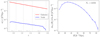 |
Fig. 1. Properties of tracers and voids in the Euclid Flagship mock catalog. Left: number density of spectroscopic galaxies and selected VIDE voids as function of redshift; vertical dashed lines indicate the redshift bins. Right: number density of the same VIDE voids as a function their effective radius R (void size function) from the entire redshift range, encompassing a total of Nv = 44 356 voids with 18.6 h−1 Mpc < R < 84.8 h−1 Mpc. Poisson statistics are assumed for the error bars. We refer to our companion paper for a detailed cosmological forecast based on the void size function (Contarini et al., in prep.). |
4. Data analysis
Our data vector is represented by the void-galaxy cross-correlation function in redshift space. As this function is an-isotropic, we can either consider its 2D version with coordinates perpendicular to and along the line of sight, ξs(s⊥, s∥), or its decomposition into multipoles by use of Legendre polynomials Pℓ of order ℓ,
 (15)
(15)
where μs = s∥/s. We highlight that the notations ξs(s), ξs(s⊥, s∥), and ξs(s, μs) all refer to the same physical quantity, albeit via their different mathematical formulations. Here, we make use of the full 2D correlation function for our model fits, since it contains all the available information on RSD and AP distortions. For the sake of completeness, we additionally provide the three multipoles of the lowest even order, ℓ = 0, 2, 4 (i.e., monopole, quadrupole, and hexadecapole). Their theoretical linear predictions directly follow from Eq. (7):
![Mathematical equation: $$ \begin{aligned} \xi ^s_0(s) = \left({1+\frac{f/b}{3}}\right)\xi (r), \quad \xi ^s_2(s) = \frac{2f/b}{3}[{\xi (r)-\overline{\xi }(r)}], \quad \xi ^s_4(s) = 0. \end{aligned} $$](/articles/aa/full_html/2022/02/aa42073-21/aa42073-21-eq21.gif) (16)
(16)
4.1. Estimator
For our mock measurements of ξs(s⊥, s∥), we utilize the Landy & Szalay (1993) estimator for cross correlations,
 (17)
(17)
where the angled brackets signify normalized pair counts of void-center and galaxy positions in the data (𝒟v, 𝒟g) and corresponding random positions (ℛv, ℛg) in bins of s⊥ and s∥. We chose a fixed binning in units of the effective void radius for each individual void and express all distances in units of R as well. This allows one to coherently capture the characteristic topology of voids from a range of sizes including their boundaries in an ensemble-average sense. The resulting statistic is also referred to as a void stack or stacked void-galaxy cross-correlation function. We have generated the randoms via sampling from the redshift distributions of galaxies and voids as depicted in Fig. 1, but with ten times the number of objects and without spatial clustering. We applied the same angular footprint as for the mock data and additionally assign an effective radius to every void random, drawn from the radius distribution of galaxy voids. The latter is used to express distances from void randoms in units of R, consistent with the stacking procedure of galaxy voids. The uncertainty of the estimated  is quantified by its covariance matrix:
 (18)
(18)
where angled brackets imply averaging over an ensemble of observations. The square root of the diagonal elements,  , are used as error bars on our measurements of
  . Although we can only observe one universe (respectively a single Flagship mock catalog), ergodicity allows us to estimate
  via spatial averaging over distinct patches. This naturally motivates the jackknife technique to be applied on the available sample of voids, which are non-overlapping. Therefore, we simply remove one void at a time in the estimator of ξs from Eq. (17), which provides Nv jackknife samples. This approach has been tested on simulations and validated on mocks in previous analyses (Paz et al. 2013; Cai et al. 2016; Correa et al. 2019; Hamaus et al. 2020). It has further been shown that, in the limit of large sample sizes, the jackknife technique provides consistent covariance estimates compared to the ones obtained from many independent mock catalogs (Favole et al. 2021). Residual differences between the two methods indicate the jackknife approach to yield somewhat higher covariances, which renders our error forecast conservative.
4.2. Model and likelihood
As previously demonstrated in Hamaus et al. (2020), we include two additional nuisance parameters, ℳ and 𝒬, in the theory model of Eq. (7), enabling us to account for systematic effects. Here, ℳ (monopole-like) is used as a free amplitude of the deprojected correlation function ξ(r) in real space and 𝒬 (quadrupole-like) is a free amplitude for the quadrupole term proportional to μ2. Here, we adopt a slightly modified, empirically motivated parametrization of this model, with enhanced coefficients for the Jacobian (second and third) terms in Eq. (19),
![Mathematical equation: $$ \begin{aligned} \xi ^s(s_\perp ,s_\parallel ) = \mathcal{M} \left\{ \xi (r) + \frac{f}{b}\overline{\xi }(r) + 2\mathcal{Q} \,\frac{f}{b}\mu ^2[{\xi (r)-\overline{\xi }(r)}]\right\} . \end{aligned} $$](/articles/aa/full_html/2022/02/aa42073-21/aa42073-21-eq28.gif) (19)
(19)
The parameter ℳ adjusts for potential inaccuracies arising in the deprojection technique and a contamination of the void sample by spurious Poisson fluctuations, which can attenuate the amplitude of the monopole and quadrupole (Cousinou et al. 2019). The parameter 𝒬 accounts for possible selection effects when voids are identified in anisotropic redshift space (Pisani et al. 2015b; Correa et al. 2021, 2022). For example, the occurrence of shell crossing and virialization affects the topology of void boundaries in redshift space (Hahn et al. 2015), resulting in the well-known finger-of-God (FoG) effect (Jackson 1972). In turn, this can enhance the Jacobian terms in Eq. (7), which motivates the empirically determined modification of their coefficients in Eq. (19). A similar result can be achieved by enhancing the values of ℳ and 𝒬, but keeping the original form of Eq. (7), which can be approximately understood as a redefinition of the nuisance parameters. However, the form of Eq. (19) is found to better describe the void-galaxy cross-correlation function in terms of goodness of fit, while at the same time yields nuisance parameters that are distributed more closely around values of one. This approach is akin to other empirical model extensions that have been proposed in the literature (e.g., Achitouv 2017; Paillas et al. 2021).
For the mapping from the observed separations s⊥ and s∥ to r and μ, we use Eq. (3) together with Eq. (10) for the AP effect. This yields the following transformation between coordinates in real and redshift space,
![Mathematical equation: $$ \begin{aligned} r_\perp = q_\perp s_\perp ,\qquad r_\parallel = q_\parallel s_\parallel \left[{1-\frac{1}{3}\frac{f}{b}\mathcal{M} \,\overline{\xi }(r)}\right]^{-1}, \end{aligned} $$](/articles/aa/full_html/2022/02/aa42073-21/aa42073-21-eq29.gif) (20)
(20)
which can be solved via iteration to determine  and μ = r∥/r, starting from an initial value of r = s (Hamaus et al. 2020). In practice, we express all separations in units of the observable effective radius R of each void in redshift space, but noting that the AP effect yields
  in the true cosmology (Hamaus et al. 2020; Correa et al. 2021). When expressing Eq. (20) in units of R*, only ratios of q⊥ and q∥ appear, which defines the AP parameter ε = q⊥/q∥. The latter is particularly well constrained via the AP test from standard spheres (Lavaux & Wandelt 2012; Hamaus et al. 2015).
Finally, given the estimated data vector from Eq. (17), its covariance from Eq. (18), and the model from Eqs. (19) and (20), we can construct a Gaussian likelihood  of the data
  given the model parameter vector Θ = (f/b, ε, ℳ, 𝒬) as:
 (21)
(21)
We apply the factor of Hartlap et al. (2007) to estimate the inverse covariance matrix, which amounts to a correction of at most 3% in our case. Because the model ξs(s|Θ) makes use of the data to calculate ξ(r) via Eq. (5), it contributes its own covariance and becomes correlated with  . However, by treating the amplitude of ξ(r) as the free parameter ℳ in our model, we marginalize over its uncertainty. A correlation between model and data can only act to reduce the total covariance in our likelihood, so the resulting parameter errors can be regarded as upper limits in this respect. Due to their finite size, some voids extend beyond the boundaries of a given bin in redshift, which necessarily results in some degree of correlation between the parameter measurements at adjacent redshift bins. As a boundary effect, we expect this correlation to be small and hence neglect it here.
We use the affine-invariant Markov chain Monte Carlo (MCMC) ensemble sampler emcee (Foreman-Mackey et al. 2019) to sample the posterior probability distribution of all model parameters. The quality of the maximum-likelihood model (best fit) can be assessed via evaluation of the reduced χ2 statistic:
 (22)
(22)
with Nd.o.f. = Nbin − Npar degrees of freedom, where Nbin is the number of bins for the data and Npar the number of model parameters. We use 18 bins per dimension for the 2D void-galaxy cross-correlation function, which yields Nbin = 324. This number is high enough to accurately sample the scale dependence of  , yet significantly smaller than the available number of voids per redshift bin, ensuring sufficient statistics for the estimation of its covariance matrix. With Npar = 4, this implies Nd.o.f. = 320.
4.3. Deprojection and fit
In order to evaluate our model from Eq. (19), we need to obtain the real-space correlation function ξ(r), which can be calculated via an inverse Abel transform of the projected redshift-space correlation function  , following Eq. (5). We estimate the function
  directly via line-of-sight integration of
  , as in the first equality of Eq. (6), and use a cubic spline to interpolate both
  and ξ(r). The results are presented in Fig. 2 for each of our four redshift bins. Thanks to the large number of voids in each bin, the statistical noise is low and enables a smooth deprojection of the data. Some residual noise can be noted at the innermost bins, namely, for small separations from the void center, which causes the deprojection and the subsequent spline interpolation to be less accurate (Pisani et al. 2014; Hamaus et al. 2020). For this reason, we omit the first radial bin of the data in our model fits below, but we checked that even discarding the central three bins of s, s⊥, and s∥ in our analysis yields consistent results. From the full Euclid footprint of about three times the size of an octant, the residual statistical noise of this procedure will be reduced further, so our mock analysis can be considered conservative in this regard.
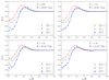 |
Fig. 2. Projected void-galaxy cross-correlation function |


We also plot the monopole of the redshift-space correlation function, which nicely follows the shape of the deprojected ξ(r), as expected from Eq. (16). Moreover, our model from Eqs. (19) and (20) provides a very accurate fit to this monopole everywhere apart from its innermost bins, implying that any residual errors in the model remain negligibly small in that regime. We notice an increasing amplitude of all correlation functions towards lower redshift, partly reflecting the growth of overdensities along the void walls, while their interior is gradually evacuated. The increase in mean effective radius with redshift is not of dynamical origin, it is a consequence of the declining galaxy density ng(z), see Fig. 1. A higher space density of tracers enables the identification of smaller voids.
We minimize the log-likelihood of Eq. (21) by varying the model parameters to find the best-fit model to the mock data. As a data vector, we used the 2D void-galaxy cross-correlation  , which contains the complete information on dynamic and geometric distortions from all multipole orders. However, we checked that our pipeline yields consistent constraints when only considering the three lowest even multipoles,
  , of order ℓ = 0, 2, 4 as our data vector. The results are shown in Fig. 3 for our four consecutive redshift bins. In each case, we find extraordinary agreement between the model and the data, which is further quantified by the reduced χ2 being so close to unity in all bins. Again, it is possible to perceive the slight deepening of voids over time and the agglomeration of matter in their surroundings. The multipoles shown in the right column of Fig. 3 complement this view, with both monopole and quadrupole enhancing their amplitudes during void evolution, and they exhibit an excellent agreement with the model. The quadrupole vanishes towards the central void region and the model mismatch in the first few bins of the monopole has negligible impact here, as most of the anisotropic information originates from larger scales. In addition, the hexadecapole remains consistent with zero at all times, in accordance with Eq. (16).
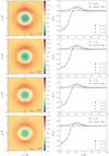 |
Fig. 3. Stacked void-galaxy cross-correlation function in redshift space. Left: ξs(s⊥, s∥) in 2D (color scale with black contours) and its best-fit model from Eqs. (19) and (20) (white contours). Right: monopole (blue dots), quadrupole (red triangles) and hexadecapole (green wedges) of ξs(s⊥, s∥) and best-fit model (solid, dashed, dotted lines). The mean void redshift, |


4.4. Parameter constraints
Performing a full MCMC run for each redshift bin, we obtain the posteriors for our model parameters as shown in Fig. 4. We observe a similar correlation structure as in the previous BOSS analysis of Hamaus et al. (2020). Namely, a weak correlation between f/b and ε, and a strong anti-correlation between f/b and ℳ. Overall, the 68% confidence regions for f/b and ε agree well with the expected input values, shown as dashed lines. In a ΛCDM cosmology, the linear growth rate is given by
![Mathematical equation: $$ \begin{aligned} f(z)\simeq \left[{\frac{\Omega _{\rm m}(1+z)^3}{H^2(z)/H_0^2}}\right]^{\,\gamma }, \end{aligned} $$](/articles/aa/full_html/2022/02/aa42073-21/aa42073-21-eq50.gif) (23)
(23)
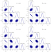 |
Fig. 4. Posterior probability distribution of the model parameters that enter in Eqs. (19) and (20), obtained via MCMC from the data shown in the left of Fig. 3. Dark and light shaded areas represent 68% and 95% confidence regions with a cross marking the best fit, dashed lines indicate fiducial values of the RSD and AP parameters. The top of each column states the mean and standard deviation of the 1D marginal distributions. Adjacent bins in void redshift with mean value |

with a growth index of γ ≃ 0.55 (Lahav et al. 1991; Linder 2005). We take the Flagship measurements of the large-scale linear bias b from our companion paper (Contarini et al., in prep.), which uses CAMB (Lewis et al. 2000) to calculate the dark-matter correlation function to compare with the estimated galaxy auto-correlation function (see Marulli et al. 2013, 2018, for details). As we are using the correct input cosmology of Flagship to convert angles and redshifts to comoving distances following Eq. (9), we have ε = 1 as fiducial value.
For the values of the nuisance parameters, ℳ and 𝒬, we do not have any specific expectation, but we set their defaults to unity as well. We also find their posteriors to be distributed around values of one, although their mean can deviate more than one standard deviation from that default value. However, the distributions of the nuisance parameters are not relevant for the cosmological interpretation of the posterior, as they can be marginalized over. The relative precision on f/b ranges between 7.3% and 8.0%, while the one on ε is between 0.87% and 0.91%. This precision corresponds to a survey area of one octant of the sky, but the footprint covered by Euclid will be roughly three times as large. Therefore, one can expect these numbers to decrease by a factor of  to yield about 4% accuracy on f/b and 0.5% on ε per redshift bin.
The attainable precision can even further be increased via a calibration strategy. Hamaus et al. (2020) have shown that this is possible when the model ingredients ξ(r), ℳ, and 𝒬 are taken from external sources, instead of being constrained by the data itself, for example, from a large number of high-fidelity survey mocks. However, we emphasize that this practice introduces a prior dependence on the assumed model parameters in the mocks, so it underestimates the final uncertainty on cosmology and may yield biased results. We also note that survey mocks are typically designed to reproduce the two-point statistics of galaxies on large scales, but are not guaranteed to provide void statistics at a similar level of accuracy.
Nevertheless, for the sake of completeness we investigate the achievable precision when fixing the nuisance parameters to their best-fit values in the full analysis, while still inferring ξ(r) via deprojection of the data as before. We note that this is an arbitrary choice of calibration, in practice, the values of ℳ and 𝒬 will depend on the type of mocks considered. The resulting posteriors on f/b and ε are shown in Fig. 5. The calibrated analysis yields a relative precision of 1.3% to 1.8% on f/b and 0.72% to 0.75% on ε. Compared to the calibration-independent analysis, this amounts to an improvement by up to a factor of about 5 for constraints on f/b and 1.2 for ε. Extrapolated to the full survey area accessible to Euclid, this corresponds to a precision of roughly 1% on f/b and 0.4% on ε per redshift bin. As expected, these calibrated constraints are more prone to be biased with respect to the underlying cosmology, as evident from Fig. 5 given our choice of calibration. It is also interesting to note that f/b and ε are less correlated in the calibrated analysis, since their partial degeneracy with the nuisance parameter ℳ is removed.
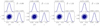 |
Fig. 5. Posterior probability distribution of the model parameters that enter in Eqs. (19) and (20). Details are the same as in Fig. 4, but with a fixing (calibration) of the nuisance parameters ℳ and 𝒬 to their best-fit values. Redshift increases from left to right, as indicated. |
We summarize all of our results in Table 1. The constraints on fσ8 and DMH are derived from the posteriors on f/b and ε. In the former case, we assume ξ(r)∝bσ8 and, hence, we multiply f/b by the underlying value of bσ8 in the Flagship mock, which also assumes the relative precision on f/b and fσ8 to be the same. Moreover, we neglect the dependence on h that enters in the definition of σ8 and should be marginalized over (Sánchez 2020). For the latter case, we multiply ε by the fiducial DMH, following Eq. (11). The results on fσ8 and DMH from both model-independent and calibrated analyses are also shown in Fig. 6.
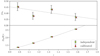 |
Fig. 6. Measurement of fσ8 and DMH from VIDE voids in the Euclid Flagship catalog as a function of redshift z. The marker style distinguishes between a fully model-independent approach (green circles) and an analysis with calibrated nuisance parameters ℳ and 𝒬 (red triangles) using external sources, such as simulations or mocks. Dotted lines indicate the Flagship input cosmology, the markers are slightly shifted horizontally for visibility. These results are based on one octant of the sky, the expected precision from the full Euclid footprint is a factor of about |

RSD and AP parameter constraints.
5. Discussion
The measurements of fσ8 and DMH as a function of redshift can be used to constrain cosmological models. For example, an inversion of Eq. (12) provides ΩΛ = 1 − Ωm, the only free parameter of the product DMH in a flat ΛCDM cosmology. Using our Flagship mock measurements of DMH we sample the joint posterior on ΩΛ from all of our redshift bins combined. Considering the full Euclid footprint to be approximately three times the size of our Flagship mock catalog, we scale the errors on DMH by a factor of  and center its mean values to the input cosmology of Flagship. The resulting posterior yields ΩΛ = 0.6809 ± 0.0048, in the model-independent, and ΩΛ = 0.6810 ± 0.0039, in the calibrated case from the analysis of Euclid voids alone. The corresponding result obtained by Planck in 2018 (Planck Collaboration VI 2020) is ΩΛ = 0.6847 ± 0.0073, including cosmic microwave background (CMB) lensing and ΩΛ = 0.6889 ± 0.0056, when combined with BOSS BAO data (Alam et al. 2017). The main cosmological probes of Euclid, when altogether combined, are forecasted to achieve a 1σ uncertainty of 0.0071 on ΩΛ in a pessimistic scenario and 0.0025 in an optimistic case (Euclid Collaboration 2020). The expected precision on ΩΛ from the analysis of Euclid voids alone will hence likely match the level of precision from Planck and the combined main Euclid probes. The left panel of Fig. 7 provides a visual comparison of the constraining power on ΩΛ from the mentioned experiments, including the one previously obtained from BOSS voids in Hamaus et al. (2020).
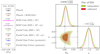 |
Fig. 7. Forecast for cosmological constraints on dark energy parameters. Left: comparison of the constraining power on ΩΛ in a flat ΛCDM cosmology from Planck 2018 alone (Planck Collaboration VI 2020) and when combined with BOSS BAO data (Alam et al. 2017). Below, constraints as obtained with BOSS voids via RSD and AP (Hamaus et al. 2020), as expected from Euclid voids (this work), and as expected from Euclid’s main cosmological probes combined (Euclid Collaboration 2020). Calibrated constraints from voids are indicated by the abbreviation “cal.” and the Euclid main probes distinguish between “optimistic” and “pessimistic” scenarios. Right: predicted constraints from Euclid voids on dark energy content Ωde and its equation-of-state parameter w in a flat wCDM cosmology. Both the model-independent (green) and the calibrated results (red) are shown, dashed lines indicate the input cosmology. Mean parameter values and their 68% confidence intervals for the model-independent case are shown at the top of each panel. |
Furthermore, in Euclid we aim to explore cosmological models beyond ΛCDM. One minimal extension is to replace the cosmological constant, Λ, by a more general form of dark energy with density Ωde, and a constant equation-of-state parameter, w. This modifies the Hubble function in Eq. (12) to
 (24)
(24)
which reduces to the case of flat ΛCDM for w = −1. Using our rescaled and recentered mock measurements of DMH, we can thus infer the posterior distribution of the parameter pair (Ωde, w). The result is shown in the right panel of Fig. 7 for both the model-independent and the calibrated analysis, assuming flat priors with Ωde ∈ [0, 1] and w ∈ [−10, 10]. We observe a mild degeneracy between Ωde and w, which can be mitigated in the calibrated case. However, this may come at the price of an increased bias from the true cosmology. Nevertheless, these parameter constraints are extremely competitive, yielding  and, hence, a relative precision of about 9% in the calibrated scenario. In the model-independent analysis, we still obtain
  with a relative precision of 11%. The constraints on Ωde are similar to the ones on ΩΛ from above. We note that this result is in remarkable agreement with the early Fisher forecast of Lavaux & Wandelt (2012), corroborating the robustness of the AP test with voids. The Planck Collaboration VI (2020) obtain
  including CMB lensing in the same wCDM model and a combination with BAO yields a similar precision of about 10%, with
  .
.
The right panel of Fig. 7 provides a demonstration of how cosmic voids by themselves constrain the properties of dark energy, without the inclusion of external priors, observables, or mock data. A combination with other probes, such as void abundance (Contarini et al., in prep.), cluster abundance (Sahlén 2019), BAO (Nadathur et al. 2019), CMB, or weak lensing (Bonici et al., in prep.) will, of course, provide substantial gains. This is particularly relevant when extended cosmological models are considered to enable the breaking of parameter degeneracies. For example, it concerns models with a redshift-dependent equation of state w(z), nonzero curvature, or massive neutrinos. In those cases, however, the calibrated approach is prone to be biased towards the fiducial cosmology adopted in the synthetic mock data used for calibration, which commonly assumes a flat ΛCDM model. In order to avoid the emergence of confirmation bias, we advocate the more conservative model-independent approach, even if it comes at the price of a somewhat reduced statistical precision.
In our analysis, we have neglected observational systematics that are expected to arise in Euclid data, such as spectral line misidentification due to interlopers that can lead to catastrophic redshift errors (Pullen et al. 2016; Leung et al. 2017; Massara et al. 2021). However, this effect mainly impacts the amplitude of multipoles (Addison et al. 2019; Grasshorn Gebhardt et al. 2019), so we anticipate it to be at least partially captured by the nuisance parameters in our model. We leave a more detailed investigation on the impact of survey systematics to a future work.
6. Conclusion
In this work, we investigate the prospects for performing a cosmological analysis using voids extracted from the spectroscopic galaxy sample of the Euclid Survey. The method we applied is based on the observable distortions of average void shapes via RSD and the AP effect. Our forecast relies on one light cone octant (5157 deg2) of the Flagship simulation covering a redshift range of 0.9 < z < 1.8, which provides the most realistic mock galaxy catalog available for this purpose to date. Exploiting a deprojection technique and assuming linear mass conservation allows us to accurately model the anisotropic void-galaxy cross-correlation function in redshift space. We explore the likelihood of the mock data given this model via MCMCs and obtain the posterior distributions for our model parameters: the ratio of growth rate and bias f/b, and the geometric AP distortion ε. Two additional nuisance parameters, ℳ and 𝒬, are used to account for systematic effects in the data; they can either be marginalized over (model-independent approach) or calibrated via external sources, such as survey mocks (calibrated approach). After the conversion of our model parameters to the combinations fσ8 and DMH, we forecast the attainable precision of their measurement with voids in Euclid.
We expect a relative precision of about 4% (1%) on fσ8 and 0.5% (0.4%) on DMH without (with) model calibration for each of our four redshift bins. This level of precision will enable very competitive constraints on cosmological parameters. For example, it yields a 0.7% (0.6%) constraint on ΩΛ in a flat ΛCDM cosmology and a 11% (9%) constraint on the equation-of-state parameter w for dark energy in wCDM from the AP test with voids alone. A combination with other void statistics, or the main cosmological probes of Euclid, such as galaxy clustering and weak lensing, will enable considerable improvements in accuracy and allow for the exploration of a broader range of extended cosmological models with a larger scope of parameters.
Acknowledgments
NH, GP and JW are supported by the Excellence Cluster ORIGINS, which is funded by the Deutsche Forschungsgemeinschaft (DFG, German Research Foundation) under Germany’s Excellence Strategy – EXC-2094 – 390783311. MA, MCC and SE are supported by the eBOSS ANR grant (under contract ANR-16-CE31-0021) of the French National Research Agency, the OCEVU LABEX (Grant No. ANR-11-LABX-0060) and the A*MIDEX project (Grant No. ANR-11-IDEX-0001-02) funded by the Investissements d’Avenir French government program, and by CNES, the French National Space Agency. AP is supported by NASA ROSES grant 12-EUCLID12-0004, and NASA grant 15-WFIRST15-0008 to the Nancy Grace Roman Space Telescope Science Investigation Team “Cosmology with the High Latitude Survey”. GL is supported by the ANR BIG4 project, grant ANR-16-CE23-0002 of the French Agence Nationale de la Recherche. PN is funded by the Centre National d’Etudes Spatiales (CNES). We acknowledge use of the Python libraries NumPy (Harris et al. 2020), SciPy (Virtanen et al. 2020), Matplotlib (Hunter 2007), Astropy (Astropy Collaboration 2013, 2018), emcee (Foreman-Mackey et al. 2019), GetDist (Lewis 2019), healpy (Górski et al. 2005; Zonca et al. 2019), and PyAbel (Hickstein et al. 2019). This work has made use of CosmoHub (Carretero et al. 2017; Tallada et al. 2020). CosmoHub has been developed by the Port d’Informació Científica (PIC), maintained through a collaboration of the Institut de Física d’Altes Energies (IFAE) and the Centro de Investigaciones Energéticas, Medioambientales y Tecnológicas (CIEMAT) and the Institute of Space Sciences (CSIC & IEEC), and was partially funded by the “Plan Estatal de Investigación Científica y Técnica y de Innovación” program of the Spanish government. The Euclid Consortium acknowledges the European Space Agency and a number of agencies and institutes that have supported the development of Euclid, in particular the Academy of Finland, the Agenzia Spaziale Italiana, the Belgian Science Policy, the Canadian Euclid Consortium, the Centre National d’Etudes Spatiales, the Deutsches Zentrum für Luft- und Raumfahrt, the Danish Space Research Institute, the Fundação para a Ciência e a Tecnologia, the Ministerio de Economia y Competitividad, the National Aeronautics and Space Administration, the Netherlandse Onderzoekschool Voor Astronomie, the Norwegian Space Agency, the Romanian Space Agency, the State Secretariat for Education, Research and Innovation (SERI) at the Swiss Space Office (SSO), and the United Kingdom Space Agency. A complete and detailed list is available on the Euclid website (http://www.euclid-ec.org).
References
- Abel, N. H. 1842, in Oeuvres Completes, eds. L. Sylow, & S. Lie (New York: Johnson Reprint Corp.), 27 [Google Scholar]
- Abel, T., Hahn, O., & Kaehler, R. 2012, MNRAS, 427, 61 [Google Scholar]
- Achitouv, I. 2016, Phys. Rev. D, 94, 103524 [NASA ADS] [CrossRef] [Google Scholar]
- Achitouv, I. 2017, Phys. Rev. D, 96, 083506 [NASA ADS] [CrossRef] [Google Scholar]
- Achitouv, I. 2019, Phys. Rev. D, 100, 123513 [NASA ADS] [CrossRef] [Google Scholar]
- Addison, G. E., Bennett, C. L., Jeong, D., Komatsu, E., & Weiland, J. L. 2019, ApJ, 879, 15 [NASA ADS] [CrossRef] [Google Scholar]
- Alam, S., Ata, M., Bailey, S., et al. 2017, MNRAS, 470, 2617 [Google Scholar]
- Alam, S., Aubert, M., Avila, S., et al. 2021a, Phys. Rev. D, 103, 083533 [NASA ADS] [CrossRef] [Google Scholar]
- Alam, S., Aviles, A., Bean, R., et al. 2021b, JCAP, 11, 050 [Google Scholar]
- Albrecht, A., Bernstein, G., Cahn, R., et al. 2006, ArXiv e-prints [arXiv:astro-ph/0609591] [Google Scholar]
- Alcock, C., & Paczynski, B. 1979, Nature, 281, 358 [NASA ADS] [CrossRef] [Google Scholar]
- Alonso, D., Hill, J. C., Hložek, R., & Spergel, D. N. 2018, Phys. Rev. D, 97, 063514 [NASA ADS] [CrossRef] [Google Scholar]
- Amendola, L., Appleby, S., Avgoustidis, A., et al. 2018, Liv. Rev. Relativ., 21, 2 [NASA ADS] [CrossRef] [Google Scholar]
- Astropy Collaboration (Robitaille, T. P., et al.) 2013, A&A, 558, A33 [NASA ADS] [CrossRef] [EDP Sciences] [Google Scholar]
- Astropy Collaboration (Price-Whelan, A. M., et al.) 2018, AJ, 156, 123 [Google Scholar]
- Aubert, M., Cousinou, M.-C., Escoffier, S., et al. 2020, ArXiv e-prints [arXiv:2007.09013] [Google Scholar]
- Baker, T., Clampitt, J., Jain, B., & Trodden, M. 2018, Phys. Rev. D, 98, 023511 [NASA ADS] [CrossRef] [Google Scholar]
- Baldi, M., & Villaescusa-Navarro, F. 2018, MNRAS, 473, 3226 [NASA ADS] [CrossRef] [Google Scholar]
- Banerjee, A., & Dalal, N. 2016, JCAP, 11, 015 [CrossRef] [Google Scholar]
- Barreira, A., Cautun, M., Li, B., Baugh, C. M., & Pascoli, S. 2015, JCAP, 2015, 028 [Google Scholar]
- Bayer, A. E., Villaescusa-Navarro, F., Massara, E., et al. 2021, ApJ, 919, 24 [NASA ADS] [CrossRef] [Google Scholar]
- Behroozi, P. S., Wechsler, R. H., & Wu, H.-Y. 2013, ApJ, 762, 109 [NASA ADS] [CrossRef] [Google Scholar]
- Bertschinger, E. 1985, ApJS, 58, 1 [NASA ADS] [CrossRef] [Google Scholar]
- Blanton, M. R., Hogg, D. W., Bahcall, N. A., et al. 2003, ApJ, 592, 819 [Google Scholar]
- Blanton, M. R., Lupton, R. H., Schlegel, D. J., et al. 2005, ApJ, 631, 208 [Google Scholar]
- Bos, E. G. P., van de Weygaert, R., Dolag, K., & Pettorino, V. 2012, MNRAS, 426, 440 [NASA ADS] [CrossRef] [Google Scholar]
- Bracewell, R. 1999, The Fourier Transform and its Applications, 3rd edn. (New York: McGraw-Hill), 262 [Google Scholar]
- Brouwer, M. M., Demchenko, V., Harnois-Déraps, J., et al. 2018, MNRAS, 481, 5189 [NASA ADS] [CrossRef] [Google Scholar]
- Cai, Y.-C., Cole, S., Jenkins, A., & Frenk, C. S. 2010, MNRAS, 407, 201 [NASA ADS] [CrossRef] [Google Scholar]
- Cai, Y.-C., Neyrinck, M. C., Szapudi, I., Cole, S., & Frenk, C. S. 2014, ApJ, 786, 110 [NASA ADS] [CrossRef] [Google Scholar]
- Cai, Y.-C., Padilla, N., & Li, B. 2015, MNRAS, 451, 1036 [NASA ADS] [CrossRef] [Google Scholar]
- Cai, Y.-C., Taylor, A., Peacock, J. A., & Padilla, N. 2016, MNRAS, 462, 2465 [NASA ADS] [CrossRef] [Google Scholar]
- Cai, Y.-C., Neyrinck, M., Mao, Q., et al. 2017, MNRAS, 466, 3364 [NASA ADS] [CrossRef] [Google Scholar]
- Carretero, J., Castander, F. J., Gaztañaga, E., Crocce, M., & Fosalba, P. 2015, MNRAS, 447, 646 [NASA ADS] [CrossRef] [Google Scholar]
- Carretero, J., Tallada, P., Casals, J., et al. 2017, Proceedings of the European Physical Society Conference on High Energy Physics, 5–12 July, 488 [CrossRef] [Google Scholar]
- Chan, K. C., & Hamaus, N. 2021, Phys. Rev. D, 103, 043502 [NASA ADS] [CrossRef] [Google Scholar]
- Chan, K. C., Hamaus, N., & Desjacques, V. 2014, Phys. Rev. D, 90, 103521 [NASA ADS] [CrossRef] [Google Scholar]
- Chan, K. C., Hamaus, N., & Biagetti, M. 2019, Phys. Rev. D, 99, 121304 [CrossRef] [Google Scholar]
- Chantavat, T., Sawangwit, U., & Wandelt, B. D. 2017, ApJ, 836, 156 [NASA ADS] [CrossRef] [Google Scholar]
- Clampitt, J., & Jain, B. 2015, MNRAS, 454, 3357 [NASA ADS] [CrossRef] [Google Scholar]
- Clampitt, J., Cai, Y.-C., & Li, B. 2013, MNRAS, 431, 749 [NASA ADS] [CrossRef] [Google Scholar]
- Contarini, S., Ronconi, T., Marulli, F., et al. 2019, MNRAS, 488, 3526 [NASA ADS] [CrossRef] [Google Scholar]
- Contarini, S., Marulli, F., Moscardini, L., et al. 2021, MNRAS, 504, 5021 [NASA ADS] [CrossRef] [Google Scholar]
- Correa, C. M., Paz, D. J., Padilla, N. D., et al. 2019, MNRAS, 485, 5761 [NASA ADS] [CrossRef] [Google Scholar]
- Correa, C. M., Paz, D. J., Sánchez, A. G., et al. 2021, MNRAS, 500, 911 [Google Scholar]
- Correa, C. M., Paz, D. J., Padilla, N. D., et al. 2022, MNRAS, 509, 1871 [Google Scholar]
- Costille, A., Caillat, A., Rossin, C., et al. 2018, SPIE Conf. Ser., 10698, 106982B [Google Scholar]
- Cousinou, M. C., Pisani, A., Tilquin, A., et al. 2019, Astron. Comput., 27, 53 [NASA ADS] [CrossRef] [Google Scholar]
- Crocce, M., Castander, F. J., Gaztañaga, E., Fosalba, P., & Carretero, J. 2015, MNRAS, 453, 1513 [NASA ADS] [CrossRef] [Google Scholar]
- Cropper, M., Pottinger, S., Azzollini, R., et al. 2018, SPIE Conf. Ser., 10698, 1069828 [NASA ADS] [Google Scholar]
- Davies, C. T., Cautun, M., & Li, B. 2019, MNRAS, 490, 4907 [NASA ADS] [CrossRef] [Google Scholar]
- Dawson, K. S., Schlegel, D. J., Ahn, C. P., et al. 2013, AJ, 145, 10 [Google Scholar]
- Dawson, K. S., Kneib, J.-P., Percival, W. J., et al. 2016, AJ, 151, 44 [Google Scholar]
- de Jong, J. T. A., Verdoes Kleijn, G. A., Kuijken, K. H., & Valentijn, E. A. 2013, Exp. Astron., 35, 25 [Google Scholar]
- Dolag, K., Komatsu, E., & Sunyaev, R. 2016, MNRAS, 463, 1797 [Google Scholar]
- Eisenstein, D. J., Weinberg, D. H., Agol, E., et al. 2011, AJ, 142, 72 [Google Scholar]
- Euclid Collaboration (Blanchard, A., et al.) 2020, A&A, 642, A191 [NASA ADS] [CrossRef] [EDP Sciences] [Google Scholar]
- Falck, B., Koyama, K., Zhao, G.-B., & Cautun, M. 2018, MNRAS, 475, 3262 [NASA ADS] [CrossRef] [Google Scholar]
- Fang, Y., Hamaus, N., Jain, B., et al. 2019, MNRAS, 490, 3573 [NASA ADS] [CrossRef] [Google Scholar]
- Favole, G., Granett, B. R., Silva Lafaurie, J., & Sapone, D. 2021, MNRAS, 505, 5833 [NASA ADS] [CrossRef] [Google Scholar]
- Foreman-Mackey, D., Farr, W., Sinha, M., et al. 2019, J. Open Sour. Softw., 4, 1864 [Google Scholar]
- Forero-Sánchez, D., Zhao, C., Tao, C., et al. 2021, MNRAS, submitted [arXiv:2107.02950] [Google Scholar]
- Gonçalves, R. S., Carvalho, G. C., Andrade, U., et al. 2021, JCAP, 2021, 029 [CrossRef] [Google Scholar]
- Górski, K. M., Hivon, E., Banday, A. J., et al. 2005, ApJ, 622, 759 [Google Scholar]
- Granett, B. R., Neyrinck, M. C., & Szapudi, I. 2008, ApJ, 683, L99 [NASA ADS] [CrossRef] [Google Scholar]
- Grasshorn Gebhardt, H. S., Jeong, D., Awan, H., et al. 2019, ApJ, 876, 32 [NASA ADS] [CrossRef] [Google Scholar]
- Gregory, S. A., & Thompson, L. A. 1978, ApJ, 222, 784 [NASA ADS] [CrossRef] [Google Scholar]
- Gruen, D., Friedrich, O., Amara, A., et al. 2016, MNRAS, 455, 3367 [Google Scholar]
- Guzzo, L., Scodeggio, M., Garilli, B., et al. 2014, A&A, 566, A108 [NASA ADS] [CrossRef] [EDP Sciences] [Google Scholar]
- Habouzit, M., Pisani, A., Goulding, A., et al. 2020, MNRAS, 493, 899 [NASA ADS] [CrossRef] [Google Scholar]
- Hahn, O., Porciani, C., Carollo, C. M., & Dekel, A. 2007, MNRAS, 375, 489 [NASA ADS] [CrossRef] [Google Scholar]
- Hahn, O., Angulo, R. E., & Abel, T. 2015, MNRAS, 454, 3920 [Google Scholar]
- Hamaus, N., Wandelt, B. D., Sutter, P. M., Lavaux, G., & Warren, M. S. 2014a, Phys. Rev. Lett., 112, 041304 [NASA ADS] [CrossRef] [Google Scholar]
- Hamaus, N., Sutter, P. M., Lavaux, G., & Wandelt, B. D. 2014b, JCAP, 12, 013 [Google Scholar]
- Hamaus, N., Sutter, P. M., & Wandelt, B. D. 2014c, Phys. Rev. Lett., 112, 251302 [NASA ADS] [CrossRef] [Google Scholar]
- Hamaus, N., Sutter, P. M., Lavaux, G., & Wandelt, B. D. 2015, JCAP, 11, 036 [Google Scholar]
- Hamaus, N., Pisani, A., Sutter, P. M., et al. 2016, Phys. Rev. Lett., 117, 091302 [NASA ADS] [CrossRef] [Google Scholar]
- Hamaus, N., Cousinou, M.-C., Pisani, A., et al. 2017, JCAP, 7, 014 [Google Scholar]
- Hamaus, N., Pisani, A., Choi, J.-A., et al. 2020, JCAP, 2020, 023 [Google Scholar]
- Harris, C. R., Millman, K. J., van der Walt, S. J., et al. 2020, Nature, 585, 357 [NASA ADS] [CrossRef] [Google Scholar]
- Hartlap, J., Simon, P., & Schneider, P. 2007, A&A, 464, 399 [NASA ADS] [CrossRef] [EDP Sciences] [Google Scholar]
- Hawken, A. J., Granett, B. R., Iovino, A., et al. 2017, A&A, 607, A54 [NASA ADS] [CrossRef] [EDP Sciences] [Google Scholar]
- Hawken, A. J., Aubert, M., Pisani, A., et al. 2020, JCAP, 2020, 012 [CrossRef] [Google Scholar]
- Hickstein, D. D., Gibson, S. T., Yurchak, R., Das, D. D., & Ryazanov, M. 2019, Rev. Sci. Instrum., 90, 065115 [NASA ADS] [CrossRef] [Google Scholar]
- Hoyle, F., Rojas, R. R., Vogeley, M. S., & Brinkmann, J. 2005, ApJ, 620, 618 [NASA ADS] [CrossRef] [Google Scholar]
- Hunter, J. D. 2007, Comput. Sci. Eng., 9, 90 [NASA ADS] [CrossRef] [Google Scholar]
- Ilić, S., Langer, M., & Douspis, M. 2013, A&A, 556, A51 [NASA ADS] [CrossRef] [EDP Sciences] [Google Scholar]
- Jõeveer, M., Einasto, J., & Tago, E. 1978, MNRAS, 185, 357 [Google Scholar]
- Jackson, J. C. 1972, MNRAS, 156, 1P [CrossRef] [Google Scholar]
- Jennings, E., Li, Y., & Hu, W. 2013, MNRAS, 434, 2167 [CrossRef] [Google Scholar]
- Jones, D. H., Saunders, W., Colless, M., et al. 2004, MNRAS, 355, 747 [NASA ADS] [CrossRef] [Google Scholar]
- Kaiser, N. 1987, MNRAS, 227, 1 [Google Scholar]
- Kirshner, R. P., Oemler, A., Jr., Schechter, P. L., & Shectman, S. A. 1981, ApJ, 248, L57 [NASA ADS] [CrossRef] [Google Scholar]
- Kitaura, F.-S., Chuang, C.-H., Liang, Y., et al. 2016, Phys. Rev. Lett., 116, 171301 [NASA ADS] [CrossRef] [Google Scholar]
- Kovács, A., & García-Bellido, J. 2016, MNRAS, 462, 1882 [Google Scholar]
- Kovács, A., Sánchez, C., García-Bellido, J., et al. 2019, MNRAS, 484, 5267 [CrossRef] [Google Scholar]
- Kreckel, K., Platen, E., Aragón-Calvo, M. A., et al. 2012, AJ, 144, 16 [Google Scholar]
- Kreisch, C. D., Pisani, A., Carbone, C., et al. 2019, MNRAS, 488, 4413 [NASA ADS] [CrossRef] [Google Scholar]
- Kreisch, C. D., Pisani, A., Villaescusa-Navarro, F., et al. 2021, ApJ, submitted [arXiv:2107.02304] [Google Scholar]
- Lahav, O., Lilje, P. B., Primack, J. R., & Rees, M. J. 1991, MNRAS, 251, 128 [Google Scholar]
- Landy, S. D., & Szalay, A. S. 1993, ApJ, 412, 64 [Google Scholar]
- Laureijs, R., Amiaux, J., Arduini, S., et al. 2011, ArXiv e-prints [arXiv:1110.3193] [Google Scholar]
- Laurent, P., Le Goff, J.-M., Burtin, E., et al. 2016, JCAP, 2016, 060 [CrossRef] [Google Scholar]
- Lavaux, G., & Wandelt, B. D. 2012, ApJ, 754, 109 [NASA ADS] [CrossRef] [Google Scholar]
- Leclercq, F., Jasche, J., Sutter, P. M., Hamaus, N., & Wandelt, B. 2015, JCAP, 3, 047 [Google Scholar]
- Lee, J., & Park, D. 2009, ApJ, 696, L10 [NASA ADS] [CrossRef] [Google Scholar]
- Leung, A. S., Acquaviva, V., Gawiser, E., et al. 2017, ApJ, 843, 130 [NASA ADS] [CrossRef] [Google Scholar]
- Lewis, A. 2019, ArXiv e-prints [arXiv:1910.13970] [Google Scholar]
- Lewis, A., Challinor, A., & Lasenby, A. 2000, ApJ, 538, 473 [Google Scholar]
- Liang, Y., Zhao, C., Chuang, C.-H., Kitaura, F.-S., & Tao, C. 2016, MNRAS, 459, 4020 [NASA ADS] [CrossRef] [Google Scholar]
- Linder, E. V. 2005, Phys. Rev. D, 72, 043529 [Google Scholar]
- Mao, Q., Berlind, A. A., Scherrer, R. J., et al. 2017, ApJ, 835, 160 [NASA ADS] [CrossRef] [Google Scholar]
- Marulli, F., Bolzonella, M., Branchini, E., et al. 2013, A&A, 557, A17 [NASA ADS] [CrossRef] [EDP Sciences] [Google Scholar]
- Marulli, F., Veropalumbo, A., Sereno, M., et al. 2018, A&A, 620, A1 [NASA ADS] [CrossRef] [EDP Sciences] [Google Scholar]
- Massara, E., Villaescusa-Navarro, F., Viel, M., & Sutter, P. M. 2015, JCAP, 11, 018 [Google Scholar]
- Massara, E., Ho, S., Hirata, C. M., et al. 2021, MNRAS, 508, 4193 [NASA ADS] [CrossRef] [Google Scholar]
- Melchior, P., Sutter, P. M., Sheldon, E. S., Krause, E., & Wandelt, B. D. 2014, MNRAS, 440, 2922 [NASA ADS] [CrossRef] [Google Scholar]
- Nadathur, S., & Crittenden, R. 2016, ApJ, 830, L19 [CrossRef] [Google Scholar]
- Nadathur, S., Carter, P. M., Percival, W. J., Winther, H. A., & Bautista, J. E. 2019, Phys. Rev. D, 100, 023504 [CrossRef] [Google Scholar]
- Nadathur, S., Woodfinden, A., Percival, W. J., et al. 2020, MNRAS, 499, 4140 [NASA ADS] [CrossRef] [Google Scholar]
- Neyrinck, M. C. 2008, MNRAS, 386, 2101 [CrossRef] [Google Scholar]
- Ntelis, P., Hamilton, J.-C., Le Goff, J.-M., et al. 2017, JCAP, 2017, 019 [CrossRef] [Google Scholar]
- Paillas, E., Cautun, M., Li, B., et al. 2019, MNRAS, 484, 1149 [NASA ADS] [CrossRef] [Google Scholar]
- Paillas, E., Cai, Y.-C., Padilla, N., & Sánchez, A. G. 2021, MNRAS, 505, 5731 [NASA ADS] [CrossRef] [Google Scholar]
- Pan, D. C., Vogeley, M. S., Hoyle, F., Choi, Y.-Y., & Park, C. 2012, MNRAS, 421, 926 [NASA ADS] [CrossRef] [Google Scholar]
- Panchal, R. R., Pisani, A., & Spergel, D. N. 2020, ApJ, 901, 87 [NASA ADS] [CrossRef] [Google Scholar]
- Patiri, S. G., Prada, F., Holtzman, J., Klypin, A., & Betancort-Rijo, J. 2006, MNRAS, 372, 1710 [NASA ADS] [CrossRef] [Google Scholar]
- Paz, D., Lares, M., Ceccarelli, L., Padilla, N., & Lambas, D. G. 2013, MNRAS, 436, 3480 [NASA ADS] [CrossRef] [Google Scholar]
- Peebles, P. J. E. 1980, The Large-Scale Structure of the Universe (Princeton: Princeton University Press) [Google Scholar]
- Peebles, P. J. E. 2001, ApJ, 557, 495 [NASA ADS] [CrossRef] [Google Scholar]
- Perico, E. L. D., Voivodic, R., Lima, M., & Mota, D. F. 2019, A&A, 632, A52 [NASA ADS] [CrossRef] [EDP Sciences] [Google Scholar]
- Pisani, A., Lavaux, G., Sutter, P. M., & Wandelt, B. D. 2014, MNRAS, 443, 3238 [NASA ADS] [CrossRef] [Google Scholar]
- Pisani, A., Sutter, P. M., Hamaus, N., et al. 2015a, Phys. Rev. D, 92, 083531 [NASA ADS] [CrossRef] [Google Scholar]
- Pisani, A., Sutter, P. M., & Wandelt, B. D. 2015b, ArXiv e-prints [arXiv:1506.07982] [Google Scholar]
- Pisani, A., Massara, E., Spergel, D. N., et al. 2019, BAAS, 51, 40 [Google Scholar]
- Planck Collaboration XIII. 2016, A&A, 594, A13 [NASA ADS] [CrossRef] [EDP Sciences] [Google Scholar]
- Planck Collaboration VI. 2020, A&A, 641, A6 [NASA ADS] [CrossRef] [EDP Sciences] [Google Scholar]
- Platen, E., van de Weygaert, R., & Jones, B. J. T. 2007, MNRAS, 380, 551 [NASA ADS] [CrossRef] [Google Scholar]
- Pollina, G., Baldi, M., Marulli, F., & Moscardini, L. 2016, MNRAS, 455, 3075 [NASA ADS] [CrossRef] [Google Scholar]
- Pollina, G., Hamaus, N., Dolag, K., et al. 2017, MNRAS, 469, 787 [NASA ADS] [CrossRef] [Google Scholar]
- Pollina, G., Hamaus, N., Paech, K., et al. 2019, MNRAS, 487, 2836 [NASA ADS] [CrossRef] [Google Scholar]
- Potter, D., Stadel, J., & Teyssier, R. 2017, Comput. Astrophys. Cosmol., 4, 2 [NASA ADS] [CrossRef] [Google Scholar]
- Pullen, A. R., Hirata, C. M., Doré, O., & Raccanelli, A. 2016, PASJ, 68, 12 [NASA ADS] [CrossRef] [Google Scholar]
- Reed, D. S., Schneider, A., Smith, R. E., et al. 2015, MNRAS, 451, 4413 [NASA ADS] [CrossRef] [Google Scholar]
- Ricciardelli, E., Cava, A., Varela, J., & Quilis, V. 2014, MNRAS, 445, 4045 [NASA ADS] [CrossRef] [Google Scholar]
- Ronconi, T., Contarini, S., Marulli, F., Baldi, M., & Moscardini, L. 2019, MNRAS, 488, 5075 [NASA ADS] [CrossRef] [Google Scholar]
- Ryden, B. S. 1995, ApJ, 452, 25 [NASA ADS] [CrossRef] [Google Scholar]
- Sahlén, M. 2019, Phys. Rev. D, 99, 063525 [CrossRef] [Google Scholar]
- Sahlén, M., & Silk, J. 2018, Phys. Rev. D, 97, 103504 [CrossRef] [Google Scholar]
- Sánchez, A. G. 2020, Phys. Rev. D, 102, 123511 [CrossRef] [Google Scholar]
- Sánchez, C., Clampitt, J., Kovacs, A., et al. 2017a, MNRAS, 465, 746 [CrossRef] [Google Scholar]
- Sánchez, A. G., Scoccimarro, R., Crocce, M., et al. 2017b, MNRAS, 464, 1640 [Google Scholar]
- Schaye, J., Crain, R. A., Bower, R. G., et al. 2015, MNRAS, 446, 521 [Google Scholar]
- Schuster, N., Hamaus, N., Pisani, A., et al. 2019, JCAP, 2019, 055 [Google Scholar]
- Scrimgeour, M. I., Davis, T., Blake, C., et al. 2012, MNRAS, 425, 116 [NASA ADS] [CrossRef] [Google Scholar]
- Shandarin, S. F. 2011, JCAP, 5, 015 [CrossRef] [Google Scholar]
- Sheth, R. K., & van de Weygaert, R. 2004, MNRAS, 350, 517 [NASA ADS] [CrossRef] [Google Scholar]
- Spolyar, D., Sahlén, M., & Silk, J. 2013, Phys. Rev. Lett., 111, 241103 [NASA ADS] [CrossRef] [Google Scholar]
- Springel, V. 2005, MNRAS, 364, 1105 [Google Scholar]
- Sutter, P. M., Lavaux, G., Wandelt, B. D., & Weinberg, D. H. 2012a, ApJ, 761, 44 [NASA ADS] [CrossRef] [Google Scholar]
- Sutter, P. M., Lavaux, G., Wandelt, B. D., & Weinberg, D. H. 2012b, ApJ, 761, 187 [NASA ADS] [CrossRef] [Google Scholar]
- Sutter, P. M., Pisani, A., Wandelt, B. D., & Weinberg, D. H. 2014a, MNRAS, 443, 2983 [NASA ADS] [CrossRef] [Google Scholar]
- Sutter, P. M., Elahi, P., Falck, B., et al. 2014b, MNRAS, 445, 1235 [NASA ADS] [CrossRef] [Google Scholar]
- Sutter, P. M., Lavaux, G., Hamaus, N., et al. 2014c, MNRAS, 442, 462 [NASA ADS] [CrossRef] [Google Scholar]
- Sutter, P. M., Lavaux, G., Hamaus, N., et al. 2015, Astron. Comput., 9, 1 [NASA ADS] [CrossRef] [Google Scholar]
- Tallada, P., Carretero, J., Casals, J., et al. 2020, Astron. Comput., 32, 100391 [Google Scholar]
- The Dark Energy Survey Collaboration 2005, ArXiv e-prints [arXiv:astro-ph/0510346] [Google Scholar]
- van de Weygaert, R., & Schaap, W. 2009, The Cosmic Web: Geometric Analysis (Berlin: Springer), 665, 291 [NASA ADS] [Google Scholar]
- van de Weygaert, R., & van Kampen, E. 1993, MNRAS, 263, 481 [NASA ADS] [Google Scholar]
- Verza, G., Pisani, A., Carbone, C., Hamaus, N., & Guzzo, L. 2019, JCAP, 2019, 040 [CrossRef] [Google Scholar]
- Virtanen, P., Gommers, R., Oliphant, T. E., et al. 2020, Nat. Meth., 17, 261 [Google Scholar]
- Voivodic, R., Lima, M., Llinares, C., & Mota, D. F. 2017, Phys. Rev. D, 95, 024018 [CrossRef] [Google Scholar]
- Voivodic, R., Rubira, H., & Lima, M. 2020, JCAP, 2020, 033 [Google Scholar]
- White, S. D. M., Frenk, C. S., Davis, M., & Efstathiou, G. 1987, ApJ, 313, 505 [Google Scholar]
- Wilson, C., & Bean, R. 2021, Phys. Rev. D, 104, 023512 [NASA ADS] [CrossRef] [Google Scholar]
- Yang, L. F., Neyrinck, M. C., Aragón-Calvo, M. A., Falck, B., & Silk, J. 2015, MNRAS, 451, 3606 [NASA ADS] [CrossRef] [Google Scholar]
- Zehavi, I., Zheng, Z., Weinberg, D. H., et al. 2011, ApJ, 736, 59 [NASA ADS] [CrossRef] [Google Scholar]
- Zeldovich, Y. B. 1970, A&A, 5, 84 [Google Scholar]
- Zhang, G., Li, Z., Liu, J., et al. 2020, Phys. Rev. D, 102, 083537 [NASA ADS] [CrossRef] [Google Scholar]
- Zivick, P., Sutter, P. M., Wandelt, B. D., Li, B., & Lam, T. Y. 2015, MNRAS, 451, 4215 [NASA ADS] [CrossRef] [Google Scholar]
- Zonca, A., Singer, L., Lenz, D., et al. 2019, J. Open Sour. Softw., 4, 1298 [Google Scholar]
All Tables
All Figures
|
Fig. 1. Properties of tracers and voids in the Euclid Flagship mock catalog. Left: number density of spectroscopic galaxies and selected VIDE voids as function of redshift; vertical dashed lines indicate the redshift bins. Right: number density of the same VIDE voids as a function their effective radius R (void size function) from the entire redshift range, encompassing a total of Nv = 44 356 voids with 18.6 h−1 Mpc < R < 84.8 h−1 Mpc. Poisson statistics are assumed for the error bars. We refer to our companion paper for a detailed cosmological forecast based on the void size function (Contarini et al., in prep.). |
| In the text | |
|
Fig. 2. Projected void-galaxy cross-correlation function |
| In the text | |
|
Fig. 3. Stacked void-galaxy cross-correlation function in redshift space. Left: ξs(s⊥, s∥) in 2D (color scale with black contours) and its best-fit model from Eqs. (19) and (20) (white contours). Right: monopole (blue dots), quadrupole (red triangles) and hexadecapole (green wedges) of ξs(s⊥, s∥) and best-fit model (solid, dashed, dotted lines). The mean void redshift, |
| In the text | |
|
Fig. 4. Posterior probability distribution of the model parameters that enter in Eqs. (19) and (20), obtained via MCMC from the data shown in the left of Fig. 3. Dark and light shaded areas represent 68% and 95% confidence regions with a cross marking the best fit, dashed lines indicate fiducial values of the RSD and AP parameters. The top of each column states the mean and standard deviation of the 1D marginal distributions. Adjacent bins in void redshift with mean value |
| In the text | |
|
Fig. 5. Posterior probability distribution of the model parameters that enter in Eqs. (19) and (20). Details are the same as in Fig. 4, but with a fixing (calibration) of the nuisance parameters ℳ and 𝒬 to their best-fit values. Redshift increases from left to right, as indicated. |
| In the text | |
|
Fig. 6. Measurement of fσ8 and DMH from VIDE voids in the Euclid Flagship catalog as a function of redshift z. The marker style distinguishes between a fully model-independent approach (green circles) and an analysis with calibrated nuisance parameters ℳ and 𝒬 (red triangles) using external sources, such as simulations or mocks. Dotted lines indicate the Flagship input cosmology, the markers are slightly shifted horizontally for visibility. These results are based on one octant of the sky, the expected precision from the full Euclid footprint is a factor of about |
| In the text | |
|
Fig. 7. Forecast for cosmological constraints on dark energy parameters. Left: comparison of the constraining power on ΩΛ in a flat ΛCDM cosmology from Planck 2018 alone (Planck Collaboration VI 2020) and when combined with BOSS BAO data (Alam et al. 2017). Below, constraints as obtained with BOSS voids via RSD and AP (Hamaus et al. 2020), as expected from Euclid voids (this work), and as expected from Euclid’s main cosmological probes combined (Euclid Collaboration 2020). Calibrated constraints from voids are indicated by the abbreviation “cal.” and the Euclid main probes distinguish between “optimistic” and “pessimistic” scenarios. Right: predicted constraints from Euclid voids on dark energy content Ωde and its equation-of-state parameter w in a flat wCDM cosmology. Both the model-independent (green) and the calibrated results (red) are shown, dashed lines indicate the input cosmology. Mean parameter values and their 68% confidence intervals for the model-independent case are shown at the top of each panel. |
| In the text | |
Current usage metrics show cumulative count of Article Views (full-text article views including HTML views, PDF and ePub downloads, according to the available data) and Abstracts Views on Vision4Press platform.
Data correspond to usage on the plateform after 2015. The current usage metrics is available 48-96 hours after online publication and is updated daily on week days.
Initial download of the metrics may take a while.