| Issue |
A&A
Volume 658, February 2022
|
|
|---|---|---|
| Article Number | A196 | |
| Number of page(s) | 19 | |
| Section | Celestial mechanics and astrometry | |
| DOI | https://doi.org/10.1051/0004-6361/202141423 | |
| Published online | 24 February 2022 | |
Two fast and accurate routines for solving the elliptic Kepler equation for all values of the eccentricity and mean anomaly
1
Applied Physics Department, School of Aeronautic and Space Engineering, Universidade de Vigo,
As Lagoas s/n,
32004
Ourense,
Spain
e-mail: This email address is being protected from spambots. You need JavaScript enabled to view it.
2
Computer Science Department, School of Informatics (ESEI), Universidade de Vigo,
As Lagoas s/n,
32004
Ourense, Spain
3
Centro de Intelixencia Artificial,
La Molinera, s/n,
32004
Ourense,
Spain
Received:
28
May
2021
Accepted:
9
December
2021
Abstract
Context. The repetitive solution of Kepler’s equation (KE) is the slowest step for several highly demanding computational tasks in astrophysics. Moreover, a recent work demonstrated that the current solvers face an accuracy limit that becomes particularly stringent for high eccentricity orbits.
Aims. Here we describe two routines, ENRKE and ENP5KE, for solving KE with both high speed and optimal accuracy, circumventing the abovementioned limit by avoiding the use of derivatives for the critical values of the eccentricity e and mean anomaly M, namely e > 0.99 and M close to the periapsis within 0.0045 rad.
Methods. The ENRKE routine enhances the Newton-Raphson algorithm with a conditional switch to the bisection algorithm in the critical region, an efficient stopping condition, a rational first guess, and one fourth-order iteration. The ENP5KE routine uses a class of infinite series solutions of KE to build an optimized piecewise quintic polynomial, also enhanced with a conditional switch for close bracketing and bisection in the critical region. High-performance Cython routines are provided that implement these methods, with the option of utilizing parallel execution.
Results. These routines outperform other solvers for KE both in accuracy and speed. They solve KE for every e ∈ [0, 1 − ϵ], where ϵ is the machine epsilon, and for every M, at the best accuracy that can be obtained in a given M interval. In particular, since the ENP5KE routine does not involve any transcendental function evaluation in its generation phase, besides a minimum amount in the critical region, it outperforms any other KE solver, including the ENRKE, when the solution E(M) is required for a large number N of values of M.
Conclusions. The ENRKE routine can be recommended as a general purpose solver for KE, and the ENP5KE can be the best choice in the large N regime.
Key words: methods: numerical / celestial mechanics / space vehicles
© ESO 2022
1 Introduction
Many problems in astrophysics require the repetitive solution of the elliptic Kepler’s equation (KE),
 (1)
(1)
for obtaining the evolution E = E(M), where E is the eccentric anomaly describing the instantaneous position, and  is the mean anomaly, a measure of the time t elapsed since a given passage from periapsis, with T being the period of the orbit (e.g., Roy 2005, Chap. 4).
A common approach for solving Eq. (1) is using the Newton-Raphson root-finding scheme, which is an efficient choice for a single computation of E. However, in many applications, such as the search for exoplanets or modeling of their formation (e.g., Kane et al. 2012; Brady et al. 2018; Mills et al. 2019; Sartoretti & Schneider 1999), Markov chain Monte Carlo sampling methods of multiplanetary systems (Gregory 2010; Ford 2006; Borsato et al. 2014; Zotos et al. 2021), large sky surveys (Leleu et al. 2021; Worden et al. 2017), or studies of high eccentricity orbits (Ciceri et al. 2015; Sotiriadis et al. 2017), KE must be solved an exceedingly large number of times (Eastman et al. 2019; Makarov & Veras 2019). In such highly demanding computational tasks, the repetitive solution of KE may become the slowest step and therefore the bottleneck. With such motivation for scientific problems of interest, there is an ongoing effort to design new algorithms to accelerate the KE solution step.
Many strategies described in the literature for improving computational performance are based on the Newton-Raphson method. Often, this has been accomplished by refining the algorithm with the goal of reducing the number of iterations. For example, some strategies attempt to introduce an evermore precise first guess that converges with fewer iterations (Danby & Burkardt 1983; Conway 1986; Gerlach 1994; Palacios 2002; Mortari & Elipe 2014; Raposo-Pulido & Pelaez 2017; López et al. 2017). Other strategies avoid or reduce the number of transcendental function computations, possibly also using discretization and precomputed tables (Fukushima 1997; Feinstein & McLaughlin 2006), polynomial approximations (Boyd 2015), or CORDIC-like methods (Zechmeister 2018, 2021).
Inverse series (e.g Stumpff 1968; Colwell 1993; Tommasini 2021) can also be used to solve KE within their convergence region by adding more and more terms, depending upon the required accuracy. However, from a numerical perspective, such direct use of these solutions is nonoptimal, since the number of terms is unlimited, and convergence is not guaranteed for all values of M.
The use of a cubic spline algorithm for inverting monotonic functions, called FSSI, which can also be applied to the Eq. (1) with fixed e, has been proposed recently (Tommasini & Olivieri 2020a,b). It was shown that due to the algorithm’s faster computational performancewhen compared to point-to-point methods like Newton-Raphson, it is an ideal choice for situations demanding a large number of KE solutions. A disadvantage with the method is the larger setup time, that was shown to be a few milliseconds on modest computer hardware (Tommasini & Olivieri 2020a,b).
Moreover, a shortcoming of all the methods mentioned above, including those based on Newton-Raphson method and its generalizations, or those based on inverse series or splines, is a limit on the accuracy that they can attain within a given machine precision, which is especially stringent for high eccentricity orbits, as demonstrated in a recent work (Tommasini & Olivieri 2021).
Here, we describe two methods for solving KE with both very high speed and the best allowed accuracy within the given machine precision, circumventing the limit on the error demonstrated in Tommasini & Olivieri (2021) by avoiding the use of derivatives in the critical region, that is for high eccentricity and in the proximity of the periapsis.
The first method, called ENRKE, is based on enhancing Newton-Raphson algorithm with (i) a conditional switch to the bisection algorithm in the critical region, (ii) a more efficient iteration stopping condition, (iii) a novel rational first guess, and (iv) one run of a fourth order iterator. With these prescriptions, this scheme significantly outperforms other implementations of the Newton-Raphson method both in speed and in accuracy. Moreover, the ENRKE routine can also be seen as a template that can be easily modified to use any other first guess, such as those that have been described or could possibly be described in the literature.
The second method, called ENP5KE, uses a class of infinite series solutions of KE (Stumpff 1968; Colwell 1993; Tommasini 2021) to build a specific piecewise quintic polynomial algorithm for the numerical computation of E, expressed in terms of power expansions of (M − Mj), where the breakpoints Mj are chosen according to a detailed optimization procedure. This method is also enhanced with a conditional switch to perform close bracketing and bisection in the critical region. Since it is specific to KE and it is of a higher order, this new algorithm provides significant improvements with respect to the universal cubic spline of Tommasini & Olivieri (2020a,b). In particular, it reduces the setup time and memory requirements by an order of magnitude. Even more importantly, because of the conditional switch to the bisection method, it can also attain the best allowed accuracy within the given machine precision. Since the generation phase of this method does not involve any transcendental function evaluation, besides a minimum amount required in the critical region, the ENP5KE routine outperforms any other solver of KE, including the ENRKE, when the solution E(M) is required for a large number of values of M.
The procedures of these algorithms are implemented in Cython, which is a Python extension framework that provides directives, explicit data typing, memory management, and flow-control conversion to efficiently convert Python code into pure C routines that can be compiled into low-level optimized executable code. Moreover, parallelization for multiple CPU cores has been implemented in the routines that dramatically improves the speed of the overall methods. The Cython codes for the ENRKE and ENP5KE solvers are given in Appendix A. Brief compilation instructions and basic usage are also provided.
2 The ENRKE and ENP5KE methods
In this section, two efficient routines for solving KE are described.
- 1.
The ENRKE routine, based on the Newton-Raphson method enhanced with (i) a conditional switch to the bisection algorithm in the critical region, (ii) an efficient iteration stopping condition, (iii) a rational first guess, and (iv) one run of Odell and Gooding’s δ131 iterator.
- 2.
The ENP5KE routine, providing a piecewise quintic polynomial interpolation of the solution of KE, also enhanced with a conditional switch to perform close bracketing and bisection in the critical region.
If the solution of KE is requested for a large set of values of M, the ENP5KE routine is, by far, the fastest option, since its generation time is smaller by almost an order of magnitude than that of the ENRKE routine. Thelatter, however, has a smaller setup time and may be preferred when the solution of KE is requested for a reduced number of values of M. Although the rational first guess used by the ENRKE routine is very efficient, it may be easily replaced in the code with any of the excellent seeds for the Newton-Raphson method that have been proposed in the literature.
In double precision, the ENRKE and the ENP5KE routines attain the optimal accuracy  rad for every value of e ∈ [0, 1 − ϵ] and M ∈ [0, 2π]. As discussed in Sect. 2.1.3, this is(within a factor ~1) the best accuracy that can be obtained in double precision in the interval M ∈ [0, 2π] taking into account the round-off errors described in Tommasini & Olivieri (2021). This result is made possible by the use of a conditional switch to the bisection root search algorithm in the “critical region” of the (e, M) plane, to be defined in Sect. 2.1.3. Such a conditional switch facilitates circumventing the second, more stringent accuracy limit demonstrated in Tommasini & Olivieri (2021).
The Cython implementations of these algorithms, together with the option of utilizing parallel execution for multicore CPUs, are given in Appendix A. Brief compilation instructions and basic usage are also provided. In this workflow, Cython is translated into optimized C code and then compiled into shared objects. As such these routines provide high performance when imported into Python scripts, used interactively within the Python interpreter, or executed from within a Jupyter notebook. In this way, despite being run from Python, the computational performance when executing these routines is equivalent to pure executable C code. However, because of the simplicity of Cython syntax, it is straightforward to translate the routines into other programming languages (potentially retaining some of the performance, depending upon the language and environment).
These routines are explicitly written so that they work also for values of M larger than 2π, corresponding to the case of more than one turn. Although the underlying algorithms are designed in the reduced interval M ∈ [0, π], the code extends their validity for every M by using the periodicity and symmetry properties of KE,
 (2)
(2)
2.1 The ENRKE routine
Several iterative procedures have been designed to solve the elliptic KE, written as f(E)= 0 with f(E)≡ E − e sin E − M. For given values of e and M, these algorithms evaluate successive approximations of the solution E as,
 (3)
(3)
In the Classical Newton-Raphson (CNR) method, the increment (also called iterator) is given by
 (4)
(4)
which produces quadratic convergence (Higham 2002; Süli & Mayers 2003). Several variants, involving also the higher order derivatives of f, have been studied in the literature (e.g., Danby & Burkardt 1983; Odell & Gooding 1986; Palacios 2002; Feinstein & McLaughlin 2006; Raposo-Pulido & Pelaez 2017; Tommasini & Olivieri 2021). Some of them involve additional transcendental function evaluations, such as a square root, besides the two (sin En and cos En) that enter  for KE. Two useful iterators that do not require the computation of any additional transcendental functions, besides those of the CNR, are Halley’s iterator,
 (5)
(5)
showing cubic convergence (Odell & Gooding 1986), or Odell and Gooding’s δ131 (OG131; Odell & Gooding 1986), defined as
 (6)
(6)
(where the En dependence is understood in f, f′, f″, and f‴), which converges quartically. The Enhanced Newton-Raphson routine for KE (hereafter ENRKE) uses a first step of  , followed by a series of CNR iterations. This combination was found to be convenient for enhancing the performance.
To use any of these iterative methods, a first guess (also called a starter or a seed) E0 =E0(e, M) has to be given. The ENRKE routine uses a default seed, designed in Sect. 2.1.2, given by a ratio of two simple polynomials. When applied together with the switch to bisection in the critical region, this starter outperforms other options, such as those used in Danby & Burkardt (1983); Odell & Gooding (1986). In any case, it can also be replaced with any of the excellent first guesses for E0 =E0(e, M) that have been described in the literature. In fact, the ENRKE routine can also be used as a template for enhancing the accuracy of more general, modified versions of the NR method.
Besides specifying the increment and the starter, any iterative method requires the definition of the iteration stopping condition. For this, Sect. 2.1.1 describes a procedure that produces a significant speed enhancement, when compared to the classical stopping condition.
To summarize, the ENRKE routine enhances the CNR algorithm for solving KE by combining it with one OG131 iteration, and by introducing the following special procedures for improving the accuracy and the speed performance:
- 1.
A switch to the bisection method in the critical region, described in Sect. 2.1.3, allows for dramatically enhancing the accuracy beyond the limit demonstrated in Tommasini & Olivieri (2021), which affects any method using derivatives, such as the Newton-Raphson and Halley algorithms. This improvement also implies a side benefit for the design of the seed and of the iteration stopping condition, which should only be made efficient outside the critical region.
- 2.
A special seed, designed in Sect. 2.1.2, enhances the average speed performance, as compared to many other options. Nevertheless, it can also be replaced with another seed to be chosen among the excellent proposals that have been given in the literature.
- 3.
An efficient iteration stopping condition, described in Sect. 2.1.1, reduces the average number of transcendental function evaluations by ~2, and the number of control checks by ~1. The result is a significant speed improvement.
- 4.
A high performance implementation in Cython, described in Appendix A.1, automatically takes advantage of present-day multicore CPU thread-level parallelism.
2.1.1 The iteration stopping condition
When the CNR or one of the higher order iterative methods described above converges, the quantities Δk tend to decrease rapidly for increasing k. In this case, as we shall demonstrate in Sect. 4.2, |Δk| also measures the absolute error  affecting theapproximation Ek, provided that |Δk|≲ 10−2 rad and that (e, M) does not belong to the critical region. Assuming this equality,
  for k ≥ n, the classical strategy would be to stop the iterations when the value of |Δn+1| becomes smaller than the required accuracy
  ,
,
 (7)
(7)
In this case, En+1 is the solution of KE within the requested accuracy. The value Δn+1 is not used to compute En+1, but it enters the condition for stopping the iterations. Therefore, if an upper limit on Δn+1 could be obtained without the need for actually computing it, and without any additional transcendental functions evaluations, the same result for the solution En+1 could be obtained with a significant speed enhancement. Fortunately, this can be done for the CNR method (which is the default iterator of the ENRKE routine for n ≥ 1) using the expression for the quadratic convergence of the error  shown in (Süli & Mayers 2003, pp. 23–24, Theorem 1.8) and (Higham 2002, p. 468), which implies,
 (8)
(8)
where Ēn is an intermediate value between En and the unknown exact solution, and the machine epsilon ϵ has been introduced for convenience. Therefore the condition (7) can be translated to a condition on the previous Δn,
 (9)
(9)
Here, the cosine of En has already been computed to calculate Δn, therefore this condition does not involve additional transcendental function evaluations. As we shall demonstrate in Sect. 4.2, Eq. (9) holds whenever the accuracy is set to a level  10−4 rad.
As shown in Sect. 3.1, the use of the iteration stopping condition (9) implies a significant speed enhancement, as compared to the use of  , since in most cases it allows avoiding oneiteration, and thus 2 transcendental function evaluations and one control check. The reduction in the number of iterations is on average slightly smaller than 1 due to the conservative replacement of sin Ēn with 1 in Eq. (8), which implies that in some cases one avoidable iteration is still performed.
We note also that the condition (9) is singular for e → 1 and En → 0, which is precisely the critical region in which no OG131 or CNR iterations are performed by the ENRKE routine. Therefore, another side benefit of the switch to bisection in the critical region is the fact that it facilitates a singularity-free implementation of the efficient iteration stopping condition of Eq. (9) for the values of e and M for which the OG131 and CNR iterations are used.
2.1.2 The “rational seed”
Several strategies may be followed for choosing a starter E0, such as minimizing the maximum global error of |E − E0|, where E is the exact solution, or reducing the maximum or the average number of iterations, or the maximum or the average execution time (Danby & Burkardt 1983; Conway 1986; Odell & Gooding 1986; Gerlach 1994; Palacios 2002; Feinstein & McLaughlin 2006; Calvo et al. 2013; Mortari & Elipe 2014; Elipe et al. 2017; Raposo-Pulido & Pelaez 2017; López et al. 2017). Since the exact solution of KE, E, automatically satisfies the inequalities 0 ≤ E − M ≡ e sin E ≤ e, it is convenient to also chose E0 − M lying in the interval [0, e] (e.g., Prussing & Conway 2012),
 (10)
(10)
A very simple but quite efficient choice is the intermediate value, which will be called Prussing and Conway (PC) seed (Prussing & Conway 2012),
 (11)
(11)
This is one of the most common seeds for KE, and will be used as a standard for comparisons. Another popular choice, attributed to Danby (Danby & Burkardt 1983; Palacios 2002; Feinstein & McLaughlin 2006), is
![Mathematical equation: \begin{equation*} E^{\text{Danby}}_0(e,M) = \begin{cases} M + \left(\sqrt[3]{6 M}-M\right) e^2, & \text{for}\; M<0.1,\cr M + 0.85 e, &\text{for}\; 0.1\le M<\pi.\cr \end{cases}\end{equation*}](/articles/aa/full_html/2022/02/aa41423-21/aa41423-21-eq22.png) (12)
(12)
This usually provides a more precise first guess, although it also involves one control statement, to compare M with 0.1, and one transcendental function evaluation, the cubic root. In fact, we have checked that, when used for the CNR method of Eq. (4) and the classical stopping condition, Danby’s seed only implies a small reduction in the average number of iterations on a homogeneous set of values of M, for example from 3.60 for the PC seed to 3.49 for Danby’s seed for e = 0.5, or from 4.08 for the PC seed to 3.90 for Danby’s seed for e = 0.9. The rational seed, described below, provides a much larger reduction in the average number of iterations than Danby’s seed, and this greater improvement is obtained without introducing any transcendental function evaluations or control sentences in the seed. Consequently, our rational first guess, described below, will imply a significant speed improvement, compared to both the PC and Danby’s seed.
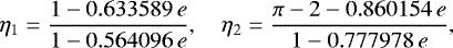
Odell & Gooding (1986) provide a list of 12 different choices of the first guess (called starter therein), many of them implying the computation of transcendental functions. In particular, they find that the most convenient choice out of such list is that called S12, defined as follows,
![Mathematical equation: \begin{equation*} E^{\text{OG}}_0 = \begin{cases} (1-e) M + e \sqrt[3]{6 M}, & \text{for}\; 0\le M<\frac{1}{6}\;\text{rad},\cr (1-e) M + e\left[\pi -\frac{a(\pi-M)}{c+M}\right], &\text{for}\; \frac{1}{6}\;\text{rad}< M<\pi,\cr \end{cases}\end{equation*}](/articles/aa/full_html/2022/02/aa41423-21/aa41423-21-eq23.png) (13)
(13)
where
 (14)
(14)
As shown in Sect. 3.1, this seed still implies a significantly larger average number of iterations (outside the critical region) thanthe rational seed that will be designed below, besides requiring a control statement and one cubic root evaluation.
More recently, efficient starters for the elliptic KE have been proposed in Calvo et al. (2013); Elipe et al. (2017), resulting in particular in the “optimal” seed
 (15)
(15)
where
 (16)
(16)
 (17)
(17)
and
 (18)
(18)
As shown in Sect. 3.1, this starter performs significantly better than the OG seed, thus it can be considered a good reference forcomparisons. Moreover, it can also be used in the ENRKE routine as an alternative to our rational seed, since they have similar performances.
The default first guess in the ENRKE routine is based on obtaining a small average number of iterations and on simplicity requirements, according to the following criteria:
- 1.
Due to the conditional switch to the bisection algorithm, the routine does not use the CNR or OG131 iterations in the critical region, where the term 1∕f′ entering Eqs. (4) and (6) is very large. Therefore, no particular care is needed for such problematic values.
- 2.
The seed satisfies Eq. (10) for every value of M ∈ [0, π], and the solution will be extended also outside such interval using Eq. (2).
- 3.
The difference E0 − M is a simple ratio of two polynomials, in such a way that it does not imply any preprocessing or evaluations of transcendental functions.
- 4.
The difference E0 − M reaches the maximum value, be, in the right point, which is
 . Although the exact maximum value would be e, with b = 1, our numerical computations have shown that better results are obtained by taking b slightly smaller than 1, namely b = 0.999999.
 - 5.
The difference E0 − M has the correct value E0 − M = 0 for M = 0 and M = π.
A simple rational seed satisfying these criteria is,
 (19)
(19)
for M ∈ [0, π]. As shown in Sect. 3.1, this seed implies a significant reduction of the average number of iterations and of the execution time, as compared to the PC, Danby, and OG seeds, even if for some values of e and M it requires a larger number of iterations. Moreover, its average performance is equivalent to that of CAL optimal starter. In any case, the ENRKE routine given in Appendix A.1 can be considered as a template that can use any starter, including those designed in Calvo et al. (2013); Elipe et al. (2017); Raposo-Pulido & Pelaez (2017).
Finally, these ideas may also be applied to other modified versions of the NR method, such as those described inRaposo-Pulido & Pelaez (2017); Tommasini & Olivieri (2021), in which the expression for Δn in Eq. (4) includes higher-order derivatives of f and an additional square root.
2.1.3 The conditional switch to the bisection method
As shown in Tommasini & Olivieri (2021), any version of the NR method, in which derivatives of f are used for the iterations, is unavoidably affected by a limiting accuracy
![Mathematical equation: \begin{equation*} \mathcal{E}^{\text{NR}}_{\text{lim}} \simeq \max\left[ \frac{\epsilon}{\sqrt{2(1-e)}}, 2 \pi \epsilon\right],\end{equation*}](/articles/aa/full_html/2022/02/aa41423-21/aa41423-21-eq31.png) (20)
(20)
when M ∈ [0, 2π]. Moreover, the E dependence of the limiting error is (Tommasini & Olivieri 2021)
![Mathematical equation: \begin{equation*} \mathcal{E}^{\text{NR}}_{\text{lim,E}} \simeq \max\left[\frac{\epsilon E}{{1-e\cos E}}, \epsilon E\right].\end{equation*}](/articles/aa/full_html/2022/02/aa41423-21/aa41423-21-eq32.png) (21)
(21)
The second term to be compared in the max procedure is the unavoidable uncertainty on the variable E due to the machine precision, maxϵE = 2πϵ in the interval M ∈ [0, 2π] (Tommasini & Olivieri 2021). In double precision, this implies that no method can guarantee a better precision than ~ 1.4 × 10⁻¹⁵ rad in such intervals. Although for most values of e and M, this limit and Eqs. (20) and (21) are excellent approximations as they are written, our numerical scans show that there are values of e and M for which they hold within a factor bigger than 1, though still smaller than 2. This larger limiting accuracy may be attributed to the uncertainty of the error itself. Therefore the best global accuracy in double precision for M ∈ [0, 2π] will be defined more conservatively to be  rad. However, due to the first terms in Eqs. (20) and (21), there is a region corresponding to e > eswitch and 0 < E < Eswitch such that this accuracy cannot be attained using derivatives (Tommasini & Olivieri 2021).
In the case of the CNR method, Eq. (21), the values of eswitch and Eswitch corresponding to a given input tolerance  can be obtained by numerically solving the equations
 (22)
(22)
in which, tobe conservative, the additional factor 2 mentioned above has been introduced. For  rad, the numerical solution in double precision of the first equation is
  . Moreover, for e →1 the second equation gives Eswitch ≃ 0.30 rad, corresponding to Mswitch ≃ Eswitch − sin Eswitch ≃ 0.0043 rad (more conservatively the ENRKE routine takes Mswitch = 0.0045 rad in this case). For general values of the input tolerance
  , introducing the Taylor expansion of the cosine in Eq. (22), it can be seen that Eswitch and Mswitch should scale proportionally to
  and
and  , respectively. However, in order to also minimize the induced errors on the true anomaly (to be discussed in Sect. 4.1), we make a more conservative choice and always use the switch values defined for the best accuracy (in double precision),
 (23)
(23)
 (24)
(24)
With these definitions, our scans show that the CNR method, combined or not with the OG131 iterator, provides convergence to the solution of KE within tolerance  for all values of M ∈ [0, 2π] when e ≤ eswitch, and for values of M ∈ [Mswitch, 2π − Mswitch], for e > eswitch.
The remaining region of the (e, M) plane defines the ‘critical region’ in which Newton-Raphson method and its generalizations do not guarantee convergence within accuracy  , however precise a seed they use (Tommasini & Olivieri 2021). To circumvent this limitation, we designed a procedure for computing the solution E of KE for any (e, M) in the critical region using the bisection method. The advantage of switching to the bisection method is that its accuracy is only limited by the machine precision ϵE (Tommasini & Olivieri 2021), or more conservatively 2ϵE, so that it can attain any level
  rad for all values of e ≤ 1 − ϵ and M ∈ [0, 2π]. Once again,in our routines we make a more conservative choice and set the tolerance to
  for the bisection method in the critical region (for e > 0.99 and E < 0.3), since this choice also minimizes the errors on the true anomaly, as discussed in Sect. 4.1.
Even though it requires a relatively large number of iterations (on average 47, the maximum value being 70 when M → 0), each of them involving one sine evaluation, the bisection method is only used in a small M region, that is in a fraction 0.0045∕π of values of M in a homogeneous set for  . As shown in Sect. 3.1, due to the reduced M size of such critical region, the speed of the ENRKE routine is on average almost the same for e greater or smaller than eswitch.
More importantly, the implementation of the bisection method in the critical region facilitates covering the complete (e, M) domain at the best accuracy, thus avoiding the divergence of the error for e → 1 that affects the NR method and its generalizations (Tommasini & Olivieri 2021).
2.2 The ENP5KE routine
For any fixed value of e, the piecewise quintic polynomial interpolation S(M) of the solution of KE is obtained by evaluating a polynomial,
![Mathematical equation: \begin{equation*} S_{j}(M) = \sum_{q=0}^{5} c^{(q)}_{j} \left[D_{j} (M - M_{j}) \right]^q,\end{equation*}](/articles/aa/full_html/2022/02/aa41423-21/aa41423-21-eq48.png) (25)
(25)
where j identifies the interval for which Mj ≤ M|[0,π] < Mj+1, with M|[0,π] being the value lying in the interval [0, π] corresponding to M by taking into account Eqs. (2). The resulting piecewise polynomial interpolation S can be considered to be continuous for M = Mj within the errors, the discontinuity being guaranteed to be smaller than the accuracy.
The breakpoints Mj are computed from an optimized grid Ej in a preprocessing phase as shown in Sect. 2.2.1, along with their associated k-vector and the coefficients Dj and  , whose numerical values depend on the value of e. This task is executed only once. This preprocessing phase, described in Sect. 2.2.1, accepts as inputs the value of the eccentricity e and the maximum error,
![Mathematical equation: \begin{equation*} \mathcal{E}\equiv \max_{M\in [0,2\pi]}\vert S(M) - E(M)\vert, \end{equation*}](/articles/aa/full_html/2022/02/aa41423-21/aa41423-21-eq50.png) (26)
(26)
tolerated for the solution when M ∈ [0, 2π]. Notice that ENP5KE routine works for any values of M, even though the breakpoints Mj = Ej − e sin Ej, and the optimized grid points Ej, belong to the interval [0, π]. For convenience of use, however, the values of the absolute error  are given for one full turn, namely M ∈ [0, 2π].
From a numerical point of view,  can be computed by comparing the results for S(M) over M ∈ [0, 2π] with those obtained with a grid using a reduced spacing. The output of this preprocessing phase are the arrays of the breakpoints Mj, the coefficients
  and the components kj of the k-vector. In the implementation of the routine, these parameters can be saved to a binary file, or retained in RAM once calculated for use in the subsequent call to the evaluate function. The generation phase, in which the solution of KE is obtained for any input value M by using Eq. (25), is described in Sect. 2.2.2. It requires: (i) the identification of the interval j between consecutive breakpoints Mj such that Mj ≤ M|[0,π] < Mj+1, with M|[0,π] being the value lying in the interval [0, π] corresponding to M by taking into account Eqs. (2); and (ii) the evaluation of the sum of products entering Eq. (25), involving the value of M and the precomputed parameters. The values S(M), interpolating E(M), are the final output of the procedure. In the critical region, defined as for the ENRKE routine, the evaluation step (ii) is modified by combining the use of the breakpoints for close bracketing of the solution, followed by continuous root search with the bisection method.
As shown in Sect. 2.2.3, the accuracy of this scheme can attain the best allowed level for a given machine precision. In particular, in double precision and for M ∈ [0, 2π] and e ≤ 1 − ϵ, the scheme converges with an error that can be controlled at the level  rad everywhere.
The speed performance of the ENP5KE will be discussed in Sect. 3.2. Since no transcendental functions are computed in the generation phase except in the critical region, this method outperforms the alternative algorithms, including the ENRKE routine, when the solution of KE is requested for a large number of values of M. Moreover, it is still very fast even for critical values of e and maximum accuracy.
2.2.1 Preprocessing and setup
The coefficients, breakpoints and associated k-vector are computed in the routine ENP5KE_coef. They are calculated on an optimized grid that is generated previously with a multistep routine, called ENP5KE_mstep, which provides a set of values Ej ∈ [0, π], for j = 0, …, n, corresponding to the values Mj = Ej − e sin Ej for the breakpoints. The expressions for the coefficients of Eq. (25) are given by
![Mathematical equation: \begin{equation*} c^{(q)}_{j} = \frac{1}{q! \, D_{j}^{q}} \left[ \frac{\partial^{q} E}{\partial M^q}(e, M_{j})\right],\end{equation*}](/articles/aa/full_html/2022/02/aa41423-21/aa41423-21-eq55.png) (27)
(27)
for j = 0, …, n − 1, where for computational convenience the first derivative
 (28)
(28)
has been introduced to the power of q in the denominator, compensating its presence in the numerator of Eq. (25).
The higher order derivatives of Eq. (28) are computed as in Stumpff (1968); Colwell (1993); Tommasini (2021). The resulting expressions for the coefficients are given in the listing of routine ENP5KE_coef in Appendix A.2, in terms of the quantities sj ≡ sin Ej, cj ≡ cos Ej, dj ≡ Dj, and dej ≡ Dj sin Ej. Their computation only implies the division of Eq. (28), so that zero divisions are avoided if 1 − e cos Ej ≥ ϵ, where ϵ is the machine epsilon, ϵ ≃ 2.22 × 10⁻¹⁶ in double precision arithmetic. This condition is satisfied for all Ej if
 (29)
(29)
The steps hj = Ej+1 − Ej in routine ENP5KE_mstep are chosen in such a way that higher order terms in Eq. (25) are smaller than lower order ones. Using the notation of routine ENP5KE_coef, the absolute values of the quantities sj and cj are always bounded below 1. Moreover, dj and dej are also of the order of 1 for most values of e, Ej, however they can be very large when 1 − e cos Ej ≪ 1, a regime corresponding to 1 − e ≪ 1 and  . In this regime,
  , so that dj
  and dej
  , and it can be seen that
  for q ≥ 2. Because |Dj (M − Mj)|≃|E − Ej|≾ hj, the contributions of orders q and q + 1 can be compared as follows,
![Mathematical equation: \[ \left\vert \frac{c^{(q+1)}_{j} \left[D_{j} (M - M_{j}) \right]^{q+1}}{c^{(q)}_{j} \left[D_{j} (M - M_{j}) \right]^q } \right\vert \lessapprox \begin{cases} \frac{h_j}{\sqrt{1-e}}, \; \text{for}\; 1-e\cos E_j\ll 1, \\ h_j, \; \text{for}\; 1-e\cos E_j\approx 1. \\ \end{cases} \]](/articles/aa/full_html/2022/02/aa41423-21/aa41423-21-eq63.png)
Therefore a choice of hj that would ensure that the coefficients get smaller for higher p for all values of e and Ej would be
 (30)
(30)
with a constant h(0) ≪ 1.
Since terms up to fifth-order are included in Eq. (25), the error  should scale as the sixth power of hj. Again, our numerical simulations show that this scaling law is an excellent approximation, thus the value of h(0) corresponding to an error level
  can be chosen to be
 . For any value of e, the coefficient γ(e) must ensure that the absolute error is smaller than the accuracy
  for every M ∈ [0, 2π]. We performed scans for many different values of e and found that the data for the largest γ(e) that is compatible with the error could be fitted from below with a quadratic dependence of e, namely
  . This result can be used to define a conservative choice for h(0), always producing errors below the level
  ,
,
![Mathematical equation: \begin{equation*} h^{(0)} = \left[0.86 + 1.1\, (1-e)+ 1.5\, (1-e)^2\right] \mathcal{E}^{1/6},\end{equation*}](/articles/aa/full_html/2022/02/aa41423-21/aa41423-21-eq71.png) (31)
(31)
with both h(0) and  being given in rad. For
  , this scaling law only breaks down in the critical region, that is when both e > eswitch and M < Mswitch (or 2π − Mswitch < M ≤ 2π), with eswitch and Mswitch defined in Eqs. (23) and (24) as for the ENRKE routine. In this region, a lower limit on the accuracy of the piecewise quintic polynomial is found at a level similar to that obtained for the Newton-Raphson method and its generalizations in Sect. 2.1.3.
As we shall discuss in Sects. 2.2.2 and 2.2.3, in such critical region the generation phase of the ENP5KE includes a switch to the use of the breakpoints of the piecewise polynomial for close bracketing, followed by bisection root searching. Due to this strategy, the accuracy of the ENP5KE routine in double precision can be set to the level  rad for every M ∈ [0, 2π] and e ≤ 1 − ϵ.
Equation (30) can be used to obtain an estimate of the number n of grid intervals for a given value of e. Since  , Eq. (30) implies,
![Mathematical equation: \begin{equation*} n \simeq \int_0^{\pi} \frac{\mathrm{d} E}{h^{(0)}\, \sqrt{1-e \cos E}} \lesssim \frac{1}{h^{(0)}} \left[\pi - \frac{\log(1-e)}{\sqrt{2}}\right] \equiv n_{\text{app}}.\end{equation*}](/articles/aa/full_html/2022/02/aa41423-21/aa41423-21-eq76.png) (32)
(32)
The value of napp is a good upper estimate of n, and is used in the wrapper class ENP5KE, listed in Appendix A.2, for allocating the memory of the array Ej before the call to the multistep routine ENP5KE_mstep. This function returns the array Ej and the correct value of n, which is then used for the memory allocations of the arrays Mj, kj, and  .
.
In addition to computing the breakpoints and the coefficients, the routine ENP5KE_coef also returns the k-vector that describes the nonlinearity of the set of the breakpoints, which will be used in the generation phase for the identification of the interval j. In fact, the k-vector provides the most efficient tool for close bracketing in large data sets (Mortari & Neta 2000; Mortari & Rogers 2013). The computation of kj in the routine ENP5KE_coef follows closely that given in Tommasini & Olivieri (2020b), with two simplifications. First, it avoids the introduction of two auxiliary parameters, called qkv and mkv in Tommasini & Olivieri (2020b), which may be useful for more general applications of k-vector search (Mortari & Neta 2000; Mortari & Rogers 2013), but which turn out to be irrelevant for the ENP5KE method. Second, it also avoids the use of the auxiliary array deltakv of Tommasini & Olivieri (2020b).
In Appendix A.2, an option is included that directs the code, specifically the code block within loop over j, to be run in parallel threads of execution on different CPU cores. This may reduce the CPU preprocessing time on most modern hardware without incurring perceivable overhead.
Finally, in the code implementation listed in Appendix A.2, the __init__ constructor function in the wrapper class ENP5KE also provides the option of saving the arrays of the breakpoints, the coefficients, and the k-vector to a binary file. In this case, because of the I/O bus bottleneck, the total execution time for the preprocessing phase is larger than retaining the parameters in RAM, possibly by an order of magnitude, depending on the hardware.
2.2.2 Generation of the solution
The generation phase of the algorithm returns the values S(Ma) that interpolate the solution of KE, E(Ma), for each input value Ma of the mean anomaly, for a = 0, …, N − 1 (Ma and S(Ma) can be considered as arrays with N elements). This phase of the algorithm is implemented in the function call interface (given by the override object, __call__) in the wrapper class ENP5KE. For each value of Ma, this process requires two steps:
- 1.
The identification of the jth interval. This task is performed in the find_interval function by using the k-vector for close bracketing of j, followed by (discrete) bisection. This routine is similar to that used in the cubic spline algorithm for function inversion of Tommasini & Olivieri (2020b), with a few important differences. First, it does not include the _us (use sorted) variant of Tommasini & Olivieri (2020b), which allowed for a significant speed improvement when the input array was sorted, but required using the result of the previous search. By making all individual searches independent, the new find_interval routine can be run in parallel from ENP5KE_evaluate, with a speed gain that can be larger than the loss due to renouncing the _us variant, and with increasing advantage the larger is the number of cores of the CPU. Second, the routine has been simplified, and the use of the mkv and qkv parameters of Tommasini & Olivieri (2020b) has been avoided. Third, the addition of the control sequence if x[left + 1] > xval: return left, followed by the line left = left + 1, just before the bisection run, keeps the average number of bisection iterations below ~ 0.5 for all values of e, for large N and uniform random arrays Ma (see Sect. 3.2). Even if these discrete bisection iterations are very fast, since they only involve one control sequence with an elementary operation using values from a precomputed array (no transcendental function is evaluated), reducing their average number well below one still results in a nonnegligible speed improvement.
- 2.
The evaluation of the sum of products of Eq. (25), involving the value of M and the breakpoints and coefficients given in the precomputed arrays, is performed by the Cython routine ENP5KE_evaluate. In the critical region e > eswitch, and M < Mswitch (or 2π − Mswitch < M ≤ 2π), this evaluation step is modified by combining the use of the breakpoints for close bracketing of the solution, followed by continuous root search with bisection. The latter, involving a sine computation for each iteration, is the only procedure implying the computation of transcendental functions in the generation phase of the ENP5KE, and it is only required in a very small region of the parameter space. In all cases, the option of running the for loop over a = 1, …, N in parallel can provide speed improvements which become more relevant for larger values of N and increased number of CPU cores.
2.2.3 The conditional switch to the bisection method
We verified empirically that Eqs. (30) and (31) ensure convergence of the piecewise quintic polynomial up to a limiting accuracy of the order ![Mathematical equation: $\max\left[ \frac{2\epsilon}{\sqrt{2(1-e)}}, 4 \pi \epsilon\right] $](/articles/aa/full_html/2022/02/aa41423-21/aa41423-21-eq78.png) , when M ∈ [0, 2π]. This is the same limiting accuracy that applies to all implementations of Newton-Raphson (NR) algorithm and its generalizations in such M interval, as discussed in Sect. 2.1.3. The reason for reaching a similar limiting precision lies in the use of the derivative terms 1∕(1 − e cos E), which enter into the higher order coefficients in the case of the ENP5KE.
, when M ∈ [0, 2π]. This is the same limiting accuracy that applies to all implementations of Newton-Raphson (NR) algorithm and its generalizations in such M interval, as discussed in Sect. 2.1.3. The reason for reaching a similar limiting precision lies in the use of the derivative terms 1∕(1 − e cos E), which enter into the higher order coefficients in the case of the ENP5KE.
As in Sect. 2.1.3, the best testable accuracy in double precision for M ∈ [0, 2π] will be defined to be  rad, as for the ENRKE routine. Again, there is a critical region corresponding to e > eswitch and 0 ≤ |M − Mp| < Mswitch (with Mp = 0 or 2π) such that this accuracy cannot be attained using derivatives, with the values of eswitch and Mswitch given in Eqs. (23) and (24). Although these estimates for the switch values have been obtained using the expression of the errors for NR method as given in Sect. 2.1.3, our numerical computations show that they apply also to our piecewise polynomial expansion. Of course, this is due to the fact that both methods use the inverse derivative
  . As discussed in Tommasini & Olivieri (2021), a similar limiting accuracy also affects algorithms using divisions involving small differences, like Inverse Quadratic Interpolation or the secant method (Brent 1973).
To circumvent such a constraint, for any e, M in the critical region the ENP5KE computes the solution E of KE using the precomputed grid interval Ej < E < Ej+1 for close bracketing and the bisection root search method for the final computation. (This continuous bisection search should not be confused with the discrete bisection that is used to identify the interval j after the k-vector bracketing, and that only implies a very small number of steps, which only involve precomputed values without any transcendental function evaluations.) As a result, the accuracy of the ENP5KE can attain the optimal level  rad for all values of e ≤ 1 − ϵ and M ∈ [0, 2π], including inthe critical region, where it is set to the more conservative best choice
  as in Sect. 2.1.3 in order to also minimize the errors on the true anomaly.
This  is set as the default value for the tolerance in the ENP5KE. The price to pay is iterations with function evaluations, namely one sine for each step when the continuous bisection method is used. This makes the speed of the ENP5KE slower in the critical region than for any other values of e, M, although thanks to the reduced size of such region, the close bracketing, and the optimal Cython implementation, the average speed records remain impressive everywhere, as shown in Sect. 3.2.
The reason for such an excellent performance can be understood by computing the number of bisection iterations  needed to obtain the solution E with tolerance
  in a given interval j of the singular region. When M belongs to the jth grid interval of step hj, the condition
  implies
![Mathematical equation: \begin{eqnarray*} n^{\text{bis}}_j &\simeq& \frac{1}{\log_{10} 2}\log_{10}\frac{h_j }{(10^{-7} + \frac{E}{0.3})\,\mathcal{E}}\nonumber\\ & \simeq& 3.32 \log_{10} \left[0.86\, \left(10^{-7} + \frac{E_j}{0.3}\right)^{-1}\,\mathcal{E}^{-5/6}\, \sqrt{1-e\cos E_j} \right], \end{eqnarray*}](/articles/aa/full_html/2022/02/aa41423-21/aa41423-21-eq87.png) (33)
(33)
where Eqs. (30) and (31) have been used (for e close to 1). Taking also  , we can estimate the maximum number of bisection iterations for e > 0.99, and obtain
  . This maximum is only reachedvery close to M = 0, the most common values, obtained for 10−7 rad ≪ E ≤ 0.3 rad, being
  . Each bisection iteration implies one computation of f(E), that is one sine evaluation. Such iterations are only required for e > eswitch = 0.99, and for such values of e they have to be performed only for 0 < M < 0.0045 or M < 2π − 0.0045. Usually, KE has to be solved on an uniform time array. In this case, the bisection root search method only has to be used in a fraction 0.0045∕π = 1.4 × 10⁻³ of the time (that is M) points. Since KE is solved noniteratively using only the precomputed coefficients and without any transcendental function evaluation for the rest of values of M, the average number of transcendental functions evaluations per solution is 38 × 1.4 × 10−3 ≃ 0.054. Therefore, even for e > eswitch = 0.99, when it is complemented with bisection root search for 0 ≤ M < 0.0045 or 2π − 0.0045 < M ≤ 2π, the ENP5KE routine remains very fast, requiring only ~0.054 transcendental function evaluations per solution on average.
Even more importantly, as for the ENRKE, the implementation of bisection in the critical region facilitates covering the complete (e, M) domain at the best accuracy.
Figures 1 and 2 display the M distribution of the errors for four different values of e and three choices of the input accuracy,  rad,
rad,  rad, and
  10−15 rad. It can be seen that the error is controlled below the chosen level even when e differs from 1 only by the machine epsilon. This conclusion has also been confirmed with scans using a logarithmic scale for M to better sample the critical region. We have checked that similar results can be obtained for every value of e ≤ 1 − ϵ.
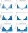 |
Fig. 1 M dependence of the errors of the ENP5KE algorithm for solving KE in double precision for e = 0.8 (left) and e = 0.99 (right), when the input accuracy (tol) is set to the level 3 × 10⁻⁹ rad (top), 3 × 10⁻¹² rad (center), and 3 × 10⁻¹⁵ (bottom). For these values of e, the solutionis obtained using the piecewise quintic polynomial only, without the need for continuous bisection root search. |
3 Results
3.1 Performance of the ENRKE routine
In order to have a reference for comparisons, Table 1 shows the performance of the CNR method with the classical stopping condition for different values of the eccentricity e, when the tolerance is set to the value  rad for M ∈ [0, 2π]. Since the implementations described in this table do not use the conditional switch to the bisection method in the critical region, only the values of e ≤ 0.99 can be given for this accuracy level. The presented results correspond to four different choices of the starter. In all cases, the average CPU time per solution tgen ∕N (in nanoseconds), calculated by dividing by N the time for computing N = 108 solutions of KE (corresponding to N equally spaced values of M), was obtained with similarly optimized Cython routines executed in parallel on a laptop computer with modest hardware (a 64 bit Intel i7-8565U CPU 1.8 GHz × 4 cores, with 16 GB RAM, and with Linux Mint operating system with 5.4.0–65 kernel). Such average CPU times have been obtained by averaging tgen ∕N over 10 runs of each case (each with aloop over N = 108 values of M), and an error of ~1 has to be understood affecting the last digit, in this case corresponding to an error ~ 1 ns/sol. In contrast,the values of the average and maximum number of CNR iterations,
  and
and  , do not depend on the hardware and are determined with greater precision.
As can be seen, the rational seed of Eq. (19) allows for a significant reduction of the average number of CNR iterations,  , and of the execution time, as compared to the PC and OG seeds, even though for some values of e the maximum number of iterations
  may be higher than with the OG starter. Its performance in terms of the average number of iterations is slightly worse or better than that of CAL optimal starter for e < 0.5 of e ≥ 0.5, respectively, the resulting difference in CPU execution time being not significant within the error affecting tgen∕N.
Table 2 presents the performance of the complete ENRKE routine using our rational seed, also including the switch to bisection in the critical region, one run of the OG131 iterator, and the efficient iteration stopping condition of Eq. (9).
As can be seen, the switch to the bisection method in the critical M region for e > 0.99 implies a small CPU time increment of ~1 nanosecond/solution, on average, as compared with the performance for e ≤ 0.99. However, such a switch ensures a dramatic enhancement of the precision, as discussed in Sect. 2.1.3, facilitating the computation of the solution of KE also for values of e > 0.99 at the best attainable accuracy. Remarkably, even with such modest hardware, the highly optimized, parallel ENRKE routine, solves KE with the best allowed accuracy  rad in just ~ 20 nanoseconds per solution on average (in the high N regime), even for e equal to 1 within machine epsilon. By comparing Tables 1 and 2, it can also be seen that the use of one OG131 iteration and of the efficient stopping condition of Eq. (9) imply a reduction of more than ~ 1.5 average iterations per solution, and a speed increase of a factor ~2, with respectto the performance of the CNR method with the classical stopping condition using the same seed or CAL starter. The improvement is even higher when the comparison is made with the CNR method with the PC or OG seeds. Remarkably, the ENRKE routine requires 2.19 × 2 + 0.068 = 4.45 transcendental function evaluations on average, even for e → 1, to attain thebest accuracy 3 × 10⁻¹⁵ rad.
Finally, we checked that the use of parallel computing (with prange in the ENRKE_evaluate routine) implies a factor ~ 3 speed improvement, as compared with the same loop being executed sequentially (with range). This speed improvement, which is understood in both Tables 1 and 2, is expected to be even larger for hardware with more cores.
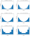 |
Fig. 2 M dependence of the errors of the ENP5KE algorithm for solving KE in double precision for e = 0.999 (left) and e = 1 − ϵ (right), when the input accuracy (tol) is set to the level 3 × 10⁻⁹ rad (top), 3 × 10⁻¹² rad (center),and 3 × 10⁻¹⁵ (bottom). For these values of e, the solution is obtained using the piecewise quintic polynomial for 0.0045 rad ≤ M ≤ 2π − 0.0045 rad, and with breakpoint bracketing followed by continuous bisection root search in the intervals M < 0.0045 rad and M > 2π − 0.0045 rad. |
Performance of the CNR solution of KE with different seeds.
Performance of the ENRKE routine.
3.2 Performance of the ENP5KE routine
Table 3 shows the performance of the ENP5KE routine for different values of the eccentricity e, when the accuracy is set to the value  . The values of n required for higher values of the error level
  can be obtained by scaling those listed in Table 3 with the factor
  . The last three columns indicate the time performances obtained using the same modest hardware as in Sect. 3.1 (a 64 bit Intel i7-8565U CPU 1.8 GHz × 4 cores, with 16GB RAM, and with Linux Mint operating system with 5.4.0–65 kernel). It can be seen that even at the best accuracy, the CPU time tinit needed to compute the coefficients, breakpoints, and k-vector, is at the level of ~ 10−4 s or in any case below a millisecond, thus being more than an order a magnitude smaller than the setup time required with the cubic spline inversion algorithm of Tommasini & Olivieri (2020a,b). Of course, another advantage of the ENP5KE, as compared to the method of Tommasini & Olivieri (2020a,b), is that it can reach the best accuracy
  even in the critical region.
The average CPU time per solution tgen∕N has been obtained by dividing by N the time for computing N = 108 solutions of KE (corresponding to N equally spaced values of M), running the ENP5KE routine in parallel. Even with the modest hardware used in our simulations, each solution requires, on average, at most 2.8 nanoseconds, for e ≤ eswitch = 0.99, and 4.0 nanoseconds for e > eswitch = 0.99. A significant part of the difference between the values of tgen∕N for e lower or higher than eswitch is due to the control sentence if (sw == 1 and Mjr < Msw): in the function ENP5KE_evaluate. In fact, when this check is also (unnecessarily) included in the routine for e < eswitch, the values oftgen∕N also grow by~0.5 ns. Remarkably, the ENP5KE routine is so fast that even a single control sequence that does not involve any transcendental function evaluation can produce a small but appreciable increase in the execution time. In order to avoid such an increase, the users can comment this control environment in ENP5KE_evaluate if they do not need to use the routine for e > eswitch.
Comparing with the results of Table 2, it can be seen that in the large N regime the ENP5KE is faster than the similarly optimized ENRKE routine by a factor 5–6, in speed. The difference is larger when the comparison is made with the results given in Table 1 for the CNR method, even when it uses the optimal CAL starter.
As for the ENRKE routine, we also checked that the use of parallel computing (with prange in ENP5KE_evaluate) implies a factor ~ 3 speed improvement for the ENP5KE, as compared with the same loop being executed sequentially (with range). This speed improvement, which is understood in Table 3, is expected to be even larger for hardware with more cores.
Performance of the ENP5KE routine.
4 Discussion
The efficiency of any KE solver is measured by its accuracy and by its speed.
The accuracy is constrained by the two limits due to the roundoff errors demonstrated in Tommasini & Olivieri (2021), which should be multiplied by an additional factor ~2 to be strictly valid for every e and M, as discussed in Sect. 2.1.3:
The universal limit on the relative error affecting the eccentric anomaly E is the machine epsilon, ϵ. For nturn turns, in which M and E vary by 2 π nturn, this implies a limiting absolute error ≃ 2 π ϵ nturn. In practice, as discussed in Sect. 2.1.3, we found that an additional factor ~ 2 in one turn was recommended, and defined the best testable error in double precision to be
 rad for the interval M, E ∈ [0, 2π]. We also verified that, once the tolerance of the ENRKE or ENP5KE routines is set to a value
  over the interval M, E ∈ [0, 2π], the maximum absolute error affecting the solution E for M, E > 2π grows linearly as
  , as to be expected from the universal limit on the relative error mentioned above.
-
The second limit, also demonstrated in Tommasini & Olivieri (2021), constrains the accuracy of all the KE solvers that use the derivative term
 or divisions by differences between close values of E. After multiplying by the additional factor ~2 discussed in Sect. 2.1.3, such a limit would imply that the minimum allowed error would be at least
  , which is larger than
  for e > 0.99 (in double precision). Fortunately, this limit can be circumvented with the conditional switch to the bisection method that we introduced in our ENRKE and ENP5KE routine, and which can also be implemented in other KE solvers to enhance their accuracy for high eccentricity orbits, as we shall show in Sect. 4.3. Besides being necessary for improving the accuracy, this conditional switch can also have beneficial side effects on the speed performance, since it removes the need to deal with diverging derivative terms. As seen for the ENRKE routine in Sect. 2, this switch also allowed for implementing our efficient iteration stopping condition. Moreover, as we shall discuss in Sect. 4.1 below, the use of the bisection method with tolerance set to
  in the critical region facilitates the control of the precision for the resulting true anomaly for all values of e and M. Another example in which this conditional switch is also of great help for the speed performance will be given in Sect. 4.3 below.
Alternatively, Farnocchia et al. (2013) proposed a method for obtaining the time evolution of elliptic orbits for critical values of e and M by avoiding the direct solution of KE, and thus the diverging derivative term  . Users familiar with their method might use our routines for all other values of e and M, and switch to their algorithm, as an alternative equivalent to using bisection, in the critical region (e > 0.99 and M within 0.0045 rad from periapsis). In any case, this change is not expected to significantly affect the average execution time over an equally spaced array of values of M ∈ [0, 2π], as compared to that using the switch to the bisection method. In fact, the speed of the ENRKE and ENP5KE was already quite similar for e = 0.99 (value that did not include the critical region) or for e = 0.999 (for which the critical M region was included), the difference in execution time being just ~1 ns/solution, on average, on the modest hardware used for the simulations of Tables 2 and 3.
The speed of a KE solver can be optimized with the following strategies:
-
Reducing the number of operations, and especially the number of transcendental function evaluations. A simple numerical example can be used to illustrates the rationale behind this point. We compared the CPU time for computing (i) sin (x), (ii)
![Mathematical equation: $\sqrt[3]{x}$](/articles/aa/full_html/2022/02/aa41423-21/aa41423-21-eq112.png) (the cubic root), (iii) the product xx. The computation has been performed in double precision using the same hardware as in Sect. 3 on 108 homogeneous random points with sequential computing using a Cython routine compiled in C, so that the execution times are similar to those that can be obtained in pure C. The results for the CPU execution time in the three cases mentioned above are (i) (the sine) tCPU = 0.95 s, (ii) (the cubic root) tCPU = 1.8 s, (iii) (the product) tCPU = 0.13 s (of course, the time for generating the random array is not included in these execution times). Thus the computation of the cubic root using the standard C math function from the Cephes (Moshier 2000) mathematical library, namely cbrt.c, is more time consuming (by a factor ~2) than that of one transcendental function call because it requires two floating-point manipulations (with frexpl and ldexpl) equivalent to one logarithm and one exponential calls. This also implies the known recommendation of avoiding the use of powers when possible, and for example, compute the product xx rather than the power x2. In summary, an efficient routine tries to reduce the number of operations, prioritizing the reduction of the calls to transcendental functions.
(the cubic root), (iii) the product xx. The computation has been performed in double precision using the same hardware as in Sect. 3 on 108 homogeneous random points with sequential computing using a Cython routine compiled in C, so that the execution times are similar to those that can be obtained in pure C. The results for the CPU execution time in the three cases mentioned above are (i) (the sine) tCPU = 0.95 s, (ii) (the cubic root) tCPU = 1.8 s, (iii) (the product) tCPU = 0.13 s (of course, the time for generating the random array is not included in these execution times). Thus the computation of the cubic root using the standard C math function from the Cephes (Moshier 2000) mathematical library, namely cbrt.c, is more time consuming (by a factor ~2) than that of one transcendental function call because it requires two floating-point manipulations (with frexpl and ldexpl) equivalent to one logarithm and one exponential calls. This also implies the known recommendation of avoiding the use of powers when possible, and for example, compute the product xx rather than the power x2. In summary, an efficient routine tries to reduce the number of operations, prioritizing the reduction of the calls to transcendental functions.The ENRKE iterative routine pursues this strategy by enhancing Newton-Rapshon method with an efficient stater, a run of Odell-Gooding fourth-order iterator, and an improved stopping conditions that allows for avoiding almost ~ 1 (on average) Δ computations and save one sine and one cosine evaluations. Such stopping condition can also be applied to enhance other methods. The reliability of the ENRKE routine and of its stopping condition will be further discussed in Sect. 4.2 below.
The ENP5KE routine pursues a different variant of this strategy by concentrating all the transcendental function evaluations in a setup or preprocessing phase (besides a minimum amount that is required in the critical region). As such, this routine is convenient when the solution of KE is requested over a large number of values of M, so that the time for the preprocessing can be neglected.
Implement the algorithm as a specifically tailored routine aimed at achieving high-performance by compiling with optimization switches directed toward the specific CPU platform to be used and by multithreaded parallel programming that targets the specific memory and multicore hardware. Both the ENRKE and ENP5KE routines use this strategy, and they can be used as templates for the high-performance implementation of other algorithms, as shown in Sect. 4.3.
4.1 Errors on the true anomaly
In this section, we derive the errors Δθ on the true anomaly,
![Mathematical equation: \begin{equation*} \theta = 2\arctan \left[\sqrt{\frac{1+e}{1-e}}\tan\frac{E}{2}\right],\end{equation*}](/articles/aa/full_html/2022/02/aa41423-21/aa41423-21-eq113.png) (34)
(34)
induced by the uncertainty ΔE on the eccentric anomaly. When ΔE is small enough, Δθ can be computed with the usual rule for error propagation,
 (35)
(35)
For small values of e, the resulting error on the true anomaly is of the same order of the accuracy level  that has been set for E. In general, for any e and M outside the critical region, the largest value of Δθ is attained for e = 0.99 and M = E = 0, so that
 (36)
(36)
If  rad, this gives Δθ < 4.3 × 10⁻¹⁴ rad.
In the critical region, the choice made in Sects. 2.1.3 and 2.2.3,  , facilitates controlling the error below the same level,
  , for all values of e ≤ 1 − ϵ and M ∈ [0, 2π].
In summary, when the input tolerance  for E is set to the value 3 × 10⁻¹⁵ rad in our ENRKE, ENP5KE, or ENMAKE routines, the true anomaly given by Eq. (34) will be obtained with an accuracy of 4.3 × 10⁻¹⁴ rad for all values of e ≤ 1 − ϵ and M ∈ [0, 2π], the actual error being as low as ~3 × 10⁻¹⁵ rad for small e.
4.2 Reliability of the error analysis and of the enhanced iteration stopping condition for the ENRKE method
Here we discuss the validity of the approximation  that was used in Sects. 2.1.1 and 2.1.3.
From Eq. (3), we obtain,
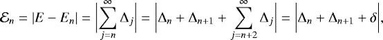 (37)
(37)
where we defined  . In particular, this also implies that
  .
.
These equations can be used to obtain the inequalities,
 (38)
(38)
and therefore
 (39)
(39)
Since our iteration stopping condition (9) is applied to the CNR method, the n dependence of the errors is given by Eq. (8). Because En and Ēn should converge to the exact solution E, we can approximate the coefficient of  in such an equation with its asymptotic value
  in Eq. (8). From a perturbative point of view, the effect of this approximation is expected to be of higher order in the errors. As a result, we can assume that
  . Substituting in the inequality (39), we obtain,
 (40)
(40)
Isolating |Δn| we finally obtain,
 (41)
(41)
Therefore ![Mathematical equation: $\Delta_n = \mathcal{E}_{n}[1+\mathcal{O}(\beta\, \mathcal{E}_n)]$](/articles/aa/full_html/2022/02/aa41423-21/aa41423-21-eq132.png) . As a consequence, since the uncertainty on the error is a higher order effect, the approximation
. As a consequence, since the uncertainty on the error is a higher order effect, the approximation  is expected to be valid when
  . Because the maximum value of β outside the critical region is ≃ 3.5, this condition is generally attained for
  rad. Even less stringent limits apply for small eccentricity, e ≪ 1, since in this case β ≪ 1 and the condition
  rad is satisfied even when
  is of order 1. We note that the conditional switch to the bisection method in the critical region is the key for the approximation
  to be valid, since it facilitates avoiding larger (and eventually diverging) values of β.
Moreover, our enhanced stopping condition, Eq. (9), can be rewritten as,
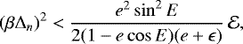 (42)
(42)
where, once again, we approximated En with its asymptotic value E. When e → 1, the identity sin2E = (1 − cos E)(1 + cos E) can be used to show that  rad ensures that β Δn ≲ 10−2. It can be seen that this condition on
  is also sufficient to have βΔn ≪ 1 for all values of e and E outside the critical region.
In summary, as a consequence of the conditional switch to the bisection method in the critical region, all the approximations underlying our enhanced stopping condition, Eq. (9), are expected to be valid provided that the accuracy is set to a level  rad.
rad.
4.3 Enhancing Markley’s KE solver
In this subsection, we discuss another example showing how an existing iterative KE solver can be enhanced using the conditional switch to the bisection method for improving the accuracy, together with parallel computing for optimizing the speed performance. The example chosen to illustrate this procedure is Markley’s KE solver (Markley 1995). The starting point is the following approximate analytical solution of KE,
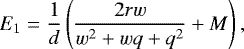 (43)
(43)
where
 (44)
(44)
and
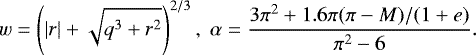 (45)
(45)
Up to this point, Markley’s solver implies one cubic root and one square root (which is equivalent to more than 2 transcendental function evaluations) for the generation of E1.
This approximate solution E1 is then used as the starter for a single run of a fifth-order iterator,
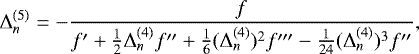 (46)
(46)
where
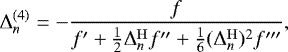 (47)
(47)
with  given in Eq. (5). The computation of
  involves twoadditional transcendental function evaluations. In the original solver (Markley 1995), further steps are performed to deal with the effect of the machine epsilon. However, since Markley’s method uses the derivative terms, it cannot overcome the accuracy limit discussed in Tommasini & Olivieri (2021) and in Sect. 2.1.3 without switching to a nonderivative method such as bisection in the critical region.
A high-performance Cython routine, called ENMAKE, enhancing Markley’s method with such a conditional switch to the bisection method in the critical region is provided in Appendix A.3. Our scans have shown that due to this switch this routine does not need any additional steps, besides the  iterator, to attain the best accuracy
  (in double precision) over the entire interval M ∈ [0, 2π]. This simplification is a side benefit of the conditional switch to the bisection method, since it allows for avoiding the additional steps introduced in Markley (1995).
As a consequence, the ENMAKE routine only requires the equivalent of 4–5 transcendental function evaluations so that its performance can be expected to be similar to that of the ENRKE routine. In fact, we found that the average CPU time required by the ENMAKE routine for computing 108 solutions of KE over an equally spaced array of values of M with accuracy  , under the same conditions and with the same hardware as in Table 2, is
  nanoseconds per solution. This average execution time, obtained with parallel computing, does not depend on e within the errors. By comparing with Table 2, it can be seen that the ENMAKE and the ENRKE routine are equivalent in terms of the average performance, besides attaining the best accuracy in both cases. These results are made possible by the conditional switch to the bisection method.
5 Conclusions
The numerical solution to the Kepler equation (KE) continues to be an active area of inquiry due to its essential role in many application areas of Astronomy and Astrophysics. Of particular interest for such solutions are both speed and accuracy. The contributions of this work are enumerated as follows.
- 1.
We described two methods, called ENRKE and ENP5KE, for solving the KE with both very high speed and the best attainable accuracy compatible with the given machine precision, circumventing the limit on the error demonstrated in Tommasini & Olivieri (2021) by avoiding the use of derivatives in the critical region, that is, e > 0.99 and M close to the periapsis within 0.0045 rad (in double precision).
- 2.
We provided high-performance Cython routines implementing these methods, with the option of utilizing parallel execution for multicore CPUs. Brief compilation instructions and basic usage have also been given in Appendix B.
- 3.
These routines solve KE for every value of the eccentricity e ∈ [0, 1 − ϵ], where ϵ is the machine epsilon (ϵ = 2.2 × 10⁻¹⁶ in double precision), and for every value of the mean anomaly M. In particular, for M ∈ [0, 2π], they can guarantee an accuracy at the level 3 × 10⁻¹⁵ rad (in double precision) even for e → 1 within the machine epsilon. This is the best testable global accuracy (within a factor ~1) that can be obtained with any method for solving KE in this M interval.
- 4.
When the input tolerance
 for the eccentric anomaly is set to the value 3 × 10⁻¹⁵
rad in our ENRKE, ENP5KE, or ENMAKE routines, the true anomaly θ
will be obtained with an accuracy of 4.3 × 10⁻¹⁴
rad for all values of e ≤ 1 − ϵ
and M ∈ [0, 2π], the actual error being as low as ~3 × 10⁻¹⁵
rad for small e.
for the eccentric anomaly is set to the value 3 × 10⁻¹⁵
rad in our ENRKE, ENP5KE, or ENMAKE routines, the true anomaly θ
will be obtained with an accuracy of 4.3 × 10⁻¹⁴
rad for all values of e ≤ 1 − ϵ
and M ∈ [0, 2π], the actual error being as low as ~3 × 10⁻¹⁵
rad for small e. - 5.
As mentioned in point (1), the existing claims that this accuracy level could also be reached with any method based on computing derivatives were recently disproved in Tommasini & Olivieri (2021). Therefore, the ENRKE and ENP5KE routines attain a record accuracy, which matches that of nonderivative algorithms such as the bisection root search method or that of strategies that avoid the direct resolution of KE (Farnocchia et al. 2013).
- 6.
The ENRKE routine enhances Newton-Raphson algorithm with (i) a conditional switch to the bisection algorithm in the critical region, (ii) a more efficient iteration stopping condition, (iii) a novel rational first guess, (iv) one run of Odell and Gooding’s fourth order iterator, and (v) the use of parallel execution.
- 7.
With these prescriptions, the ENRKE significantly outperforms other implementations of the Newton-Raphson method both in speed and in accuracy.
- 8.
Moreover, the ENRKE routine can also be seen as a template that can be easily modified to use any other starters and iterators. As such, it has been used to enhance Markley’s KE solver, resulting in a routine called ENMAKE, also given in the appendix. Due to the conditional switch to the bisection method in the critical region, this routine also attains the best accuracy in double precision, and it can be simplified in such a way that its average time performance is equivalent to that of the ENRKE routine.
- 9.
With the hardware used in our simulations (modest Intel i7/16 GB RAM), both the ENRKE and the ENMAKE have provided large numbers of solutions of KE, spending ~20 nanoseconds per solution on average, even at the limiting accuracy. These results have been obtained using parallel execution.
- 10.
The ENP5KE routine uses a class of infinite series solutions of KE to build a specific piecewise quintic polynomial for the numerical computation of the eccentric anomaly E, expressed in terms of power expansions of (M − Mj), where the breakpoints Mj are chosen according to a detailed optimization procedure. This method is also enhanced with a conditional switch to close bracketing and bisection in the critical region.
- 11.
Since it is specific to KE and it is of a higher order, the ENP5KE routine provides significant improvements with respect to the universal cubic spline for function inversion of Tommasini & Olivieri (2020a,b). In particular, it reduces the setup time and memory requirements by an order of magnitude. Even more importantly, because of the conditional switch to the bisection method, it can also attain the best allowed accuracy within the given machine precision.
- 12.
Since the generation phase of the ENP5KE routine does not involve any transcendental function evaluation, besides a minimum amount required in the critical region, it outperforms any other solver of KE, including the ENRKE, when the solution E(M) is required for a large number N of values of M.
- 13.
With the hardware used in our simulations (modest Intel i7/16 GB RAM), the CPU time for completing the setup phase of the ENP5KE routine has been of the order of ~10−4 s, and in general below the millisecond, even at the best attainable accuracy in double precision (that is 3 × 10⁻¹⁵ rad for M ∈ [0, 2π]).
- 14.
In the generation phase, the ENP5KE has provided large numbers of solutions of KE, spending at most 4 nanoseconds per solution on average (3 nanoseconds per solution for e ≤ 0.99) using parallel execution, even at the limiting accuracy.
- 15.
Since similar accuracy limits affect the solution of both the elliptic and the hyperbolic KE (Tommasini & Olivieri 2021), the ideas presented here may also be used to enhance methods that solve the latter, such as those described in Refs. (Gooding & Odell 1988; Raposo-Pulido & Pelaez 2018).
In summary, the ENRKE routine can be recommended as a general purpose solver for KE, and the ENP5KE can be the best choice when the solution is requested for a large number of values of M.
Acknowledgements
This work was supported by grants 67I2-INTERREG, from Axencia Galega de Innovación, Xunta de Galicia, andFIS2017-83762-P from Ministerio de Economia, Industria y Competitividad, Spain.
Appendix A Code listings
This appendix provides listings of the routines described in the text. They are given as Cython functions, which can also serve as pseudocodes due to the simplicity of the syntax. These routines can be included in a file, for example called Kepler_solver.pyx, which can be complied to C and imported from Python as discussed in Appendix B. The necessary libraries have to imported as shown in Sec. B.2, and three lines with the decorators of Sec. B.3 have to be added right before each function. The wrapper classes ENRKE and ENP5KE listed in Secs. A.1 and A.2 can then be imported in a Python file with the instruction
from Kepler_solver import ENRKE, ENP5KE
Two options are commented with a # in some routines:
-
The for loops in the coef and evaluate routines are executed in parallel when they are defined using prange. If the number of iteration is small, the option of using sequential computing, replacing prange with range, may be faster, depending on the number of cores and specific CPU architecture and latency. With the hardware used in our simulations (modest Intel i7/16GB RAM), range usually provided a better performance than prange in the routine ENP5KE_coef, in which the for loop runs at most over a few thousands of steps for every e and accuracy level.
In the evaluate routines, when the solution is requested also for values of M > 2π (as when more than one turn is considered), the line
Mjr = Mj%6.2831853071795864779
should be used to replace the line Mjr = Mj.
Secs. A.1, A.2, and A.3 present the listings of the routines entering the ENRKE, ENP5KE, and ENMAKE algorithms, respectively.
A.1 Routines for the ENRKE method
A first call to the ENRKE class from a Python code performs the initialization. The instruction for this step is:
S = ENRKE(ec, tol)
where the input parameters correspond to the eccentricity ec and the accuracy tol (if the latter is not specified, the default value 3 × 10⁻¹⁵ rad is assumed). Once S has been initialized as shown above, it can be called repeatedly with the instruction
S(M)
where M is a set (array) of N values of the mean anomaly for which the solution E of KE is requested. The values of the array S(M) will then be the ENRKE interpolations of the solution in the points M.
A.1.1 Function ENRKE_evaluate
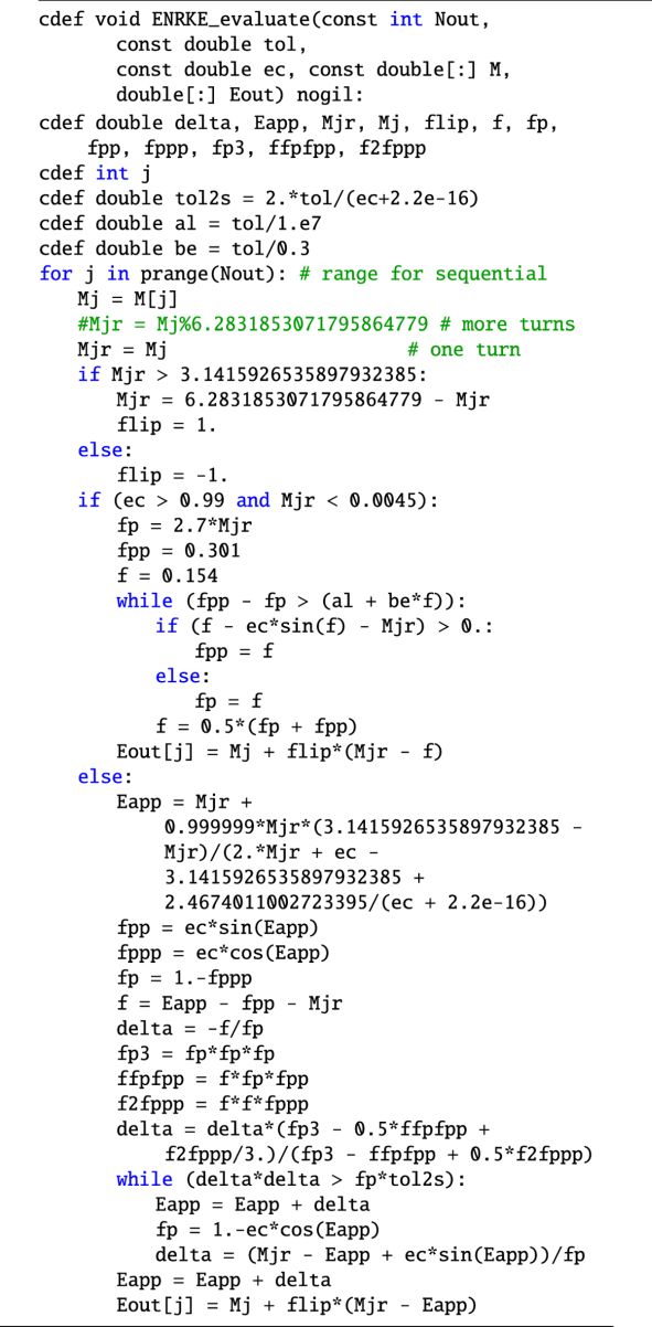
The lower bound E > 2.7M for e > 0.99 and M < 0.0045 originates from the limit obtained in Serafin (1986).
A.1.2 Wrapper class ENRKE
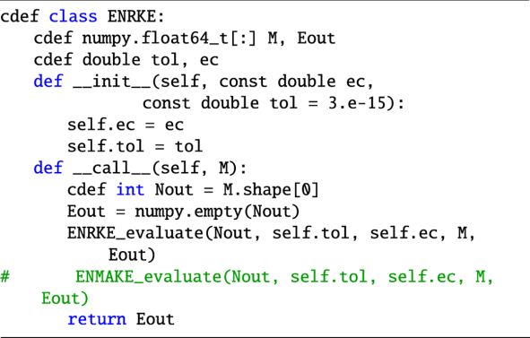
This wrapper class can also be used to call the ENMAKE routine, described in Appendix A.3, by commenting the line calling ENRKE_evaluate and uncommenting the call to ENMAKE_evaluate.
A.2 Routines for the ENP5KE method
A first call to the ENP5KE class from a Python code performs the initialization, computing the arrays of the coefficients, breakpoints and k-vector. The instruction for this step is:
S = ENP5KE(ec, tol, lookup)
where the input parameters correspond to the eccentricity ec and the accuracy tol , with the integer lookup being used to chose different options. For lookup = 0, the values of the coefficients, breakpoints, and k-vector, are kept in the RAM for their repeated use in the subsequent evaluation phase. This is the default, and usually the most convenient, option. However, the possibility of saving these data in a file, called ENP5KE_data.ppz, is also offered by choosing lookup = 1. If this file has already been generated previously, it can be loaded into RAM memory with the option lookup = 2, skipping the computations of the setup phase. This option may be convenient for very fast memory devices, such as solid state devices (SSD), or for architectures with faster data buses.
Once S has been initialized as shown above, it can be called repeatedly with the instruction
S(M)
where M is a set (array) of N values of the mean anomaly for which the solution E of KE is requested. The values of the array S(M) will then be the ENP5KE interpolations of the solution in the points M.
A.2.1 Function ENP5KE_mstep
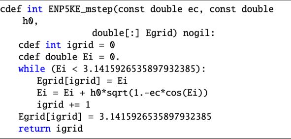
A.2.2 Function ENP5KE_coef
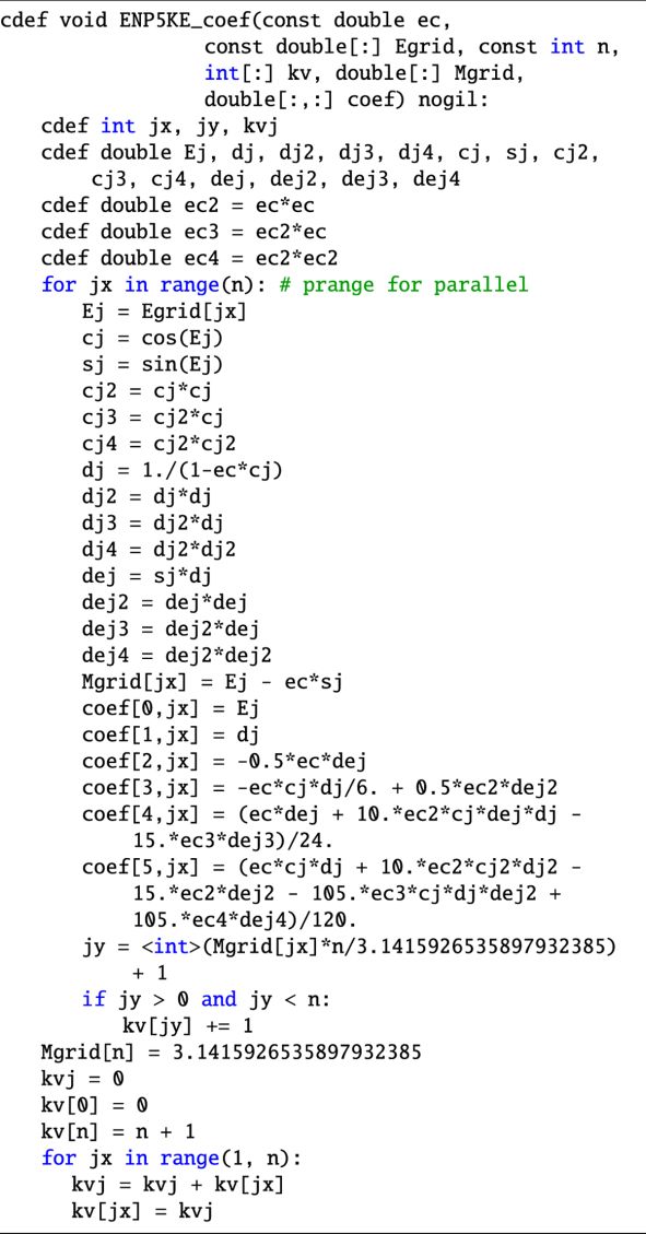
A.2.3 Function ENP5KE_evaluate
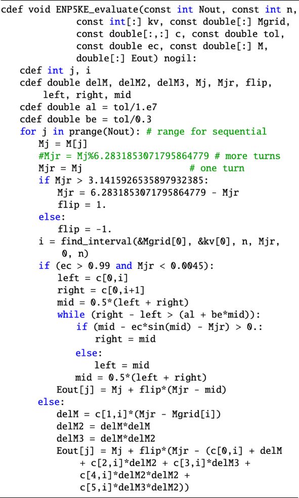
As discussed in Sect. 3.2, the ENP5KE_evaluate routine is so fast, that even one simple control sequence implying precomputed values has an appreciable effect on the execution time. Therefore, in the case e ≤ 0.99, the user may replace the bottom part, starting from the line “if (ec > 0.99 and Mjr < 0.0045):" to the end, with just
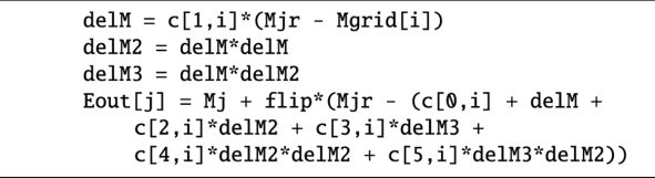
A.2.4 Function find_interval
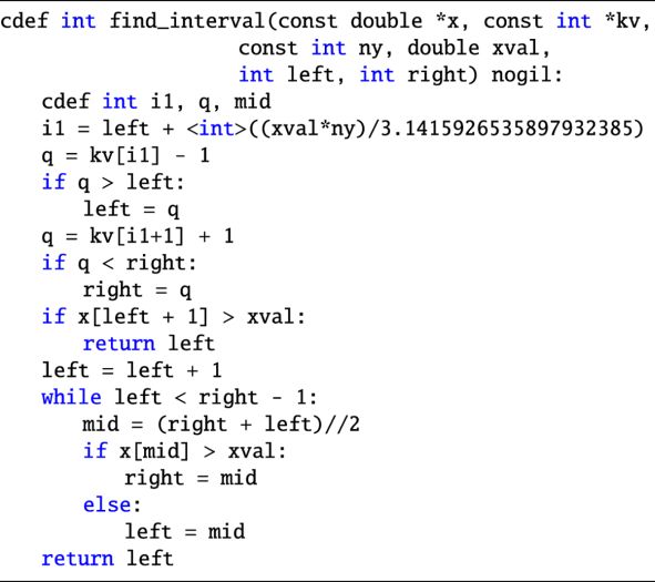
A.2.5 Wrapper class ENP5KE
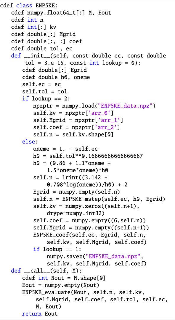
A.3 Routines for the ENMAKE method
The ENRKE routines given in Appendix A.1 can be modified to enhance Markley’s solver as discussed in Section 4. The ENMAKE_evaluate funtion is listed below.
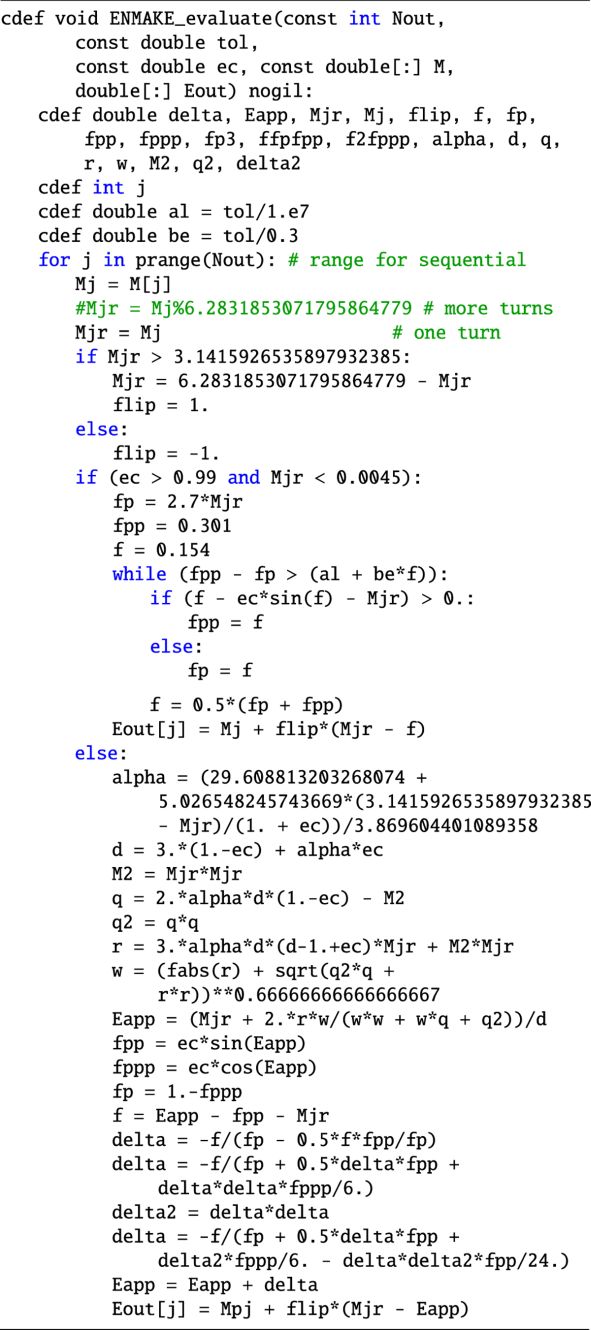
The wrapper class given for the ENRKE in Appendix A.1.2 can also be used for the ENMAKE method, uncommenting the call to ENMAKE_evaluate.
Appendix B Description of Cython Code and Routines
The motivation for using a high-level, interpreted object oriented language such as Python for numerical computation tasks are diverse. Examples include the following principal characteristics: lack of strong typing and type-checking, reduced syntax for rapid prototyping,lack of explicit pointers and explicit dynamic memory management, and easy inclusion and interoperability of a large collection of libraries. The cost, however, of directly using interpreted languages such as Python is performance. In recent years, several viable solutions have matured that allow critical sections or entire Python codes to be run with performance comparable (or better than) programs written in pure C/C++ or Fortran. These solutions come in two classes: JIT, or "Just in Time" execution (candidates such as PyPY or Numba), or code translation for compilation (such as Cython, C-API or others).
Here, we employed Cython for obtaining exceptional performance that is equal or better than the performance that would be obtained in pure C/C++. The performance could be better since hand-crafted C/C++ would require considerable skill to take advantage of low-level vectorization routines.
Below, we present the Cython implementations of the algorithms described in the text and in Appendix A. These routines contain the option of utilizing parallel execution for multicore CPUs. Informally, the Cython routines is essentially Python, but with directives, explicit variable typing, and typing of function calls. With these modifications, a library routine is used for translating the Cython code into a pure C programming code that is subsequently compiled. Once compiled, these routines provide high performance, optimized C codes that can be imported into Python scripts, used interactively, or used within an interactive Python notebook.
It should be mentioned that the C code that has been converted from the Cython code (in a processes often referred to as "cythonize"), consists of C-API directives. That is, every function that appears in the Python language has its C- equivalent. The cythonize operation converts cython codes into C code with calls to these C-API functions.
B.1 Compiling Cython: setup
The step needed to convert the Cython code into C and build an executable by linking to the required libraries is handled in the setup.py file. Namely, both the disutils and the Cython packages are needed for importing the explicit functions:
from distutils.core import setup
from distutils.extension import Extension
from Cython.Distutils import build_ext
from Cython.Build import cythonize
The next step is to call the distool setup function, which takes several parameters, including the name of the shared object module that will be built, the command to be executed, libraries to be used in the compilation, and the specification of the C include directories. To specify the libraries and compile arguments (for gcc or other), the Extension class is used.
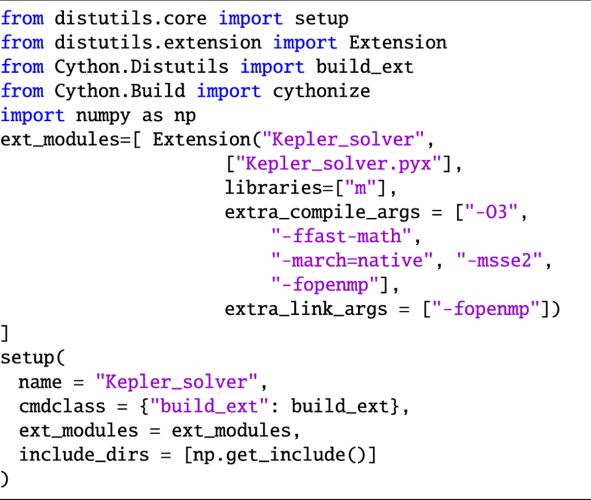
For compiling our code, the standard math library is used (specified by m, to signify that libm will be used. Next, we specify several optimization arguments for gcc, including the O3 optimization. Noticeable improvements are obtained with certain CPU architectures (in our case Intel i7) by using "-ffast-math", "-march=native", "-msse2". Finally, we include the OpenMP parallelization option for Cython using the Numerical optimization \verb|"-fopenmp"|.
B.2 Makefile
The setup.py can be invoked on the command line. We often use a simple Makefile for version control and ease of use. A minimal Makefile is given here (include the following in a file called Makefile):

Therefore, to compile the Cython code, the user only needs to execute:
make
on the command line, so that without tag arguments, the all block will be executed. This will create a shared object in the directory that can be imported into a python script.
Some details of the Cython syntax are worth commenting. The following listing shows the imports that we used in our routines.
B.3 Decorators
Because Cython is not typed and memory management is not explicitly handled by the user, some standard checks are incorporated into Python that add extra overhead. With respect to arrays, two checks are made for all array operations: bound checking and wraparound checks. The bound checking determines if an index is out of allocated memory assignment, while the wraparound deals with the fact that python arrays conceptually exist on a circle, and therefore can be accessed with negative indices, effectively wrapping around from the index i = 0 to i = n. Since such wraparound checks are unnecessary in C, and memory allocation errors are captured by memory management, these Python checks can be disabled. If invoked with a decorator functions before a function call, all the code within the function is subject to the condition specified.
Below are the decorators that we use for our routines.
If no other information and directives are included from a normal Python code to a Cython code, the translation to C is still possible. In fact, the resulting executable will be faster than the Python code. However, such conversions are not optimal, since the cythonize operation lacks specific information about variable and function return types. As a result, extra overhead code must be used to fix this at runtime. To mitigate this overhead and produce cleaner C code, explicit type information can and should be defined in Cython code.
In the following code, the cdef directive is required prefix followed by the explicit variable or function return type. Function arguments are also typed, but without the need for the cdef directive, since it is understood.
There are two other features of the above code that greatly affect the performance of the Cython routines: memoryview and the use of nogil. Control of these two constructs is fundamental for obtaining the best performance.
Memory view is the internal representation of one and multi dimensional arrays. While other idioms for memory allocation, such as the C style stdlib’s malloc, can be used, we found that the memoryview idiom is the most efficient. We also try to avoid conversion between numpy and memoryview whenever possible.
In concurrent multithreading contexts (such as the Linux/Unix kernel and other modern operating systems), thread synchronization mechanisms that protect independent program execution, can produce significant performance overhead and latency. One protection mechanism often employed is mutex locks. A mutex lock will block all threads from executing a critical section except one, thereby rendering multithreaded code single threaded. Because deadlocks can occur between threads accessing the Python interpretor, a global mutex lock is used, called the GIL, or global interpreter lock. In this case, the locking mechanism permits only one thread to execute the Python interpreter bytecode at a time. For the typical use case, the performance overhead of the GIL can be acceptable. However, in cases as presented here, the highest performance is required. Since the Python code will be translated to C/C++ native code and compiled with thread-safe libraries for multicore execution, the GIL can be disabled for this translation. This is done with the Cython directive nogil.
References
- Borsato, L., Marzari, F., Nascimbeni, V., et al. 2014, A&A, 571, A38 [NASA ADS] [CrossRef] [EDP Sciences] [Google Scholar]
- Boyd, J. P. 2015, Comput. Phys. Commun., 196, 13 [NASA ADS] [CrossRef] [Google Scholar]
- Brady, M. T., Petigura, E. A., Knutson, H. A., et al. 2018, ApJ, 156, 147 [Google Scholar]
- Brent, R. P. 1973, Algorithms for Minimization without Derivatives (Englewood Cliffs, NJ: Prentice-Hall) [Google Scholar]
- Calvo, M., Elipe, A., Montijano, J. I., & Randez, L. 2013, Celest. Mech. Dyn. Astron., 115, 143 [NASA ADS] [CrossRef] [Google Scholar]
- Ciceri, S., Lillo-Box, J., Southworth, J., et al. 2015, A&A, 573, L5 [NASA ADS] [CrossRef] [EDP Sciences] [Google Scholar]
- Colwell, P. 1993, Solving Kepler’s Equation Over Three Centuries (Richmond, VA: Willmann-Bell Inc.) [Google Scholar]
- Conway, B. A. 1986, Celest. Mech., 39, 199 [NASA ADS] [CrossRef] [Google Scholar]
- Danby, J., & Burkardt, T. 1983, Celest. Mech., 31, 95 [NASA ADS] [CrossRef] [Google Scholar]
- Eastman, J. D., Rodriguez, J. E., Agol, E., et al. 2019, PASP, submitted [arXiv:1907.09480] [Google Scholar]
- Elipe, A., Montijano, J. I., Randez, L., & Calvo, M. 2017, Celest. Mech. Dyn. Astron., 129, 415 [NASA ADS] [CrossRef] [Google Scholar]
- Farnocchia, D., Cioci, D., & Milani, A. 2013, Celest. Mech. Dyn. Astron., 116, 21 [NASA ADS] [CrossRef] [Google Scholar]
- Feinstein, S., & McLaughlin, C. 2006, Celest. Mech. Dyn. Astron., 96, 49 [NASA ADS] [CrossRef] [Google Scholar]
- Ford, E. B. 2006, ApJ, 642, 505 [Google Scholar]
- Fukushima, T. 1997, Celest. Mech. Dyn. Astron., 66, 309 [NASA ADS] [CrossRef] [Google Scholar]
- Gerlach, J. 1994, SIAM Rev., 36, 272 [CrossRef] [Google Scholar]
- Gooding, R. H., & Odell, A. W. 1988, Celest. Mech., 44, 267 [NASA ADS] [CrossRef] [Google Scholar]
- Gregory, P. C. 2010, MNRAS, 410, 94 [Google Scholar]
- Higham, N. J. 2002, Accuracy and Stability of Numerical Algorithms, 2nd edn. (USA: Society for Industrial and Applied Mathematics) [CrossRef] [Google Scholar]
- Kane, S. R., Ciardi, D. R., Gelino, D. M., & von Braun, K. 2012, MNRAS, 425, 757 [Google Scholar]
- Leleu, A., Alibert, Y., Hara, N. C., et al. 2021, A&A, 649, A26 [NASA ADS] [CrossRef] [EDP Sciences] [Google Scholar]
- López, R., Hautesserres, D., & San-Juan, J. F. 2017, MNRAS, 473, 2583 [Google Scholar]
- Makarov, V. V., & Veras, D. 2019, ApJ, 886:127, 1 [NASA ADS] [CrossRef] [Google Scholar]
- Markley, F. 1995, Celest. Mech. Dyn. Astron., 63, 101 [NASA ADS] [CrossRef] [Google Scholar]
- Mills, S. M., Howard, A. W., Petigura1, E. A., Fulton, B. J., & Weiss, H. I. L. M. 2019, ApJ, 157, 198 [Google Scholar]
- Mortari, D., & Elipe, A. 2014, Celest. Mech. Dyn. Astron., 118, 1 [NASA ADS] [CrossRef] [Google Scholar]
- Mortari, D., & Neta, B. 2000, Adv. Astron. Sci., 105, 449 [Google Scholar]
- Mortari, D., & Rogers, J. 2013, J. Astronaut. Sci., 60, 686 [NASA ADS] [CrossRef] [Google Scholar]
- Moshier, S. L. 2000, Cephes Math Library, Version 2.8, see http://www.moshier.net [Google Scholar]
- Odell, A. W., & Gooding, R. H. 1986, Celest. Mech., 38, 307 [NASA ADS] [CrossRef] [Google Scholar]
- Palacios, M. 2002, J. Comput. Appl. Math., 138, 335 [NASA ADS] [CrossRef] [Google Scholar]
- Prussing, J. E., & Conway, B. A. 2012, Orbital Mechanics, 2nd edn. (Oxford: Oxford University Press) [Google Scholar]
- Raposo-Pulido, V., & Pelaez, J. 2017, MNRAS, 467, 1702 [NASA ADS] [Google Scholar]
- Raposo-Pulido, V., & Pelaez, J. 2018, A&A, 619, A129 [NASA ADS] [CrossRef] [EDP Sciences] [Google Scholar]
- Roy, A. E. 2005, Orbital Motion, 4th edn. (Bristol and Philadelphia: Institute of Physics Publishing) [Google Scholar]
- Sartoretti, P., & Schneider, J. 1999, A&AS, 134, 553 [NASA ADS] [CrossRef] [EDP Sciences] [Google Scholar]
- Serafin, R. A. 1986, Celest. Mech., 38, 111 [NASA ADS] [CrossRef] [Google Scholar]
- Sotiriadis, S., Libert, A.-S., Bitsch, B., & Crida, A. 2017, A&A, 598, A70 [NASA ADS] [CrossRef] [EDP Sciences] [Google Scholar]
- Stumpff, K. 1968, National Aeronautics and Space Administration, Technical Note D-4460 [Google Scholar]
- Süli, E., & Mayers, D. 2003, An Introduction to Numerical Analysis (Cambridge: Cambridge University Press) [CrossRef] [Google Scholar]
- Tommasini, D. 2021, Mathematics, 9, 785 [Google Scholar]
- Tommasini, D., & Olivieri, D. N. 2020a, Appl. Math. Comput., 364, 124677 [Google Scholar]
- Tommasini, D., & Olivieri, D. N. 2020b, Mathematics, 8, 2017 [Google Scholar]
- Tommasini, D., & Olivieri, D. N. 2021, MNRAS, 506, 1889 [NASA ADS] [CrossRef] [Google Scholar]
- Worden, S. P., Drew, J., Siemion, A., et al. 2017, Acta Astron., 139, 98 [NASA ADS] [CrossRef] [Google Scholar]
- Zechmeister, M. 2018, A&A, 619, A128 [NASA ADS] [CrossRef] [EDP Sciences] [Google Scholar]
- Zechmeister, M. 2021, MNRAS, 500, 109 [Google Scholar]
- Zotos, E. E., Érdi, B., & Saeed, T. 2021, A&A, 645, A128 [NASA ADS] [CrossRef] [EDP Sciences] [Google Scholar]
All Tables
All Figures
|
Fig. 1 M dependence of the errors of the ENP5KE algorithm for solving KE in double precision for e = 0.8 (left) and e = 0.99 (right), when the input accuracy (tol) is set to the level 3 × 10⁻⁹ rad (top), 3 × 10⁻¹² rad (center), and 3 × 10⁻¹⁵ (bottom). For these values of e, the solutionis obtained using the piecewise quintic polynomial only, without the need for continuous bisection root search. |
| In the text | |
|
Fig. 2 M dependence of the errors of the ENP5KE algorithm for solving KE in double precision for e = 0.999 (left) and e = 1 − ϵ (right), when the input accuracy (tol) is set to the level 3 × 10⁻⁹ rad (top), 3 × 10⁻¹² rad (center),and 3 × 10⁻¹⁵ (bottom). For these values of e, the solution is obtained using the piecewise quintic polynomial for 0.0045 rad ≤ M ≤ 2π − 0.0045 rad, and with breakpoint bracketing followed by continuous bisection root search in the intervals M < 0.0045 rad and M > 2π − 0.0045 rad. |
| In the text | |
Current usage metrics show cumulative count of Article Views (full-text article views including HTML views, PDF and ePub downloads, according to the available data) and Abstracts Views on Vision4Press platform.
Data correspond to usage on the plateform after 2015. The current usage metrics is available 48-96 hours after online publication and is updated daily on week days.
Initial download of the metrics may take a while.