| Issue |
A&A
Volume 657, January 2022
|
|
|---|---|---|
| Article Number | A83 | |
| Number of page(s) | 10 | |
| Section | Cosmology (including clusters of galaxies) | |
| DOI | https://doi.org/10.1051/0004-6361/202141994 | |
| Published online | 18 January 2022 | |
Galaxy cluster strong lensing cosmography
Cosmological constraints from a sample of regular galaxy clusters⋆
1
Max-Planck-Institut für Astrophysik, Karl-Schwarzschild-Str. 1, 85748 Garching, Germany
e-mail: This email address is being protected from spambots. You need JavaScript enabled to view it.
2
Technische Universität München, Physik-Department, James-Franck Str. 1, 85741 Garching, Germany
3
Institute of Astronomy and Astrophysics, Academia Sinica, 11F of ASMAB, No. 1, Section 4, Roosevelt Road, Taipei 10617, Taiwan
4
Dipartimento di Fisica, Università degli Studi di Milano, Via Celoria 16, 20133 Milano, Italy
5
Dipartimento di Fisica e Scienze della Terra, Università degli Studi di Ferrara, Via Saragat 1, 44122 Ferrara, Italy
6
INAF – Osservatorio Astronomico di Bologna, Via Gobetti 93/3, 40129 Bologna, Italy
Received:
9
August
2021
Accepted:
15
October
2021
Abstract
Cluster strong lensing cosmography is a promising probe of the background geometry of the Universe and several studies have emerged thanks to the increased quality of observations using space- and ground-based telescopes. For the first time, we used a sample of five cluster strong lenses to measure the values of cosmological parameters and combine them with those from classical probes. In order to assess the degeneracies and the effectiveness of strong-lensing cosmography in constraining the background geometry of the Universe, we adopted four cosmological scenarios. We found good constraining power on the total matter density of the Universe (Ωm) and the equation of state of the dark energy parameter w. For a flat wCDM cosmology, we found Ωm = 0.30−0.11+0.09 and w = −1.12−0.32+0.17 from strong lensing only. Interestingly, we show that the constraints from the cosmic microwave background (CMB) are improved by factors of 2.5 and 4.0 on Ωm and w, respectively, when combined with our posterior distributions in this cosmological model. In a scenario where the equation of state of dark energy evolves with redshift, the strong lensing constraints are compatible with a cosmological constant (i.e. w = −1). In a curved cosmology, our strong lensing analyses can accommodate a large range of values for the curvature of the Universe of Ωk = 0.28−0.21+0.16. In all cosmological scenarios, we show that our strong lensing constraints are complementary and in good agreement with measurements from the CMB, baryon acoustic oscillations, and Type Ia supernovae. Our results show that cluster strong lensing cosmography is a potentially powerful probe to be included in the cosmological analyses of future surveys.
Key words: cosmology: observations / cosmological parameters / dark energy / gravitational lensing: strong / galaxies: clusters: general
Cosmological parameters posterior distributions are only available at the CDS via anonymous ftp to cdsarc.u-strasbg.fr (130.79.128.5) or via http://cdsarc.u-strasbg.fr/viz-bin/cat/J/A+A/657/A83
© G. B. Caminha et al. 2022
 Open Access article, published by EDP Sciences, under the terms of the Creative Commons Attribution License (https://creativecommons.org/licenses/by/4.0), which permits unrestricted use, distribution, and reproduction in any medium, provided the original work is properly cited.
Open Access funding provided by Max Planck Society.
1. Introduction
Cosmological observations suggest that the Universe is mostly composed of somewhat unconventional components whose nature is still not fully understood. Observations of the cosmic microwave background (CMB, Smoot et al. 1992; Hinshaw et al. 2013; Planck Collaboration VI 2020), baryon acoustic oscillations (BAO, Efstathiou et al. 2002; Eisenstein et al. 2005; DES Collaboration 2021), and Type Ia supernovae (SNe, Riess et al. 1998; Perlmutter et al. 1999; Astier et al. 2006; Scolnic et al. 2018) indicate that the evolution of the Universe at large scales (> 1 Mpc) is well described by the concordance Λ cold dark matter (ΛCDM) model. These ‘classical’ probes converge to a scenario where baryonic and CDM accounts for ≈30% of the energy density of the Universe. The remaining ≈70% is composed of dark energy associated with the cosmological constant Λ, and the Universe geometry must be very close to flat, that is with a vanishing curvature (Ωk ≈ 0).
However, deviations from these values and different models describing the dark energy can be accommodated by the current data, see for example Motta et al. (2021) for a recent review. Moreover, at smaller scales, the flat ΛCDM model has difficulties to explain some properties related to structure formation, for instance the sub-halo population in galaxy clusters (Grillo et al. 2015; Carlsten et al. 2020; Meneghetti et al. 2020) and the inner slope of dark matter halos (Sand et al. 2004; Gnedin et al. 2004, 2011; Newman et al. 2011, 2013a,b; Martizzi et al. 2012; Schaller et al. 2015), when comparing simulations with observations. These issues motivate further tests on the ΛCDM model, both at small and large scales, and they play an essential role in the concept and design of cosmological observations and projects, such as the Baryon Oscillation Spectroscopic Survey (Dawson et al. 2013), the Dark Energy Survey (Abbott et al. 2018; DES Collaboration 2021; Porredon et al. 2021), the Kilo-Degree Survey (van Uitert et al. 2018; Joudaki et al. 2018), and the Planck satellite (Planck Collaboration VI 2020), to mention a few.
Strong gravitational lensing, among many other applications in astrophysics (see e.g. Schneider et al. 1992; Kneib & Natarajan 2011), can also be used to probe the background geometry of the Universe. On galaxy scales, significant progress has been made in the last decade in order to increase the accuracy of lens modelling and thus to obtain precise measurements of some relevant cosmological parameters (see e.g. Suyu et al. 2010; Chen et al. 2019; Wong et al. 2020; Shajib et al. 2020; Birrer et al. 2020). In these systems, the primary sensitivity is on the Hubble constant from the measurements of time delays between multiple images of the same source, especially of strongly lensed quasars (e.g. Fassnacht et al. 2002; Courbin et al. 2018; Millon et al. 2020a,b). Although measurements of the values of Ωm and Ωk are also possible when the lens galaxy dynamical data are available (Grillo et al. 2008; Cao et al. 2012) or when two or more sources at different redshifts are multiply lensed (Collett & Auger 2014; Smith & Collett 2021), they are either observationally expensive or rare and they are prone to intrinsic mass-sheet degeneracies because of the small number of multiply lensed sources (Schneider 2014).
In contrast, massive galaxy clusters can generate dozens of multiple images from sources in a large interval of redshifts. Because of that, they are excellent systems to probe Ωm, Ωk, and also the equation of state parameter w of the dark energy. Cluster strong lensing cosmography has been discussed in the past (Blandford & Narayan 1992); however, it requires high-quality data, more specifically, high-resolution imaging and deep spectroscopy to identify and measure redshifts of a large number of multiple images. The possibility of constraining cosmological parameters with this methodology was explored in more detail in subsequent works using simulated data (Link & Pierce 1998; Golse et al. 2002; Gilmore & Natarajan 2009; D’Aloisio & Natarajan 2011). It was only with the combination of imaging with the Hubble Space Telescope (HST) and extensive spectroscopy from different instruments in the field of the galaxy cluster Abell 1689 that the first competitive cosmological constraints were obtained in Jullo et al. (2010). Moreover, a collection of models of dark energy with different equations of state was studied using the constraints from Abell 1689 (Magaña et al. 2015, 2018). Later, with the deployment of the Multi Unit Spectroscopic Explorer (MUSE; Bacon et al. 2014) at the Very Large Telescope (VLT), the number of spectroscopically confirmed multiple images in clusters has increased significantly (see e.g. Richard et al. 2015; Grillo et al. 2016; Caminha et al. 2017a). Based on MUSE spectroscopy and HST data, in Caminha et al. (2016a) we have shown that the combination of a regular total mass distribution and a large number of multiple images with redshifts in the range of zsrc = [0.7 − 6.1] makes the cluster Abell S1063 an excellent system for cluster strong lensing cosmography. Finally, in Grillo et al. (2018, 2020), a similarly high-precision lens model of MACS J1149, which is one of the very few galaxy clusters with measured time delays between the multiple images of a time-varying source, was used to measure the values of the Hubble constant, Ωm and ΩΛ.
Although the number of galaxy clusters with accurate strong lensing models has increased in recent years, a combined cosmographical analysis using a cluster sample has not been carried out yet. In addition to improving the figure of merit, the combination of different clusters is important to mitigate possible systematic effects that might affect the individual strong-lensing models in different ways, for instance, line-of-sight perturbers, intrinsic degeneracies in the models that depend on the cluster redshift and distribution of background sources, mass components external to the cluster cores, etc. In this work, we use a sample of five clusters, acting as strong lenses, with deep spectroscopy from MUSE and HST photometry from the Cluster Lensing And Supernova survey with Hubble (CLASH; Postman et al. 2012) with well studied lens models in the literature, including Abell S1063 that also belongs to the Hubble Frontier Fields (HFF; Lotz et al. 2017).
This paper is structured as follows. In Sect. 2 we present our cluster sample and some aspects of strong lens modelling. The methodology and the cosmological constraints from the lensing analyses are shown in Sect. 3, and the combination with other probes is explored in Sect. 4. Finally, in Sect. 5 we summarise our results and discuss future developments of this work.
2. Cluster sample and strong lensing models
In this work, we use clusters with strong lensing models based on-2pt extensive HST photometry and deep spectroscopy, mainly from VLT/MUSE. They are the CLASH ‘gold sample’ presented in Caminha et al. (2019), consisting of the clusters RX J2129, MACS J1931, MACS J0329, and MACS J2129. We have also included the HFF target Abell S1063, which has been shown to be a very efficient cluster for cosmography, given its combination of regular mass distribution and the high number of strong lensing constraints (see e.g. Caminha et al. 2016a). This sample of clusters has a redshift range of zlens ≈ [0.23 − 0.59] with a large number of multiple images. Thanks to dedicated spectroscopic follow-ups (Belli et al. 2013; Rosati et al. 2014; Caminha et al. 2016a,b, 2019; Huang et al. 2016; Karman et al. 2017; Monna et al. 2017), many multiple images have spectroscopic confirmation in the range zsrc ≈ [0.7 − 6.9], thus providing exceptional constraints to the strong lensing models. As pointed out by D’Aloisio & Natarajan (2011) and Acebron et al. (2017), this large redshift range is particularly important to reduce the biases and intrinsic degeneracies on the cosmological constraints obtained from strong lensing analyses, which we describe in Sect. 3. In our models, we use only families of multiple images with spectroscopic confirmation in order not to include any additional free parameter (i.e. the background source redshift) and to ensure we have not misidentified multiple images.
We modelled the mass distribution of our cluster sample using a superposition of parametric profiles. In detail, the cluster scale components were parameterised by pseudo-isothermal elliptical mass distributions (PIEMD, Kassiola & Kovner 1993). We also tested the Navarro-Frenk-White model (NFW, Navarro et al. 1996, 1997) to describe the cluster scale mass distribution, however these models are less accurate in predicting the multiple image positions in comparison to PIEMD models. In Appendix A, we discuss the best fit models using the NFW profile. The cluster members were modelled by dual pseudo-isothermal mass distributions with a vanishing core radius (Elíasdóttir et al. 2007; Suyu & Halkola 2010), and they follow a constant total mass-to-light ratio to reduce the number of free parameters. For more details on the observational data and the mass modelling of the cluster sample used in this paper, we refer readers to the works of Caminha et al. (2016a, 2019).
In Table 1, we list the degree of freedom (d.o.f. ≡ number of constraints – number of free parameters) and the number of free parameters (Nfree) for each cluster and the different cosmological models we consider in this work. Moreover, we also provide the root mean square (rms) of the differences between the model predicted and observed positions of the multiple images, and the reduced image-plane χ2. The models with fixed cosmology have from eight to 16 free parameters, a number that is relatively simple to sample with commonly used MCMC codes, for instance the bayeSys algorithm1 implemented in the lenstool software that we use (Kneib et al. 1996; Jullo et al. 2007; Jullo & Kneib 2009). We note that in some models, the presence of a second dark matter halo is favoured by the best-fitting models. However, these secondary components are located outside the strong lensing region, that is at projected distances from the cluster centre larger than ≳200 kpc, acting as perturbers and they are not the main contributors for the formation of multiple images used in this work.
Summary of the different strong lensing models.
Clusters with more complex total mass distributions, for instance merging systems or cases with prominent perturbers along the line-of-sight at different redshifts, demand an increased number of free parameters to predict the positions of all multiple images. This is the case of some HFF and CLASH clusters, such as MACS J0416, Abell 370, Abell 2744, MACS J1149, and MACS J1206 (Grillo et al. 2016; Caminha et al. 2017a,b; Mahler et al. 2018; Lagattuta et al. 2019; Bergamini et al. 2021; Richard et al. 2021). These clusters need from 21 to ≈40 free parameters to characterise their mass components, compared to fewer than 20 free parameters for the clusters in our sample indicated in Table 1. The high number of free parameters makes it challenging to sample the likelihood, especially the cosmological parameters that have a small impact on the multiple image positions. Moreover, the fact that they are merging systems and we use a combination of relatively simple parametric models might introduce a bias in our measurement of the cosmological parameters. One possibility is to explore more complex, or semi-parametric models (see e.g. Beauchesne et al. 2021) to describe such complex mass distributions. In this work, we focus on the sample of clusters with a regular mass distribution, and the cosmographical analyses of clusters with a more complex total mass distribution and/or in a merging state will be the subject of a future publication.
3. Strong lensing cosmological constraints
In this section we describe the methodology and assumptions we adopted in our cluster strong lensing models to probe the background cosmology of the Universe. The results of our strong lensing analyses, that is the constrained parameters and their posterior distributions, are presented at the end of this section.
3.1. Distance ratios from multiply lensed sources
Through its relation to the angular diameter distances, the strong lensing effect is affected by the background geometry of the Universe. The relation between the observed (θ) and intrinsic (β) positions of a lensed galaxy i is given by the so-called lens equation:
 (1)
(1)
where DL, Si and DO, Si are the angular diameter distances between the lens (L) and the background source (Si), and the observer (O) and the background source, respectively. The function α is the deflection angle and this quantity only depends on the projected total lens potential ψ(θ) of the deflector and the position of the lensed image via the relation α(θ)∝∇ψ(θ). From this equation, the ratio of the cosmological distances and the lens potential are degenerate through a multiplicative factor. However, in the case of more than one multiple-image family at different redshifts, this degeneracy is strongly reduced since the projected lens potential of the cluster is the same for all sources. Thus, the positions of the multiple images of two background sources Si and Sj provide information on the quantity
 (2)
(2)
For Ns background sources that are strongly lensed by the same cluster, we therefore obtain Ns − 1 independent distance ratios Ξij. The measurements of these Ξij then yield information on the background cosmology. Specifically in our cluster sample, the number of multiply lensed background sources used as input in the lens models are 7, 20, 7, 9, and 11 for RXJ 2129, Abell S1063, MACS J1931, MACS J0329, and MACS J2129, respectively.
3.2. Cosmological models
We consider four different cosmological models to assess the degeneracies and the effectiveness of strong-lensing cosmography in constraining the background geometry of the Universe. They are as follows:
-
Flat-ΛCDM cosmology is the simplest model adopted here. It is a flat Universe where only Ωm varies and the other parameters are fixed (w = −1, wa = 0, and Ωk = 0).
-
Flat-wCDM is also a flat cosmology in which the dark energy equation of state parameter (w ≡ P/ρ) is allowed to vary, but it does not depend on redshift (i.e. wa = 0).
-
Curved-ΛCDM is a cosmological model with free curvature and a fixed equation of state of dark energy (w = −1).
-
CPL cosmology consists of a flat Universe where the dark energy equation of state can vary with redshift using a Chevallier-Polarski-Linder parametrisation (CPL, Chevallier & Polarski 2001; Linder 2003) given by:
 (3)
(3)
Moreover, we adopted flat priors for the values of the cosmological parameters, allowing them to vary in the ranges:
![Mathematical equation: $$ \begin{aligned}&\Omega _{\rm m} = [0,1], \end{aligned} $$](/articles/aa/full_html/2022/01/aa41994-21/aa41994-21-eq8.gif) (4)
(4)
![Mathematical equation: $$ \begin{aligned}&\Omega _\Lambda = [0,1], \end{aligned} $$](/articles/aa/full_html/2022/01/aa41994-21/aa41994-21-eq9.gif) (5)
(5)
![Mathematical equation: $$ \begin{aligned}&w\,(\mathrm{or}\,w_0) = [-3, 0], \end{aligned} $$](/articles/aa/full_html/2022/01/aa41994-21/aa41994-21-eq10.gif) (6)
(6)
![Mathematical equation: $$ \begin{aligned}&w_{\rm a} = [-3,3]. \end{aligned} $$](/articles/aa/full_html/2022/01/aa41994-21/aa41994-21-eq11.gif) (7)
(7)
We note that in lenstool, the curvature is parameterised by the parameter ΩΛ and the results here are presented in terms of Ωk, converted with the linear relation Ωk = 1 − Ωm − ΩΛ.
3.3. Lens modelling
In order to obtain the cosmological constraints with our strong lensing models, we first obtained the best-fit parameters for each model (see Table 1) considering a positional error on the multiple image positions of  , and, in a second step, we ran lenstool to sample the posterior distribution of the free parameters. To secure sensible confidence intervals for the values of the parameters (i.e. error bars), we re-scaled the positional errors in order to have χ2/d.o.f. = 1 in the sampling runs. The values of the re-scaled errors are similar to those of the rms of each model and range from
  to
to  . With this, we account for effects that are not included in the modelling, such as line-of-sight mass structures (Jullo et al. 2010; Host 2012), possible deviations of some cluster members from the adopted scaling relations and asymmetries in the cluster scale component that are not represented by simple elliptical models well. We left the chains running until they reached at least 106 points for all models and, in the case of the CPL cosmology that has three free cosmological parameters (Ωm, w0, wa), we allowed for a longer run to obtain a minimum of 2 × 10⁶ points to properly sample the parameter space. We note that in all models, the Gelman-Rubin convergence test (Brooks & Gelman 1998) results in values lower than 1.1 for all free parameters, which ensures that the chains have reached convergence.
In total, we sampled the parameter space of 20 independent models for all five clusters in the four different cosmological models. From the MCMC chains, we computed the probability distribution functions (PDFs) of the cosmological parameters, and the combined constraints were obtained by multiplying the PDFs of each cluster of a specific cosmology, that is,
 (8)
(8)
where five is the number of clusters we use in this work, j refers to one of the four adopted cosmologies, and Pi is the PDF of cluster i marginalised over its total mass parameters. When combining this with other cosmological observables (see Sect. 4), the function  is further multiplied with the PDFs from the additional probes. To obtain the constrained values of each cosmological parameter, we projected the combined PDF in the corresponding direction and computed the median value and confidence interval of the one-dimensional distribution.
3.4. Cosmological constraints from lensing clusters
In Fig. 1, we show the PDFs of the flat-ΛCDM cosmological model for each cluster in different colours. The single PDFs are somewhat broad, with a 68% confidence level interval of the order of ≈0.2 − 0.4. Despite having a relatively small model rms (see Table 1), we note that the PDF of RX J2129 seems to overestimate the value of Ωm when comparing it to the other clusters, but with a long tail towards low values. This might be due to the fact that the multiple images are located within a very small region of the cluster core (< 100 kpc), and their redshift interval is zsrc = [0.68 − 3.43], whereas the other clusters have at least one multiple image family at zsrc > 5. The more restricted source redshift range in RX J2129 results in larger uncertainties on Ωm, and the higher Ωm value is statistically consistent with those of the other clusters within 2σ2. Therefore, the combined constraint is not significantly affected by this cluster. From Table 1, the changes to the values of the best-fit rms and reduced χ2 are very small. This indicates that the model with fixed cosmology (i.e. Ωm = 0.3) is already close to the actual value; thus Ωm has a slight impact on the best-fit models. When combining all clusters, however, we obtained a narrower constraint of  .
.
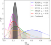 |
Fig. 1. One-dimensional PDFs for the flat-ΛCDM cosmology, where only the value of Ωm varies. Strong lensing constraints of each cluster are shown in different colours. Filled regions indicate the 68% confidence intervals. The grey curve shows the combined constraints from all five clusters. Values and combination with other cosmological probes are presented in Table 2. |
In the left panel of Fig. 2, we show the 68% confidence regions for the parameters Ωm and w in the flat-wCDM scenario (i.e. Ωk = 0). Similar to Fig. 1, the constraints from individual clusters are relatively wide, except for Abell S1063. As we mentioned before and as discussed in Caminha et al. (2016a), this cluster has a remarkably regular shape in combination with a large number of spectroscopically confirmed multiple images. Moreover, the intrinsic degeneracies between these two cosmological parameters change with respect to the lens redshift through the distance ratio constraints in Eq. (2). Lenses at lower redshifts tend to have an extended ‘tail’ towards higher values of Ωm for low values of w (see, e.g. RX J2129 and MACS J1931), forming an inverted L-shaped constraint in the w − Ωm plane. Such an L-shaped degeneracy is less pronounced for higher-redshift clusters, such as MACS J0329 and MACS J2129. In this cosmology, the strong lensing combined constraints (median and 68% confidence levels) are  and
and  (see Table 2).
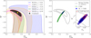 |
Fig. 2. Cosmological constraints for the flat-wCDM cosmological model, where Ωm and w are free parameters. Left panel: 68% confidence levels from the strong lensing analyses for each cluster (coloured regions) and the combined constraint shown by the grey region. The yellow circle shows the median value of the constrained cosmological parameters (see Table 2). Right panel: combination with other cosmological observables. The inset box shows the additional combination with BAO and SN. The contours indicate the 68% and 95% confidence regions. The strong lensing confidence levels are almost perpendicular to those obtained from the CMB and when combined, strong lensing improves the CMB constraints by factors of 2.5 and 4.0 on Ωm and w, respectively. |
Summary of the cosmological constraints.
We also explore the possibility of constraining the curvature of the Universe with our strong lens models. In order to maintain the number of free parameters describing the curved-ΛCDM cosmology, we fixed the value w = −1 and varied those of Ωm and Ωk. In the left panel of Fig. 3, we show the strong lensing constraints on these two parameters. Through our prior range, regions of nonphysical values of ΩΛ are excluded (see Sect. 3.2) and indicated in the figure. In this scenario, the combined constraint on the dark matter density parameter is  . The median value is somewhat larger when comparing it with the flat-wCDM cosmology, but it is consistent within the 68% confidence interval. On the other hand, the curvature is not strongly constrained and our models provide a relatively large interval,
  . Although large, these constraints on Ωk are still complementary to those from other cosmological probes, as we discuss in Sect. 4.
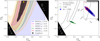 |
Fig. 3. Same as Fig. 2, but for the curved-ΛCDM cosmology, with fixed w = −1 and free Ωm and Ωk. Regions outside our priors on ΩΛ (i.e. ΩΛ < 0 or > 1) were not sampled and indicated in the panels. Although strong lensing only does not obtain stringent constraints on the curvature parameter, it is still complementary to other probes due to its perpendicular parameter degeneracies with respect to the CMB. |
Finally, in Fig. 4 we show the constraints on the three cosmological parameters of the CPL scenario from our models. Because of the additional free parameter wa (see Eq. (3)), the strong lensing constraints of each single cluster are wider and difficult to visualise. Thus, only the 68% confidence level of the combined constraints are shown in each two-dimensional projection of the three parameters. We note that the region where wa > −w0 was removed because it yields a Universe model dominated by dark energy at early times and this is excluded by high-redshift studies (see e.g. Wright 2007; Kowalski et al. 2008; Komatsu et al. 2011; Planck Collaboration VI 2020). In this scenario, we obtain the following constraints from the strong lensing only analyses:  ,
,  and
and  .
.
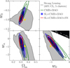 |
Fig. 4. Confidence levels for the CPL model. Here we show in grey the 68% confidence level for the strong-lensing-only analyses for better visualisation, and the yellow circle indicates the median values of Table 2. The 68% and 95% combined constraints of different probes are shown with coloured contours. The region where wa > −w0 was excluded because it produces a non-physical cosmology. In this cosmology with one additional free parameter, our strong lensing models are still capable of improving the constraints when combined to classical probes, especially on the parameters w0 and wa of the dark energy equation of state. |
In all cosmological scenarios, the values of Ωm are in agreement within the 68% confidence levels (see Table 2), although the size of this interval increases with the number of free cosmological parameters, as expected. Overall, the current precision of the lensing models, which is reached thanks to the deep spectroscopy available, provides meaningful constraints from the strong-lensing-only analyses. The combination and complementarity of our strong-lensing constraints with other observational probes is discussed in the following section.
4. Combination with other cosmological probes
To explore the full potential of our cluster-strong-lensing cosmological constraints, we combined our results with those from other probes in this section. In order to be consistent with previous works and quantify the improvement on the figure of merit of the combined constraints, we use the publicly available posterior distributions from the Planck Collaboration (Planck Collaboration VI 2020). Specifically, we consider the chains containing constraints from CMB plus lensing power spectrum reconstruction likelihood, since for the CPL cosmology, the CMB-only chain is not available. The other measurements come from Type Ia Supernovae (SNe) using the Pantheon sample (Scolnic et al. 2018), and BAO using results from the 6-degree Field Galaxy Survey and Sloan Digital Sky Survey Main Galaxy Sample (Carter et al. 2018) as well as a compilation of different analyses of the BOSS DR12 data (Ross et al. 2017; Beutler et al. 2017; Vargas-Magaña et al. 2018). We refer the reader to Sects. 5.1 and 5.2 of Planck Collaboration VI (2020) for more details on these additional probes.
In Table 2, we summarise the median and the 68% confidence levels of the cosmological parameters constrained from our combined strong lensing models only (SL), CMB, BAO, and SN, and their combinations. To quantify the improvement on the figure of merit from the incorporation of the strong lensing constraint, we define the quantity δi as the ratio between the 68% confidence interval of the cosmological parameter i, obtained from the constraints without and with strong lensing results.
For the flat-ΛCDM cosmology, the CMB-only constraints are very stringent compared to all other probes and they dominate the combined posterior distributions. Although the values of Ωm are consistent, the degeneracy between this parameter and the cluster mass distributions in the strong lensing models yields a relatively large statistical error. In this simple cosmology, there are no improvements on the figure of merit when including the strong lensing information on the combined probes (see the values of δΩm on Table 2). Nevertheless, considering models with additional free cosmological parameters, the strong lensing analyses add substantial constraints on the cosmological parameters.
The combined constraints for the flat-wCDM cosmology are shown in the right panel of Fig. 2, where the contours indicate the 68% and 95% confidence-level intervals. Interestingly, strong lensing and CMB have an almost perpendicular parameter degeneracy, and the combination of SL×CMB improves significantly over the individual constraints. The error bars on the parameters Ωm and w are reduced by factors of 2.5 and 4.0, respectively (see Table 2). Naturally, the improvement is minor in the case where the other three probes are combined, that is CMB×BAO×SN. However, the strong lensing information can still reduce the error bars by factors of ≈5%.
In the right panel of Fig. 3, we show the combined constraints for the curved-ΛCDM cosmological model. As discussed in the previous sections, cluster strong lensing is not very efficient in constraining the curvature of the Universe and provides a large error bar on this parameter. However, it still improves the constraints on Ωk when combined with the CMB. From Table 2, the figure of merit improves by a factor of ≈1.15 on both Ωm and Ωk when both observables are considered. When combining all observables, the improvements on Ωm are comparable to the flat-wCDM cosmology, but the constraint on Ωk is not affected. Such an effect is due to the large confidence region obtained from the strong lensing analyses (see both panels of Fig. 3) that tends to overestimate the value of the curvature of the Universe. The results from other probes, which indicate that the Universe is very close to being flat, and the weak constraining power on Ωk make cluster-strong-lensing cosmography not very efficient in probing this particular cosmological scenario.
For the CPL cosmology, the constraint from CMB only is not available in the public release from Planck Collaboration VI (2020) because of difficulties in the convergence of the posterior distribution. Therefore, we first combined the strong-lensing constraints with the CMB×BAO probes. In addition to the 68% confidence regions of the strong lensing analyses displayed in Fig. 4, we also show the 68% and 95% regions for the combined constraints. The combined SL×CMB×BAO constraints improve the error bars on the three parameters Ωm, wa and w0 by factors of ≈1.4 − 1.3 (see Table 2 for more details). Although the parameter degeneracies of all probes have similar directions in the wa − Ωm plane, the probes have good complementarity in the other two projections. In particular, high values of w0 allowed by the CMB×BAO probe are excluded by the strong lensing analyses. We note that our results are also in excellent agreement when including constraints from SN (see the last row of Table 2). All of these results demonstrate that cluster strong lensing cosmography can be used to constrain cosmological parameters and complement other standard probes.
5. Conclusions
In this work, we use galaxy cluster strong lenses to constrain the parameters of the background cosmology of the Universe for the first time using a sample of galaxy clusters. Thanks to the large number of multiple image families with spectroscopic redshifts, we are able to obtain competitive parameter constraints. In order to estimate the efficiency of strong lensing cosmography in constraining cosmological parameters, we adopted four different cosmologies. Moreover, we quantified the improvements when combining our posterior distributions with classical cosmological probes (i.e. CMB, BAO, and SN). Our main results are summarised as follows:
-
We used the strong lensing models of each cluster to obtain the posterior distributions of the cosmological parameters. The combined constraints using the strong lensing models are all in agreement with other probes. Only for the curvature of the Universe (Ωk) in the curved-ΛCDM model are the strong lensing constraints not stringent. Thus, cluster strong lensing cosmography is not efficient in probing the curvature parameter Ωk.
-
On the other hand, the strong lensing analyses provide stringent constraints on the dark energy equation of state parameters. In the case of a flat-wCDM cosmology, we obtain values of
 and
and  for the 68% confidence interval. The interval for the parameter w is comparable to the CMB constraints (see Table 2).
 -
For the flat-wCDM and CPL cosmologies, the strong lensing constraints on the equation of state for the dark energy component are consistent with the standard ΛCDM model (i.e. w or w0 = −1 and wa = 0) within the 68% confidence level. Even though the constraints on w0 are weak, the parameter degeneracies in the CPL cosmology have some complementarity with other probes, especially in the projections w0 − Ωm and w0 − wa (see Fig. 4).
-
When combining strong lensing and CMB constraints, we find that we can improve the figure of merit on the cosmological parameters by significant factors. In the flat-wCDM cosmology, the constraints on Ωm and w improve by factors of 2.5 and 4.0, respectively. For the curved-ΛCDM cosmology, the improvement is of the order of 1.15 in both Ωm and Ωk parameters. In the more complex CPL cosmological model, we combined the strong lensing posterior distributions with the CMB×BAO constraints, leading to an improvement of ≈1.4 − 1.3 on the three free parameters (Ωm, w0, and wa).
-
Finally, we find excellent agreement of our strong lensing analyses when comparing them to the three ‘classical’ probes (CMB, BAO, and SN) altogether. For the parameter Ωk, the combined constraint is not affected because strong lensing is weakly sensitive to this parameter. However, in all other cosmological models, we show that cluster strong lensing cosmography can be a complementary probe and contribute to the combined probes.
Here we perform these analyses using a sample of five cluster strong lenses because of our knowledge of these systems from previous detailed works. These cosmological constraints can be further improved by including new strong lensing models of additional clusters with similar data. For instance, the number of clusters with deep spectroscopy, mainly using MUSE, is constantly increasing (see e.g. Richard et al. 2021) and these will be included in future analyses.
Moreover, several cosmological surveys from the ground and space, such as the Rubin Observatory Legacy Survey of Space and Time (LSST, Ivezić et al. 2019), Euclid Space Telescope (Laureijs et al. 2011; Scaramella et al. 2021), and the Nancy Grace Roman Space Telescope (Spergel et al. 2015), will start to operate in the next few years. They will map most of the visible sky with unprecedented image quality and depth, and provide a large number of galaxy clusters that can be followed up with deep spectroscopy, increasing our sample of clusters by factors of tens and perhaps hundreds. With data from this upcoming generation of telescopes, we might also be able to discern among different cosmological models. Finally, we make the posterior distributions (in the format of parameter chains) of the cosmological and lens mass parameters obtained in this work publicly available.
With five clusters, it is statistically likely that one or two clusters would yield constraints that are not consistent within 1σ with the constraints from other clusters, but they are likely to be consistent within 2σ.
Acknowledgments
The authors thank the anonymous referee who provided useful suggestions that improved this manuscript. GBC and SHS acknowledge the Max Planck Society for financial support through the Max Planck Research Group for SHS and the academic support from the German Centre for Cosmological Lensing. CG and PR acknowledge financial support through grant PRIN-MIUR 2017WSCC32 ‘Zooming into dark matter and proto-galaxies with massive lensing clusters’ (P.I.: P. Rosati). This research made use of Astropy (http://www.astropy.org), a community-developed core Python package for Astronomy (Astropy Collaboration 2013, 2018), NumPy (Harris et al. 2020), Matplotlib (Hunter 2007) and GetDist (Lewis 2019).
References
- Abbott, T. M. C., Abdalla, F. B., Alarcon, A., et al. 2018, Phys. Rev. D, 98, 043526 [NASA ADS] [CrossRef] [Google Scholar]
- Acebron, A., Jullo, E., Limousin, M., et al. 2017, MNRAS, 470, 1809 [Google Scholar]
- Astier, P., Guy, J., Regnault, N., et al. 2006, A&A, 447, 31 [NASA ADS] [CrossRef] [EDP Sciences] [Google Scholar]
- Astropy Collaboration (Robitaille, T. P., et al.) 2013, A&A, 558, A33 [NASA ADS] [CrossRef] [EDP Sciences] [Google Scholar]
- Astropy Collaboration (Price-Whelan, A. M., et al.) 2018, AJ, 156, 123 [Google Scholar]
- Bacon, R., Vernet, J., Borisova, E., et al. 2014, The Messenger, 157, 13 [NASA ADS] [Google Scholar]
- Beauchesne, B., Clément, B., Richard, J., & Kneib, J.-P. 2021, MNRAS, 506, 2002 [NASA ADS] [CrossRef] [Google Scholar]
- Belli, S., Jones, T., Ellis, R. S., & Richard, J. 2013, ApJ, 772, 141 [NASA ADS] [CrossRef] [Google Scholar]
- Bergamini, P., Rosati, P., Vanzella, E., et al. 2021, A&A, 645, A140 [EDP Sciences] [Google Scholar]
- Beutler, F., Seo, H.-J., Saito, S., et al. 2017, MNRAS, 466, 2242 [Google Scholar]
- Birrer, S., Shajib, A. J., Galan, A., et al. 2020, A&A, 643, A165 [NASA ADS] [CrossRef] [EDP Sciences] [Google Scholar]
- Blandford, R. D., & Narayan, R. 1992, ARA&A, 30, 311 [NASA ADS] [CrossRef] [Google Scholar]
- Brooks, S. P., & Gelman, A. 1998, J. Comput. Graph. Stat., 7, 434 [Google Scholar]
- Caminha, G. B., Grillo, C., Rosati, P., et al. 2016a, A&A, 587, A80 [NASA ADS] [CrossRef] [EDP Sciences] [Google Scholar]
- Caminha, G. B., Karman, W., Rosati, P., et al. 2016b, A&A, 595, A100 [NASA ADS] [CrossRef] [EDP Sciences] [Google Scholar]
- Caminha, G. B., Grillo, C., Rosati, P., et al. 2017a, A&A, 600, A90 [NASA ADS] [CrossRef] [EDP Sciences] [Google Scholar]
- Caminha, G. B., Grillo, C., Rosati, P., et al. 2017b, A&A, 607, A93 [NASA ADS] [CrossRef] [EDP Sciences] [Google Scholar]
- Caminha, G. B., Rosati, P., Grillo, C., et al. 2019, A&A, 632, A36 [NASA ADS] [CrossRef] [EDP Sciences] [Google Scholar]
- Cao, S., Pan, Y., Biesiada, M., Godlowski, W., & Zhu, Z.-H. 2012, JCAP, 2012, 016 [CrossRef] [Google Scholar]
- Carlsten, S. G., Greene, J. E., Peter, A. H. G., Greco, J. P., & Beaton, R. L. 2020, ApJ, 902, 124 [NASA ADS] [CrossRef] [Google Scholar]
- Carter, P., Beutler, F., Percival, W. J., et al. 2018, MNRAS, 481, 2371 [NASA ADS] [CrossRef] [Google Scholar]
- Chen, G. C. F., Fassnacht, C. D., Suyu, S. H., et al. 2019, MNRAS, 490, 1743 [NASA ADS] [CrossRef] [Google Scholar]
- Chevallier, M., & Polarski, D. 2001, Int. J. Mod. Phys. D, 10, 213 [Google Scholar]
- Collett, T. E., & Auger, M. W. 2014, MNRAS, 443, 969 [NASA ADS] [CrossRef] [Google Scholar]
- Courbin, F., Bonvin, V., Buckley-Geer, E., et al. 2018, A&A, 609, A71 [NASA ADS] [CrossRef] [EDP Sciences] [Google Scholar]
- D’Aloisio, A., & Natarajan, P. 2011, MNRAS, 411, 1628 [CrossRef] [Google Scholar]
- Dawson, K. S., Schlegel, D. J., Ahn, C. P., et al. 2013, AJ, 145, 10 [Google Scholar]
- DES Collaboration (Abbott, T. M. C., et al.) 2021, ArXiv e-prints [arXiv:2105.13549] [Google Scholar]
- Efstathiou, G., Moody, S., Peacock, J. A., et al. 2002, MNRAS, 330, L29 [NASA ADS] [CrossRef] [Google Scholar]
- Eisenstein, D. J., Zehavi, I., Hogg, D. W., et al. 2005, ApJ, 633, 560 [Google Scholar]
- Elíasdóttir, Á., Limousin, M., Richard, J., et al. 2007, ArXiv e-prints [arXiv:0710.5636] [Google Scholar]
- Fassnacht, C. D., Xanthopoulos, E., Koopmans, L. V. E., & Rusin, D. 2002, ApJ, 581, 823 [NASA ADS] [CrossRef] [Google Scholar]
- Gilmore, J., & Natarajan, P. 2009, MNRAS, 396, 354 [Google Scholar]
- Gnedin, O. Y., Kravtsov, A. V., Klypin, A. A., & Nagai, D. 2004, ApJ, 616, 16 [Google Scholar]
- Gnedin, O. Y., Ceverino, D., Gnedin, N. Y., et al. 2011, ArXiv e-prints [arXiv:1108.5736] [Google Scholar]
- Golse, G., Kneib, J. P., & Soucail, G. 2002, A&A, 387, 788 [NASA ADS] [CrossRef] [EDP Sciences] [Google Scholar]
- Grillo, C., Lombardi, M., & Bertin, G. 2008, A&A, 477, 397 [NASA ADS] [CrossRef] [EDP Sciences] [Google Scholar]
- Grillo, C., Suyu, S. H., Rosati, P., et al. 2015, ApJ, 800, 38 [Google Scholar]
- Grillo, C., Karman, W., Suyu, S. H., et al. 2016, ApJ, 822, 78 [Google Scholar]
- Grillo, C., Rosati, P., Suyu, S. H., et al. 2018, ApJ, 860, 94 [Google Scholar]
- Grillo, C., Rosati, P., Suyu, S. H., et al. 2020, ApJ, 898, 87 [Google Scholar]
- Harris, C. R., Millman, K. J., van der Walt, S. J., et al. 2020, Nature, 585, 357 [NASA ADS] [CrossRef] [Google Scholar]
- Hinshaw, G., Larson, D., Komatsu, E., et al. 2013, ApJS, 208, 19 [Google Scholar]
- Host, O. 2012, MNRAS, 420, L18 [NASA ADS] [CrossRef] [Google Scholar]
- Huang, K.-H., Lemaux, B. C., Schmidt, K. B., et al. 2016, ApJ, 823, L14 [NASA ADS] [CrossRef] [Google Scholar]
- Hunter, J. D. 2007, Comput. Sci. Eng., 9, 90 [NASA ADS] [CrossRef] [Google Scholar]
- Ivezić, Ž., Kahn, S. M., Tyson, J. A., et al. 2019, ApJ, 873, 111 [Google Scholar]
- Jing, Y. P., & Suto, Y. 2000, ApJ, 529, L69 [Google Scholar]
- Joudaki, S., Blake, C., Johnson, A., et al. 2018, MNRAS, 474, 4894 [NASA ADS] [CrossRef] [Google Scholar]
- Jullo, E., & Kneib, J. P. 2009, MNRAS, 395, 1319 [NASA ADS] [CrossRef] [Google Scholar]
- Jullo, E., Kneib, J. P., Limousin, M., et al. 2007, New J. Phys., 9, 447 [Google Scholar]
- Jullo, E., Natarajan, P., Kneib, J. P., et al. 2010, Science, 329, 924 [Google Scholar]
- Karman, W., Caputi, K. I., Caminha, G. B., et al. 2017, A&A, 599, A28 [NASA ADS] [CrossRef] [EDP Sciences] [Google Scholar]
- Kassiola, A., & Kovner, I. 1993, ApJ, 417, 450 [Google Scholar]
- Kneib, J.-P., & Natarajan, P. 2011, A&ARv, 19, 47 [Google Scholar]
- Kneib, J. P., Ellis, R. S., Smail, I., Couch, W. J., & Sharples, R. M. 1996, ApJ, 471, 643 [Google Scholar]
- Komatsu, E., Smith, K. M., Dunkley, J., et al. 2011, ApJS, 192, 18 [Google Scholar]
- Kowalski, M., Rubin, D., Aldering, G., et al. 2008, ApJ, 686, 749 [NASA ADS] [CrossRef] [Google Scholar]
- Lagattuta, D. J., Richard, J., Bauer, F. E., et al. 2019, MNRAS, 485, 3738 [NASA ADS] [Google Scholar]
- Laureijs, R., Amiaux, J., Arduini, S., et al. 2011, ArXiv e-prints [arXiv:1110.3193] [Google Scholar]
- Lewis, A. 2019, ArXiv e-prints [arXiv:1910.13970] [Google Scholar]
- Linder, E. V. 2003, Phys. Rev. Lett., 90, 091301 [Google Scholar]
- Link, R., & Pierce, M. J. 1998, ApJ, 502, 63 [NASA ADS] [CrossRef] [Google Scholar]
- Lotz, J. M., Koekemoer, A., Coe, D., et al. 2017, ApJ, 837, 97 [Google Scholar]
- Magaña, J., Motta, V., Cárdenas, V. H., Verdugo, T., & Jullo, E. 2015, ApJ, 813, 69 [CrossRef] [Google Scholar]
- Magaña, J., Acebrón, A., Motta, V., et al. 2018, ApJ, 865, 122 [Google Scholar]
- Mahler, G., Richard, J., Clément, B., et al. 2018, MNRAS, 473, 663 [Google Scholar]
- Martizzi, D., Teyssier, R., Moore, B., & Wentz, T. 2012, MNRAS, 422, 3081 [NASA ADS] [CrossRef] [Google Scholar]
- Meneghetti, M., Davoli, G., Bergamini, P., et al. 2020, Science, 369, 1347 [Google Scholar]
- Millon, M., Courbin, F., Bonvin, V., et al. 2020a, A&A, 642, A193 [NASA ADS] [CrossRef] [EDP Sciences] [Google Scholar]
- Millon, M., Courbin, F., Bonvin, V., et al. 2020b, A&A, 640, A105 [NASA ADS] [CrossRef] [EDP Sciences] [Google Scholar]
- Monna, A., Seitz, S., Balestra, I., et al. 2017, MNRAS, 466, 4094 [NASA ADS] [Google Scholar]
- Motta, V., García-Aspeitia, M. A., Hernández-Almada, A., Magaña, J., & Verdugo, T. 2021, Universe, 7, 163 [NASA ADS] [CrossRef] [Google Scholar]
- Navarro, J. F., Frenk, C. S., & White, S. D. M. 1996, ApJ, 462, 563 [Google Scholar]
- Navarro, J. F., Frenk, C. S., & White, S. D. M. 1997, ApJ, 490, 493 [Google Scholar]
- Newman, A. B., Treu, T., Ellis, R. S., & Sand, D. J. 2011, ApJ, 728, L39 [NASA ADS] [CrossRef] [Google Scholar]
- Newman, A. B., Treu, T., Ellis, R. S., et al. 2013a, ApJ, 765, 24 [NASA ADS] [CrossRef] [Google Scholar]
- Newman, A. B., Treu, T., Ellis, R. S., & Sand, D. J. 2013b, ApJ, 765, 25 [NASA ADS] [CrossRef] [Google Scholar]
- Perlmutter, S., Aldering, G., Goldhaber, G., et al. 1999, ApJ, 517, 565 [Google Scholar]
- Planck Collaboration VI. 2020, A&A, 641, A6 [NASA ADS] [CrossRef] [EDP Sciences] [Google Scholar]
- Porredon, A., Crocce, M., Elvin-Poole, J., et al. 2021, Phys. Rev. D, submitted [arXiv:2105.13546] [Google Scholar]
- Postman, M., Coe, D., Benítez, N., et al. 2012, ApJS, 199, 25 [Google Scholar]
- Richard, J., Patricio, V., Martinez, J., et al. 2015, MNRAS, 446, L16 [Google Scholar]
- Richard, J., Claeyssens, A., Lagattuta, D., et al. 2021, A&A, 646, A83 [EDP Sciences] [Google Scholar]
- Riess, A. G., Filippenko, A. V., Challis, P., et al. 1998, AJ, 116, 1009 [Google Scholar]
- Rosati, P., Balestra, I., Grillo, C., et al. 2014, The Messenger, 158, 48 [NASA ADS] [Google Scholar]
- Ross, A. J., Beutler, F., Chuang, C.-H., et al. 2017, MNRAS, 464, 1168 [Google Scholar]
- Sand, D. J., Treu, T., Smith, G. P., & Ellis, R. S. 2004, ApJ, 604, 88 [NASA ADS] [CrossRef] [Google Scholar]
- Scaramella, R., Amiaux, J., Mellier, Y., et al. 2021, A&A, submitted [arXiv:2108.01201] [Google Scholar]
- Schaller, M., Frenk, C. S., Bower, R. G., et al. 2015, MNRAS, 452, 343 [NASA ADS] [CrossRef] [Google Scholar]
- Schneider, P. 2014, A&A, 568, L2 [NASA ADS] [CrossRef] [EDP Sciences] [Google Scholar]
- Schneider, P., Ehlers, J., & Falco, E. E. 1992, Gravitational Lenses (New York: Springer-Verlag) [Google Scholar]
- Schwarz, G. 1978, Ann. Stat., 6, 461 [Google Scholar]
- Scolnic, D. M., Jones, D. O., Rest, A., et al. 2018, ApJ, 859, 101 [NASA ADS] [CrossRef] [Google Scholar]
- Shajib, A. J., Birrer, S., Treu, T., et al. 2020, MNRAS, 494, 6072 [Google Scholar]
- Smith, R. J., & Collett, T. E. 2021, MNRAS, 505, 2136 [NASA ADS] [CrossRef] [Google Scholar]
- Smoot, G. F., Bennett, C. L., Kogut, A., et al. 1992, ApJ, 396, L1 [Google Scholar]
- Spergel, D., Gehrels, N., Baltay, C., et al. 2015, ArXiv e-prints [arXiv:1503.03757] [Google Scholar]
- Suyu, S. H., & Halkola, A. 2010, A&A, 524, A94 [NASA ADS] [CrossRef] [EDP Sciences] [Google Scholar]
- Suyu, S. H., Marshall, P. J., Auger, M. W., et al. 2010, ApJ, 711, 201 [Google Scholar]
- van Uitert, E., Joachimi, B., Joudaki, S., et al. 2018, MNRAS, 476, 4662 [NASA ADS] [CrossRef] [Google Scholar]
- Vargas-Magaña, M., Ho, S., Cuesta, A. J., et al. 2018, MNRAS, 477, 1153 [Google Scholar]
- Wong, K. C., Suyu, S. H., Chen, G. C. F., et al. 2020, MNRAS, 498, 1420 [Google Scholar]
- Wright, E. L. 2007, ApJ, 664, 633 [NASA ADS] [CrossRef] [Google Scholar]
- Wyithe, J. S. B., Turner, E. L., & Spergel, D. N. 2001, ApJ, 555, 504 [NASA ADS] [CrossRef] [Google Scholar]
- Zhao, H. 1996, MNRAS, 278, 488 [Google Scholar]
Appendix A: NFW and gNFW models
In order to test the adopted mass profile parameterisation, we have also considered the NFW and generalised-NFW (gNFW, Zhao 1996; Jing & Suto 2000; Wyithe et al. 2001) profiles to describe the cluster-scale component. These parameterisations are less accurate in predicting the positions of the observed multiple images (see e.g. Jullo et al. 2010; Grillo et al. 2015; Caminha et al. 2019).
The summaries with the best fit values for the NFW and gNFW models are shown in Tables A.1 and A.2, respectively. In all cases, the NFW model provides a higher rms when comparing it to the corresponding model with a PIEMD profile (see Table 1). The gNFW model provides marginally better rms values for the clusters MACS J1931 and MACS J0329 with an improvement not better than ≈15%. However, the Bayesian information criteria (Schwarz 1978) always increase (see column δBIC in table A.1) when compared to the PIEMD models, thus the introduction of an additional free parameter in the gNFW models is not justified. We note that the implementation of these models in the lenstool software assumes elliptical symmetry in the lens potential due to numerical simplicity, instead of a more realistic elliptical mass distribution. We thus adopt the PIEMD parameterisation as a reference in this work.
Summary of the NFW models.
Summary of the gNFW models.
All Tables
All Figures
|
Fig. 1. One-dimensional PDFs for the flat-ΛCDM cosmology, where only the value of Ωm varies. Strong lensing constraints of each cluster are shown in different colours. Filled regions indicate the 68% confidence intervals. The grey curve shows the combined constraints from all five clusters. Values and combination with other cosmological probes are presented in Table 2. |
| In the text | |
|
Fig. 2. Cosmological constraints for the flat-wCDM cosmological model, where Ωm and w are free parameters. Left panel: 68% confidence levels from the strong lensing analyses for each cluster (coloured regions) and the combined constraint shown by the grey region. The yellow circle shows the median value of the constrained cosmological parameters (see Table 2). Right panel: combination with other cosmological observables. The inset box shows the additional combination with BAO and SN. The contours indicate the 68% and 95% confidence regions. The strong lensing confidence levels are almost perpendicular to those obtained from the CMB and when combined, strong lensing improves the CMB constraints by factors of 2.5 and 4.0 on Ωm and w, respectively. |
| In the text | |
|
Fig. 3. Same as Fig. 2, but for the curved-ΛCDM cosmology, with fixed w = −1 and free Ωm and Ωk. Regions outside our priors on ΩΛ (i.e. ΩΛ < 0 or > 1) were not sampled and indicated in the panels. Although strong lensing only does not obtain stringent constraints on the curvature parameter, it is still complementary to other probes due to its perpendicular parameter degeneracies with respect to the CMB. |
| In the text | |
|
Fig. 4. Confidence levels for the CPL model. Here we show in grey the 68% confidence level for the strong-lensing-only analyses for better visualisation, and the yellow circle indicates the median values of Table 2. The 68% and 95% combined constraints of different probes are shown with coloured contours. The region where wa > −w0 was excluded because it produces a non-physical cosmology. In this cosmology with one additional free parameter, our strong lensing models are still capable of improving the constraints when combined to classical probes, especially on the parameters w0 and wa of the dark energy equation of state. |
| In the text | |
Current usage metrics show cumulative count of Article Views (full-text article views including HTML views, PDF and ePub downloads, according to the available data) and Abstracts Views on Vision4Press platform.
Data correspond to usage on the plateform after 2015. The current usage metrics is available 48-96 hours after online publication and is updated daily on week days.
Initial download of the metrics may take a while.