| Issue |
A&A
Volume 657, January 2022
|
|
|---|---|---|
| Article Number | L8 | |
| Number of page(s) | 11 | |
| Section | Letters to the Editor | |
| DOI | https://doi.org/10.1051/0004-6361/202141979 | |
| Published online | 11 January 2022 | |
Letter to the Editor
Probing the progenitors of spinning binary black-hole mergers with long gamma-ray bursts
1
Département d’Astronomie, Université de Genève, Chemin Pegasi 51, 1290 Versoix, Switzerland
e-mail: simone.bavera@unige.ch
2
Department of Astronomy and Astrophysics, University of California, Santa Cruz, CA 95064, USA
3
DARK, Niels Bohr Institute, University of Copenhagen, Jagtvej 128, 2200 Copenhagen, Denmark
4
Institute of Astrophysics, KU Leuven, Celestijnenlaan 200D, 3001 Leuven, Belgium
5
Center for Interdisciplinary Exploration and Research in Astrophysics (CIERA) and Department of Physics and Astronomy, Northwestern University, 1800 Sherman Avenue, Evanston, IL 60201, USA
6
Enrico Fermi Institute and Kavli Institute for Cosmological Physics, The University of Chicago, 5640 South Ellis Avenue, Chicago, IL 60637, USA
7
Department of Physics, Anhui Normal University, Wuhu, Anhui 241000, PR China
Received:
6
August
2021
Accepted:
3
December
2021
Long-duration gamma-ray bursts are thought to be associated with the core-collapse of massive, rapidly spinning stars and the formation of black holes. However, efficient angular momentum transport in stellar interiors, currently supported by asteroseismic and gravitational-wave constraints, leads to predominantly slowly-spinning stellar cores. Here, we report on binary stellar evolution and population synthesis calculations, showing that tidal interactions in close binaries not only can explain the observed subpopulation of spinning, merging binary black holes but also lead to long gamma-ray bursts at the time of black-hole formation. Given our model calibration against the distribution of isotropic-equivalent energies of luminous long gamma-ray bursts, we find that ≈10% of the GWTC-2 reported binary black holes had a luminous long gamma-ray burst associated with their formation, with GW190517 and GW190719 having a probability of ≈85% and ≈60%, respectively, being among them. Moreover, given an assumption about their average beaming fraction, our model predicts the rate density of long gamma-ray bursts, as a function of redshift, originating from this channel. For a constant beaming fraction fB ∼ 0.05 our model predicts a rate density comparable to the observed one, throughout the redshift range, while, at redshift z ∈ [0, 2.5], a tentative comparison with the metallicity distribution of observed LGRB host galaxies implies that between 20% to 85% of the observed long gamma-ray bursts may originate from progenitors of merging binary black holes. The proposed link between a potentially significant fraction of observed, luminous long gamma-ray bursts and the progenitors of spinning binary black-hole mergers allows us to probe the latter well outside the horizon of current-generation gravitational wave observatories, and out to cosmological distances.
Key words: black hole physics / binaries: close / gamma rays: stars / accretion / accretion disks / gravitational waves
© ESO 2022
1. Introduction
The substantial increase in the sample size of merging binary black holes (BBHs) detected by the Advanced LIGO (Aasi et al. 2015) and Advanced Virgo (Acernese et al. 2015) detectors has allowed for significant improvement in our understanding of BBH assembly, primarily driven by meaningful population inferences. The Second Gravitational-Wave Transient Catalog (GWTC-2) contains 46 confident BBH detections (Abbott et al. 2021b). Each system can be characterized by the chirp mass, Mchirp, and the effective spin parameter, χeff. Here, Mchirp = (m1m2)3/5/(m1 + m2)1/5, where m1 and m2 are the black hole (BH) masses, and  , where a1 and a2 the BH dimensionless spin vectors and
  the orbital angular momentum (AM) unit vector. The majority of the detected BBHs have a χeff consistent with zero, nine events have positive χeff at 95% credibility, and no individual BBH events are observed with confidently negative χeff. These observations indicate the existence of a subpopulation of spinning BBHs.
Although several formation pathways of coalescing BBHs have been proposed in the literature, recent works suggest that the evolution of isolated binaries dominates the underlying, local merging BBH population (Zevin et al. 2021; Franciolini et al. 2021; Bavera et al. 2021a) over dynamical formation in dense stellar environments (e.g., Rodriguez et al. 2019; Antonini et al. 2019) or primordial merging BBHs (e.g., Sasaki et al. 2016; De Luca et al. 2020). However, there is not yet enough observational evidence to make a definite conclusion regarding the origin of BBHs.
The isolated binary formation pathways include (i) a stable mass transfer (MT) and a common envelope (CE) phase (e.g., Smarr & Blandford 1976; van den Heuvel 1976; Tutukov & Yungelson 1993; Kalogera et al. 2007; Postnov & Yungelson 2014; Belczynski et al. 2016; Bavera et al. 2020), (ii) double stable MT (SMT; e.g., van den Heuvel et al. 2017; Inayoshi et al. 2017; Neijssel et al. 2019; Bavera et al. 2022) or (iii) chemically homogeneous evolution (CHE; e.g., de Mink et al. 2009; Mandel & de Mink 2016; Marchant et al. 2016; du Buisson et al. 2020). In these channels, high BH spins are the result of tidal spin-up in the BBH progenitor system, which leads to a high AM content in the pre-collapse cores. The high spins of the cores are retained until collapse, even in the case of efficient AM transport (Spruit 1999, 2002; Fuller et al. 2019). In contrast, efficient AM coupling in isolated single-star evolution or in wide binaries is expected to lead to BHs with negligible spin (Qin et al. 2018; Fuller & Ma 2019), for which AM transport efficiency is supported by asteroseismic data (Kurtz et al. 2014; Deheuvels et al. 2015; Gehan et al. 2018), observations of white dwarfs spins (Berger et al. 2005), and recent gravitational-wave (GW) observations (Zevin et al. 2021).
The collapse of a spinning stellar core has been linked to long-duration gamma-ray bursts (LGRBs) under the “collapsar” model (Woosley 1993; Paczyński 1998). In this scenario, portions of the star supported by their extreme AM do not fall directly toward the center when they collapse, forming instead an accretion disk. As the newly formed central BH accretes from the disk, a fraction of the accreted material’s rest mass is converted into energy that powers a jet that in turn pierces a hole through the collapsing star’s poles, giving rise to the LGRB. Being bright transient events, LGRBs are detectable up to very high redshifts (e.g., z ≈ 9; Cucchiara et al. 2011) and have T90 > 2 s, where T90 is the time over which a burst emits 90% of its total measured counts (Kouveliotou et al. 1993). Furthermore, several LGRBs have been associated with Type Ic broad-line supernovae (Woosley & Bloom 2006). These supernovae show broad spectral lines due to their high kinetic energy and lack H and He lines, which indicate that the progenitors are stripped stars (Modjaz et al. 2016). There are only a few unbiased and redshift-complete catalogs of LGRBs, as they require a rapid follow-up response from the ground to obtain redshift measurements. The largest of these catalogs is the SHOALS survey, which counts 110 LGRBs and is considered complete for all LGRBs with fluence S15−150 keV > 10−6 erg cm−2, which corresponds to isotropic-equivalent energies of  in the 45−450 keV band (Perley et al. 2016).
Detailed stellar models of tidally spun-up stars have shown that binary configurations, such as those involved in the formation of fast-spinning merging BBHs from isolated binary scenarios, can lead to LGRBs (van den Heuvel & Yoon 2007; Detmers et al. 2008; Marchant et al. 2016; Qin et al. 2018; Chrimes et al. 2020). Notably, one of the first quantitative studies by Detmers et al. (2008) concluded that only a small fraction of LGRBs can come from tidal spin-up, in contrast to findings of more recent studies, including this work.
In this work we make the working assumption that the isolated binary evolution pathway dominates the formation of merging BBHs in the Universe. We adopt a formation model that combines the CE, SMT, and CHE BBH channels and is consistent with observed BBH merger rates and their observable distributions (du Buisson et al. 2020; Bavera et al. 2022; Zevin et al. 2021), and we explore the hypothesis of a direct link between a potentially significant fraction of the observed LGRBs and the progenitors of fast-spinning, merging BBHs.
2. Methods
The modeling of the BBH population combines detailed binary stellar MESA (Paxton et al. 2011) models, which follow in detail the tidal spin-up of the collapsing cores, with rapid population synthesis techniques (Breivik et al. 2020) under the same software framework, POSYDON1. The key assumptions of these models are summarized in Appendices A to C. To compute the corresponding rate densities, we assume a redshift- and metallicity-dependent star formation rate (SFR) density according to the IllustrisTNG cosmological simulation (Nelson et al. 2019), as explained in Appendix D.
3. Results
The combined gravitational-wave observable predictions of χeff and Mchirp for the modeled underlying population of merging BBHs are shown in gray in Fig. 1. The CE evolutionary pathway leads to BH–Wolf-Rayet systems in close orbits where a subsequent tidal spin-up phase may occur (Bavera et al. 2020, 2021b, 2022). The SMT channel leads, on average, to wider orbital separations and hence the majority of these systems will avoid efficient tidal spin-up (Bavera et al. 2022). Chemically homogeneous evolution occurs in initially close binaries with stars that have nearly equal masses and orbital periods between 0.4 and 4 days (du Buisson et al. 2020). Both stars experience strong tidal spin-up from early in their evolution, which leads to efficient rotational mixing throughout their interior, avoiding a super-giant phase and associated stellar expansion. Therefore, the CE and CHE scenarios are mostly responsible for BBHs with nonzero χeff (Bavera et al. 2020, 2022), where the CHE BBHs primarily probe high Mchirp (du Buisson et al. 2020).
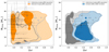 |
Fig. 1. Joint distribution of the chirp mass, Mchirp, and the effective inspiral spin parameter, χeff, for the combined CE, SMT, and CHE channels. For both sub-figures, the model predictions for the underlying (intrinsic) BBH population are shown in gray, where lighter shades represent larger contour levels of 90% and 99.9%, respectively. Left: detected BBH population with O3 sensitivity, shown in orange. Overlaid in black are the O1, O2, and O3a of the LIGO Scientific and Virgo Collaboration (LVC) GWTC-2 (Abbott et al. 2021a) data with their 90% CIs; GW190521 is outside the plotted window. Right: BBH subpopulation that emitted LGRBs at BBH formation, shown in blue. The ten events in GWTC-2 with chances > 10% of having emitted a luminous LGRB at BBH formation are indicated in black. The two events with > 50% probabilities, GW190517 and GW190719, are indicated with star markers. No bin smoothing was applied when constructing the contour levels. |
Contemporary GW detectors can probe only the low-redshift subset (z ≲ 1, Abbott et al. 2021b) of the underlying BBH population. Observations are biased toward high Mchirp as the signals of massive BBHs are louder and, hence, can be detected at further distances. Current GW observatories are therefore unable to individually resolve a large fraction of merging BBHs in the Universe. In the left panel of Fig. 1, we indicate the observed distribution of χeff and Mchirp predicted by our model, assuming a three-detector configuration with a network signal-to-noise ratio threshold of 12 and “mid-high–late-low” sensitivity (Abbott et al. 2018), consistent with the third observing run of the LIGO and Virgo detectors. For a direct comparison with the observations, we overlay the 46 BBH events with their 90% credible interval (CI). The GW detector selection effects distort the observable distributions to high Mchirp and χeff values compared to the underlying BBH distribution.
A fraction of the underlying merging BBH population with fast-spinning BHs is expected to give rise to LGRB events at the moment of BBH formation. For each BBH formation, we calculated from the structure profile of the BH progenitor star whether a sufficiently massive accretion disk is formed during the core collapse, which would give rise to a luminous LGRB (see Appendix C for details). In the CE channel, only the second-born BH is associated with an LGRB as tidal interactions are only relevant in the BH–Wolf-Rayet evolution phase of the BBH progenitor. In contrast, a fast-spinning CHE BBH system can be associated with two LGRB events, as tides cause both stars to be rapidly spinning. The subpopulation of BBHs associated with LGRBs shown in the right panel of Fig. 1. These systems have χeff ≳ 0.2 (90% CI) while favoring Mchirp ∈ [5, 30] M⊙. In contrast to the observed GW population, there is no observational bias for high-Mchirp BHs in the LGRB population. We find that the expected number of GWTC-2 events that had emitted an LGRB at BBH formation is ≈4. Among all the GWTC-2 events, GW190517 and GW190719 have the highest probabilities, ≈85% and ≈60% respectively, of having had an LGRB precursor, while eight more events have a probability pLGRB > 10%. Those ten events are highlighted in the right panel of Fig. 1. The details of the calculation of these probabilities are presented in Appendix E.
The combined local (z = 0) BBH merger rate density of our CE, SMT, and CHE fiducial models is 38.3 Gpc−3 yr−1, with each channel contributing 57%, 29%, and 14%, respectively. The predicted local rate density is within the observational constraints from GWTC-2 with [15.3, 38.8] Gpc−3 yr−1 at 90% credibility (Abbott et al. 2021a). In Fig. 2, we show the redshift evolution of each channel’s BBH merger rate density as well as their combination. The CE BBH merger rate density peaks at a redshift z ∈ [2, 3], close to the peak of the SFR density. The CE BBH merger rate closely follows the SFR because of the short delay times between the formation and merger of tight BBH systems produced by the CE channel. In contrast, SMT and CHE BBHs have longer delay timescales as there is no mechanism to shrink the orbits as efficiently as the CE phase does. Therefore, the SMT rate density does not follow the SFR density and peaks at lower redshifts. Finally, we note that the CHE rate density is not as suppressed at high redshifts as in the other two channels. This is because the CHE channel operates with higher efficiency at extremely low metallicity environments, which are more abundant at high redshifts.
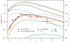 |
Fig. 2. Modeled merging BBH and luminous LGRB rate densities as a function of redshift from isolated binary evolution in dashed and solid black lines, respectively. The CE, SMT, and CHE channel contributions are indicated in orange, blue, and green colors, respectively. The violet marker denotes observable constraints of local BBH rate densities at z = 0 from LVC GWTC-2 (Abbott et al. 2021a) and the red markers the luminous LGRB rate densities from the SHOALS survey (Perley et al. 2016). The SHOALS survey LGRB rate densities are not beaming-corrected and hence probe the observed and not the intrinsic LGRB population. Our fiducial model assumes LGRB efficiency η = 0.01, constant beaming factor fB = 0.05, and IllustrisTNG redshift- and metallicity-dependent star formation rate (Nelson et al. 2019). |
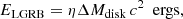
Luminous LGRB rate densities from our fiducial model are shown in Fig. 2 as a function of redshift, for each channel and their combination (solid lines). The fiducial model assumes an LGRB energy efficiency η = 0.01 and beaming fraction fB = 0.05, whose ratio is calibrated to match the peak of observed luminous LGRB energy distributions as described in Appendix C and shown in Fig. 3. The majority of LGRBs originate through the CE evolutionary pathway while only 21–25%, for any z < 10, come from CHE. The SMT channel leads to the smallest LGRB rate densities (< 0.03 Gpc−3 yr−1) for any redshift, as tidally spun-up second-born BHs are rare in this evolutionary pathway. To test our model predictions, we compare our theoretical luminous LGRB rate estimates with the SHOALS survey estimates in Fig. 2. The combination of CE and CHE LGRB rates for our fiducial model are consistent with the observations of luminous LGRBs throughout the redshift range. A discussion on the sensitivity of our rate estimates regarding the choice of beaming fractions and SFR is presented in Appendices C and D.
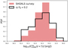 |
Fig. 3. Normalized histogram of the observed luminous LGRB isotropic-equivalent energies with redshift z < 5 from the SHOALS survey, in light red, compared to the modeled LGRB isotropic-equivalent energies. Our fiducial model was calibrated such that the modeled LGRB energies peak near the observed energy distribution. This is achieved for |
Long-duration gamma-ray bursts probe the formation of fast-spinning merging BBHs formed at low metallicity because, at such metallicities, stellar winds are weaker, which allows the BBHs’ progenitors to remain rapidly spinning and in close orbits until the formation of the BHs. These systems are therefore mostly formed at high redshifts where low metallicity environments are more abundant. Measurements of the metallicity of LGRB host galaxies have shown that LGRB rates are indeed enhanced at low metallicities (Fruchter et al. 2006). In our model, the threshold for LGRB formation is Zmax ≈ 0.2 Z⊙ where we adopt Z⊙ = 0.017 (Grevesse et al. 1996). In Fig. 4, we compare the progenitors’ metallicities of modeled LGRBs to the subsample of the SHOALS LGRBs with identified host galaxies that have measured metallicities for z < 2.5 (Graham et al. 2019). At face value, we find that 40% of the observed LGRB host galaxies have metallicities lower than Zmax. However, when taking possible systematic uncertainties in the measurement of log10(O/H) abundances into account (Kewley & Ellison 2008) our model can be consistent with at most ∼85% of observed LGRBs (see Appendix F for more details). Selection effects in LGRB host galaxies for which metallicity measurements are possible bias the sample toward low redshift and high-mass galaxies, and hence potentially toward higher metallicities (Graham et al. 2019). This comparison implies that in order to associate the entirety of luminous LGRBs with the formation of BBHs, a potentially significant fraction of LGRB progenitors at low redshifts (z < 2.5) must originate in low metallicity pockets of the host galaxies. Finally, we should stress that theoretical model uncertainties due to the uncertain metallicity dependence of stellar wind mass loss during the late Wolf-Rayet phase of the stars evolution as well as the uncertainties in the metallicity-dependent SFR make this comparison less conclusive. A detailed parameter study would improve such a comparison but is beyond the scope of this Letter.
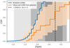 |
Fig. 4. Cumulative distribution function (CDF) of the modeled LGRB progenitors’ metallicities for redshifts z < 2.5, in blue. The CDF of the observed SHOALS LGRB host galaxy metallicities for z < 2.5 (Graham et al. 2019) are indicated in orange. The light orange shaded area shows the uncertainty in the observed CDF due to systematic offsets in the measurement of log10(O/H), depending on the calibrations used, and the stellar mass of the galaxy which can be as high as Δ[log10(O/H)] ≈ 0.7 dex (Kewley & Ellison 2008). As a reference, we indicate with a vertical dashed black line the median metallicity from the IllustrisTNG simulation at redshift z = 2, and lighter gray shaded areas delineate larger CIs of 68%, 95%, and 99% for the assumed star formation metallicity distribution. |
4. Discussion and conclusions
In this study we only consider a contribution to the LGRB rate from merging BBH progenitors. Other pathways to fast-spinning BH progenitor stars, in single or binary systems, have been proposed to lead to LGRBs (e.g., Yoon et al. 2006; Cantiello et al. 2007), albeit none at a rate that matches the observed one when considering efficient AM transport in stellar interiors (Fryer et al. 2007). Observed high-mass X-ray binaries that contain fast-spinning BHs, such as Cygnus X-1 (e.g., Gou et al. 2011; Zhao et al. 2021), may have also been progenitors of LGRBs. The formation of these systems is puzzling (e.g., Wong et al. 2012; Neijssel et al. 2021), and it is uncertain whether the BH spin in these systems originates from fast-spinning pre-collapse cores (see, e.g., Moreno Méndez et al. 2008; Batta et al. 2017; Schrøder et al. 2018). It is interesting to note that a simple estimate of the LGRB rate density from Cyg X-1-like systems, assuming that there is one such binary per Milky Way-like galaxy with SFRMW ≃ 1 M⊙ yr−1 and assuming a typical lifetime of τHMXB ≃ 105 yr, far exceeds the observationally determined one at ℛLGRB(z ≃ 0) < 0.6 Gpc−3 yr−1 of
In this estimate, we assumed an SFR(z ≃ 0) = 2 × 10⁷ M⊙ Gpc−3 yr−1 for the local Universe (cf. Fig. 1). Another viable alternative for the origin of LGRBs includes the formation of a fast-rotating neutron star (NS) with an ultrahigh magnetic field (Duncan & Thompson 1992). While our analysis cannot exclude other potential progenitors of LGRBs, consideration of the salient uncertainties of our model demonstrates that progenitors of fast-spinning BBH mergers, formed via isolated binary evolution, are likely a major contribution to the observed luminous LGRB rate.
Fast-spinning BBHs typically have short merger timescales. Because of this, current GW detectors cannot probe them efficiently, as their formation and merger rate is maximal approximately where the SFR density peaks at z ∈ [2, 3]. Luminous LGRBs, on the other hand, are observable up to a redshift of ≈9 and can therefore be used as a cosmological probe, empirically constraining the subpopulation of progenitors of fast-spinning BBH merger events far beyond the horizons of current-generation GW observatories. We used two types of multi-messenger, albeit asynchronous, observations – GWs and gamma-rays – to chart BBH formation across cosmic time. Using combinations of observations in this way opens a new avenue to constraining the currently uncertain physics of binary evolution and compact object formation.
Acknowledgments
We would like to thank Christopher Berry for his comments on the manuscript. This work was supported by the Swiss National Science Foundation Professorship grant (project number PP00P2_176868). E. R.-R. acknowledges support from the Heising-Simons Foundation, the Danish National Research Foundation (DNRF132) and NSF (AST-1911206 and AST-1852393). P. M. is supported by the FWO junior postdoctoral fellowship No. 12ZY520N. L. Z. K. is supported by CIERA. M. Z. is supported by NASA through the NASA Hubble Fellowship grant HST-HF2-51474.001-A awarded by the Space Telescope Science Institute, which is operated by the Association of Universities for Research in Astronomy, Inc., for NASA, under contract NAS5-26555. J. J. A. and S. C. are supported by CIERA and A. D., J. G. S. P., and K. A. R. are supported by the Gordon and Betty Moore Foundation through grant GBMF8477. Y. Q. acknowledges funding from the Swiss National Science Foundation under grant P2GEP2_188242. The computations were performed in part at the University of Geneva on the Baobab and Yggdrasil computer clusters and at Northwestern University on the Trident computer cluster (the latter funded by the GBMF8477 grant). All figures were made with the open-source Python modules Corner (Foreman-Mackey 2016) and Matplotlib (Hunter 2007). This research made use of the python modules (Virtanen et al. 2020), Astropy (Astropy Collaboration 2018), and PyCBC (Nitz et al. 2019).
References
- Aasi, J., Abbott, B. P., Abbott, R., et al. 2015, CQG, 32, 074001 [Google Scholar]
- Abbott, B. P., Abbott, R., Abbott, T. D., et al. 2018, Liv. Rev. Rel., 21, 3 [Google Scholar]
- Abbott, R., Abbott, T. D., Abraham, S., et al. 2021a, Phys. Rev. X, 11, 021053 [Google Scholar]
- Abbott, R., Abbott, T. D., Abraham, S., et al. 2021b, ApJ, 913, L7 [NASA ADS] [CrossRef] [Google Scholar]
- Acernese, F., Agathos, M., Agatsuma, K., et al. 2015, CQG, 32, 024001 [NASA ADS] [CrossRef] [Google Scholar]
- Antonini, F., Gieles, M., & Gualandris, A. 2019, MNRAS, 486, 5008 [NASA ADS] [CrossRef] [Google Scholar]
- Astropy Collaboration (Price-Whelan, A. M., et al.) 2018, AJ, 156, 123 [Google Scholar]
- Bardeen, J. M. 1970, Nature, 226, 64 [Google Scholar]
- Batta, A., & Ramirez-Ruiz, E. 2019, ArXiv e-prints [arXiv:1904.04835] [Google Scholar]
- Batta, A., Ramirez-Ruiz, E., & Fryer, C. 2017, ApJ, 846, L15 [NASA ADS] [CrossRef] [Google Scholar]
- Bavera, S. S., Fragos, T., Qin, Y., et al. 2020, A&A, 635, A97 [NASA ADS] [CrossRef] [EDP Sciences] [Google Scholar]
- Bavera, S. S., Fragos, T., Zevin, M., et al. 2021a, A&A, 647, A153 [NASA ADS] [CrossRef] [EDP Sciences] [Google Scholar]
- Bavera, S. S., Zevin, M., & Fragos, T. 2021b, Res. Notes Am. Astron. Soc., 5, 127 [Google Scholar]
- Bavera, S. S., Franciolini, G., Cusin, G., et al. 2022, A&A, in press, https://doi.org/10.1051/0004-6361/202142208 [NASA ADS] [CrossRef] [EDP Sciences] [Google Scholar]
- Belczynski, K., Holz, D. E., Bulik, T., & O’Shaughnessy, R. 2016, Nature, 534, 512 [NASA ADS] [CrossRef] [Google Scholar]
- Belczynski, K., Klencki, J., Fields, C. E., et al. 2020, A&A, 636, A104 [NASA ADS] [CrossRef] [EDP Sciences] [Google Scholar]
- Berger, L., Koester, D., Napiwotzki, R., Reid, I. N., & Zuckerman, B. 2005, A&A, 444, 565 [NASA ADS] [CrossRef] [EDP Sciences] [Google Scholar]
- Breivik, K., Coughlin, S., Zevin, M., et al. 2020, ApJ, 898, 71 [Google Scholar]
- Cantiello, M., Yoon, S. C., Langer, N., & Livio, M. 2007, A&A, 465, L29 [NASA ADS] [CrossRef] [EDP Sciences] [Google Scholar]
- Chrimes, A. A., Stanway, E. R., & Eldridge, J. J. 2020, MNRAS, 491, 3479 [NASA ADS] [CrossRef] [Google Scholar]
- Claeys, J. S. W., Pols, O. R., Izzard, R. G., Vink, J., & Verbunt, F. W. M. 2014, A&A, 563, A83 [NASA ADS] [CrossRef] [EDP Sciences] [Google Scholar]
- Cucchiara, A., Levan, A. J., Fox, D. B., et al. 2011, ApJ, 736, 7 [Google Scholar]
- Deheuvels, S., Ballot, J., Beck, P. G., et al. 2015, A&A, 580, A96 [NASA ADS] [CrossRef] [EDP Sciences] [Google Scholar]
- De Luca, V., Franciolini, G., Pani, P., & Riotto, A. 2020, JCAP, 2020, 044 [Google Scholar]
- de Mink, S. E., Cantiello, M., Langer, N., et al. 2009, A&A, 497, 243 [NASA ADS] [CrossRef] [EDP Sciences] [Google Scholar]
- Detmers, R. G., Langer, N., Podsiadlowski, P., & Izzard, R. G. 2008, A&A, 484, 831 [NASA ADS] [CrossRef] [EDP Sciences] [Google Scholar]
- du Buisson, L., Marchant, P., Podsiadlowski, P., et al. 2020, MNRAS, 499, 5941 [Google Scholar]
- Duncan, R. C., & Thompson, C. 1992, ApJ, 392, L9 [Google Scholar]
- Eggleton, P. P. 1983, ApJ, 268, 368 [Google Scholar]
- Foreman-Mackey, D. 2016, J. Open Source Software, 1, 24 [NASA ADS] [CrossRef] [Google Scholar]
- Fragos, T., & McClintock, J. E. 2015, ApJ, 800, 17 [Google Scholar]
- Fragos, T., Andrews, J. J., Ramirez-Ruiz, E., et al. 2019, ApJ, 883, L45 [Google Scholar]
- Frail, D. A., Kulkarni, S. R., Sari, R., et al. 2001, ApJ, 562, L55 [NASA ADS] [CrossRef] [Google Scholar]
- Franciolini, G., Baibhav, V., De Luca, V., et al. 2021, ArXiv e-prints [arXiv:2105.03349] [Google Scholar]
- Fruchter, A. S., Levan, A. J., Strolger, L., et al. 2006, Nature, 441, 463 [NASA ADS] [CrossRef] [Google Scholar]
- Fryer, C. L., Mazzali, P. A., Prochaska, J., et al. 2007, PASP, 119, 1211 [NASA ADS] [CrossRef] [Google Scholar]
- Fryer, C. L., Belczynski, K., Wiktorowicz, G., et al. 2012, ApJ, 749, 91 [Google Scholar]
- Fuller, J., & Ma, L. 2019, ApJ, 881, L1 [Google Scholar]
- Fuller, J., Piro, A. L., & Jermyn, A. S. 2019, MNRAS, 485, 3661 [NASA ADS] [Google Scholar]
- Gehan, C., Mosser, B., Michel, E., Samadi, R., & Kallinger, T. 2018, A&A, 616, A24 [NASA ADS] [CrossRef] [EDP Sciences] [Google Scholar]
- Goldstein, A., Connaughton, V., Briggs, M. S., & Burns, E. 2016, ApJ, 818, 18 [CrossRef] [Google Scholar]
- Gou, L., McClintock, J. E., Reid, M. J., et al. 2011, ApJ, 742, 85 [NASA ADS] [CrossRef] [Google Scholar]
- Graham, J. F., Schady, P., & Fruchter, A. S. 2019, ArXiv e-prints [arXiv:1904.02673] [Google Scholar]
- Grevesse, N., & Sauval, A. J. 1998, Space Sci. Rev., 85, 161 [Google Scholar]
- Grevesse, N., Noels, A., & Sauval, A. J. 1996, in Cosmic Abundances, eds. S. S. Holt, & G. Sonneborn, ASP Conf. Ser., 99, 117 [Google Scholar]
- Heger, A., Woosley, S., Baraffe, I., & Abel, T. 2002, in Lighthouses of the Universe: The Most Luminous Celestial Objects and Their Use for Cosmology, eds. M. Gilfanov, R. Sunyeav, & E. Churazov, 369 [Google Scholar]
- Hobbs, G., Lorimer, D. R., Lyne, A. G., & Kramer, M. 2005, MNRAS, 360, 974 [Google Scholar]
- Hunter, J. D. 2007, Comput. Sci. Eng., 9, 90 [NASA ADS] [CrossRef] [Google Scholar]
- Inayoshi, K., Hirai, R., Kinugawa, T., & Hotokezaka, K. 2017, MNRAS, 468, 5020 [Google Scholar]
- Ivanova, N., Justham, S., Chen, X., et al. 2013, A&ARv, 21, 59 [Google Scholar]
- Kalogera, V. 1996, ApJ, 471, 352 [Google Scholar]
- Kalogera, V., Belczynski, K., Kim, C., O’Shaughnessy, R., & Willems, B. 2007, Phys. Rep., 442, 75 [Google Scholar]
- Kewley, L. J., & Ellison, S. L. 2008, ApJ, 681, 1183 [Google Scholar]
- Klencki, J., Nelemans, G., Istrate, A. G., & Chruslinska, M. 2021, A&A, 645, A54 [EDP Sciences] [Google Scholar]
- Kobulnicky, H. A., & Kewley, L. J. 2004, ApJ, 617, 240 [CrossRef] [Google Scholar]
- Kouveliotou, C., Meegan, C. A., Fishman, G. J., et al. 1993, ApJ, 413, L101 [NASA ADS] [CrossRef] [Google Scholar]
- Kroupa, P. 2001, MNRAS, 322, 231 [NASA ADS] [CrossRef] [Google Scholar]
- Kurtz, D. W., Saio, H., Takata, M., et al. 2014, MNRAS, 444, 102 [Google Scholar]
- Madau, P., & Fragos, T. 2017, ApJ, 840, 39 [Google Scholar]
- Mandel, I., & de Mink, S. E. 2016, MNRAS, 458, 2634 [NASA ADS] [CrossRef] [Google Scholar]
- Marchant, P., Langer, N., Podsiadlowski, P., Tauris, T. M., & Moriya, T. J. 2016, A&A, 588, A50 [NASA ADS] [CrossRef] [EDP Sciences] [Google Scholar]
- Marchant, P., Renzo, M., Farmer, R., et al. 2019, ApJ, 882, 36 [Google Scholar]
- Marchant, P., Pappas, K. M. W., Gallegos-Garcia, M., et al. 2021, A&A, 650, A107 [NASA ADS] [CrossRef] [EDP Sciences] [Google Scholar]
- Modjaz, M., Liu, Y. Q., Bianco, F. B., & Graur, O. 2016, ApJ, 832, 108 [NASA ADS] [CrossRef] [Google Scholar]
- Moe, M., & Di Stefano, R. 2017, ApJS, 230, 15 [Google Scholar]
- Moreno Méndez, E., Brown, G. E., Lee, C.-H., & Park, I. H. 2008, ApJ, 689, L9 [CrossRef] [Google Scholar]
- Neijssel, C. J., Vigna-Gómez, A., Stevenson, S., et al. 2019, MNRAS, 490, 3740 [Google Scholar]
- Neijssel, C. J., Vinciguerra, S., Vigna-Gómez, A., et al. 2021, ApJ, 908, 118 [NASA ADS] [CrossRef] [Google Scholar]
- Nelson, D., Springel, V., Pillepich, A., et al. 2019, Comput. Astrophys. Cosmol., 6, 2 [Google Scholar]
- Nicholls, D. C., Sutherland, R. S., Dopita, M. A., Kewley, L. J., & Groves, B. A. 2017, MNRAS, 466, 4403 [Google Scholar]
- Nitz, A., Harry, I., Brown, D., et al. 2019, gwastro/pycbc: PyCBC Release v1.14.4 [Google Scholar]
- Nugis, T., & Lamers, H. J. G. L. M. 2000, A&A, 360, 227 [NASA ADS] [Google Scholar]
- Paczyński, B. 1998, ApJ, 494, L45 [Google Scholar]
- Patton, R. A., & Sukhbold, T. 2020, MNRAS, 499, 2803 [NASA ADS] [CrossRef] [Google Scholar]
- Paxton, B., Bildsten, L., Dotter, A., et al. 2011, ApJS, 192, 3 [Google Scholar]
- Paxton, B., Cantiello, M., Arras, P., et al. 2013, ApJS, 208, 4 [Google Scholar]
- Paxton, B., Marchant, P., Schwab, J., et al. 2015, ApJS, 220, 15 [Google Scholar]
- Paxton, B., Schwab, J., Bauer, E. B., et al. 2018, ApJS, 234, 34 [NASA ADS] [CrossRef] [Google Scholar]
- Paxton, B., Smolec, R., Schwab, J., et al. 2019, ApJS, 243, 10 [Google Scholar]
- Pejcha, O., & Thompson, T. A. 2015, ApJ, 801, 90 [NASA ADS] [CrossRef] [Google Scholar]
- Perley, D. A., Krühler, T., Schulze, S., et al. 2016, ApJ, 817, 7 [Google Scholar]
- Planck Collaboration XIII. 2016, A&A, 594, A13 [NASA ADS] [CrossRef] [EDP Sciences] [Google Scholar]
- Postnov, K. A., & Yungelson, L. R. 2014, Liv. Rev. Rel., 17, 3 [NASA ADS] [CrossRef] [Google Scholar]
- Qin, Y., Fragos, T., Meynet, G., et al. 2018, A&A, 616, A28 [NASA ADS] [CrossRef] [EDP Sciences] [Google Scholar]
- Quast, M., Langer, N., & Tauris, T. M. 2019, A&A, 628, A19 [NASA ADS] [CrossRef] [EDP Sciences] [Google Scholar]
- Rodriguez, C. L., Zevin, M., Amaro-Seoane, P., et al. 2019, Phys. Rev. D, 100, 043027 [Google Scholar]
- Román-Garza, J., Bavera, S. S., Fragos, T., et al. 2021, ApJ, 912, L23 [CrossRef] [Google Scholar]
- Sana, H., de Mink, S. E., de Koter, A., et al. 2012, Science, 337, 444 [Google Scholar]
- Sari, R., Piran, T., & Halpern, J. P. 1999, ApJ, 519, L17 [CrossRef] [Google Scholar]
- Sasaki, M., Suyama, T., Tanaka, T., & Yokoyama, S. 2016, Phys. Rev. Lett., 117, 061101 [NASA ADS] [CrossRef] [Google Scholar]
- Schneider, F. R. N., Podsiadlowski, P., & Müller, B. 2021, A&A, 645, A5 [NASA ADS] [CrossRef] [EDP Sciences] [Google Scholar]
- Schrøder, S. L., Batta, A., & Ramirez-Ruiz, E. 2018, ApJ, 862, L3 [CrossRef] [Google Scholar]
- Smarr, L. L., & Blandford, R. 1976, ApJ, 207, 574 [Google Scholar]
- Spruit, H. C. 1999, A&A, 349, 189 [NASA ADS] [Google Scholar]
- Spruit, H. C. 2002, A&A, 381, 923 [CrossRef] [EDP Sciences] [Google Scholar]
- Sukhbold, T., Ertl, T., Woosley, S. E., Brown, J. M., & Janka, H. T. 2016, ApJ, 821, 38 [NASA ADS] [CrossRef] [Google Scholar]
- Taylor, P. A., Miller, J. C., & Podsiadlowski, P. 2011, MNRAS, 410, 2385 [CrossRef] [Google Scholar]
- Thorne, K. S. 1974, ApJ, 191, 507 [Google Scholar]
- Tout, C. A., Pols, O. R., Eggleton, P. P., & Han, Z. 1996, MNRAS, 281, 257 [Google Scholar]
- Tutukov, A. V., & Yungelson, L. R. 1993, MNRAS, 260, 675 [Google Scholar]
- van den Heuvel, E. P. J. 1976, in Structure and Evolution of Close Binary Systems, eds. P. Eggleton, S. Mitton, & J. Whelan, 73, 35 [Google Scholar]
- van den Heuvel, E. P. J., & Yoon, S. C. 2007, Ap&SS, 311, 177 [NASA ADS] [CrossRef] [Google Scholar]
- van den Heuvel, E. P. J., Portegies Zwart, S. F., & de Mink, S. E. 2017, MNRAS, 471, 4256 [Google Scholar]
- Vink, J. S., de Koter, A., & Lamers, H. J. G. L. M. 2001, A&A, 369, 574 [NASA ADS] [CrossRef] [EDP Sciences] [Google Scholar]
- Virtanen, P., Gommers, R., Oliphant, T. E., et al. 2020, Nat. Methods, 17, 261 [Google Scholar]
- Wong, T.-W., Valsecchi, F., Fragos, T., & Kalogera, V. 2012, ApJ, 747, 111 [NASA ADS] [CrossRef] [Google Scholar]
- Woosley, S. E. 1993, ApJ, 405, 273 [Google Scholar]
- Woosley, S. E., & Bloom, J. S. 2006, ARA&A, 44, 507 [Google Scholar]
- Yoon, S. C., Langer, N., & Norman, C. 2006, A&A, 460, 199 [NASA ADS] [CrossRef] [EDP Sciences] [Google Scholar]
- Zevin, M., Spera, M., Berry, C. P. L., & Kalogera, V. 2020, ApJ, 899, L1 [Google Scholar]
- Zevin, M., Bavera, S. S., Berry, C. P. L., et al. 2021, ApJ, 910, 152 [Google Scholar]
- Zhao, X., Gou, L., Dong, Y., et al. 2021, ApJ, 908, 117 [NASA ADS] [CrossRef] [Google Scholar]
Appendix A: Population synthesis of CE, SMT, and CHE binary black holes
We modeled the evolution of binaries through CE and SMT with the POSYDON framework to combine the rapid population synthesis code COSMIC (Breivik et al. 2020) with detailed MESA (Paxton et al. 2011, 2013, 2015, 2018, 2019) stellar structure and binary evolution simulations (Bavera et al. 2022). This hybrid approach is used to rapidly evolve millions of binaries from the zero-age main sequence (ZAMS) until the end of the second MT episode. For the last phase of the evolution, which determines the second-born BH spin (Qin et al. 2018; Bavera et al. 2020), we used detailed BH–Wolf-Rayet binary evolution simulations to model the tidal spin-up phase until the secondary star reaches central carbon exhaustion. These simulations take differential stellar rotation, tides, stellar winds, and the evolution of the Wolf–Rayet stellar structure until carbon depletion into account. The core collapse was modeled as described in the next section. We consider disk formation during the collapse of fast-spinning stars, mass loss through neutrinos, pulsational pair-instability supernovae (PPISNe) and pair-instability supernovae (PISNe; Marchant et al. 2019), and orbital changes resulting from anisotropic mass loss and isotropic neutrino mass loss (Kalogera 1996).
In our models the first-born BHs in the SMT and CE channels are formed with a negligible spin because of the assumed efficient AM transport (Fragos & McClintock 2015; Qin et al. 2018; Fuller & Ma 2019). If AM transport were to be inefficient, this would lead to spinning BBHs (Belczynski et al. 2020), which is currently inconsistent with GWTC-2 observations. Moreover, we assumed Eddington-limited accretion efficiency onto compact objects, resulting in a negligible amount of mass accreted onto the first-born BH during SMT. Hence, the first-born BH in the SMT channel avoids any spin-up during MT (Thorne 1974). Alternatively, if the accretion onto compact objects reached highly super-Eddington rates, the binaries would not shrink enough to produce merging BBHs, leading to the suppression of the SMT channel (Bavera et al. 2022). Hence, even though super-Eddington accretion efficiency strongly affects the yield of merging BBHs through the SMT channel, it will not affect LGRBs rates as the MT accretion spin-up occurs after BH formation. Finally, motivated by the model comparison between our models and GWTC-2 data (Bavera et al. 2022), we assumed low CE ejection efficiencies, taken as αCE = 0.5 in the αCE − λ CE parameterization theory (see, e.g., Ivanova et al. 2013, for a review) and adopted λ fits as in Claeys et al. (2014). Because the post-CE orbital separation is approximately proportional to αCE, inefficient CE ejection leads, on average, to a larger fraction of tidally spun-up BHs and, at the same time, to a smaller overall number of BBH merger events compared to efficient CE ejection, αCE > 1. Here, an αCE value greater than 1 does not necessarily mean that other sources of energy partake in the CE ejection; it more likely points to an inaccurate assumption of core-envelope boundaries. Indeed, multiple recent studies (Fragos et al. 2019; Quast et al. 2019; Klencki et al. 2021; Marchant et al. 2021) have shown that envelope stripping stops earlier than what is currently assumed in population synthesis. We find that this model’s uncertainty changes our LGRB rate estimate by  at redshift z = 0 (z = 2) by +36% (+18%), −56% (−42%) and −68% (−54%) for αCE = 0.25, 1, and 2, respectively; this does not change the conclusion of our study.
The binary evolution through CHE is modeled entirely with MESA until the carbon depletion of both stars (du Buisson et al. 2020). More precisely, we modeled the two stars simultaneously in a binary system where tidal interaction and MT are taken into account. For consistency, the CE and SMT MESA models used input physics identical to the CHE ones, and simulations with the COSMIC code were also configured to be as consistent as possible (Bavera et al. 2022; Zevin et al. 2021). Similar to the other channels, the core collapse of stars’ profiles’ was done self-consistently with CE and SMT models using POSYDON. Because the CHE MESA grids assume a fixed mass ratio of q = 1, both stars will reach core collapse simultaneously. In practice, we collapsed one star after the other by applying a Blauw kick (Kalogera 1996) after each star has collapsed to account for the orbit adjustment resulting from PPISN and neutrino mass loss, where we assume circularization after the formation of the first BH (du Buisson et al. 2020).
Initial binary conditions at ZAMS were drawn randomly from empirically constrained distributions. In CE and SMT, the ZAMS binaries were directly evolved with POSYDON while binaries in the parameter space leading to CHE were mapped to the nearest neighbor CHE MESA evolutionary track. Metallicities were sampled in the log-range log10(Z)∈[−5, log10(2 Z⊙)]. For the CE and SMT models the log-metallicity range was divided into 30 discrete values from log10(Z) = − 4 to log10(1.5 Z⊙), where binaries with log10(Z)∈[−5, −4] were mapped to the lowest metallicity bin (Bavera et al. 2022). For the CHE models the log-metallicity range was sampled with 22 discrete values from log10(Z) = − 5.0 to log10(Z) = − 2.375, above which any binary evolves through the CHE channel (du Buisson et al. 2020). Primary masses follow the Kroupa initial mass function (IMF), a broken power law with coefficient α = −2.3 (Kroupa 2001) in the sampled mass range 5 M⊙ ≤ m1 ≤ 150 M⊙. The upper limit is an extrapolation of the original Kroupa IMF measured only up to 50 M⊙. The arbitrary maximum stellar mass was chosen to exclude BH formation above the upper mass gap of PISNe, which we did not model (Heger et al. 2002). The mass distribution of the less massive secondary star is given by m2 = m1 × q, where the initial mass ratio q is drawn from a flat distribution (Sana et al. 2012) in the range q ∈ (0, 1]. We assumed that all binaries are born with circular orbits. Furthermore, we adopted a binary fraction of fbin = 0.7 (Sana et al. 2012) and assume that at birth the distribution of log-orbital periods follows a power law with coefficient π = −0.55 (Sana et al. 2012) in the range log10(p/[day]) ∈ [0.15, 5.5] and extrapolated down to the range log10(p/[day]) ∈ [log10(0.4/[day]), 0.15] assuming a log-flat distribution (Bavera et al. 2022). The portion of the parameter space with q ∈ [0.8, 1] and p ∈ [0.4, 4] days may lead to CHE (du Buisson et al. 2020). It should be noticed that there are some uncertainties on the actual initial binary properties of mass ratios, periods, and eccentricities (see, e.g., Moe & Di Stefano 2017), however, there are no constraints on these properties at low metallicities, such as the metallicities modeled here. Moreover, the extrapolation to low orbital periods led us to sample the systems’ Roche-lobe overflow at ZAMS. Therefore, these systems underwent MT during the pre-main-sequence phase, which complicates the binary evolution and, a priori, might not lead to CHE. To remove these systems from the sampled distribution, we adopted ZAMS stellar radii fits (Tout et al. 1996), which we compare to the initial Roche-lobe radii of the binary (Eggleton 1983). The population synthesis will then result in a synthetic population of BBHs, which we distributed across the cosmic history of the Universe to compute rate densities (see Appendix B for a detailed description).
Appendix B: LGRB collapsar scenario
A massive star collapses under its own weight when nuclear reactions can no longer generate enough pressure to balance the pull of gravity. For the most massive stars, this occurs after the stars have formed iron cores. Due to computational constraints, our MESA simulations run until carbon depletion, which occurs less than a year before the actual core collapse. Because the remaining stellar evolutionary phase is so rapid compared to the star’s total evolution, we can assume that the star’s structure will not change drastically in the neglected portion of the evolution. The core collapse was modeled using fits to the results of 2D core-collapse models (Fryer et al. 2012). We also accounted for mass loss through PPISNe or stellar disruption from PISNe using fits to 1D stellar models that target this evolution phase (Marchant et al. 2019). Depending on the carbon-oxygen core mass, mCO − core, the star might explode as a supernova and have a fraction of the ejected mass fall back onto the compact object, or, if the star is massive enough, where mCO − core ≥ 11 M⊙, the star will collapse directly to form a BH (Fryer et al. 2012). Consequently, in our models only stars with mCO − core ≤ 11 M⊙ can receive natal kicks, with magnitudes drawn from a Maxwellian distribution with σ = 265 km/s (Hobbs et al. 2005) and rescaled by one minus the fall-back mass fraction (Fryer et al. 2012). In this case, only a negligible fraction of such low-mass, merging, fast-spinning BBHs associated with LGRBs will be disrupted by natal kicks as they are in tight orbits (orbital periods of less than one day), and hence, only a kick with a magnitude larger than the corresponding orbital velocity, vorb > 500 km/s, can disrupt the system. Furthermore, we notice that newer studies on core-collapse physics (e.g., Pejcha & Thompson 2015; Sukhbold et al. 2016; Patton & Sukhbold 2020; Schneider et al. 2021) indicate that there is no such distinct monotonic relation between NS and BH formation (for a detailed study of the impact of newer core-collapse mechanism prescriptions on the formation of merging BBH and BH-NS in our models, see Román-Garza et al. (2021)). In the collapse, we also account for up to 0.5 M⊙ of mass loss through neutrinos (Zevin et al. 2020). If the collapsing star is rapidly rotating, an accretion disk might form during this process (Bavera et al. 2022). Because our MESA simulations provide us with the star’s profile at core collapse, we can estimate the amount of material that forms an accretion disk around the newly formed BH as well as the spin of the final BH (Batta & Ramirez-Ruiz 2019). We assumed that the innermost shells of the star form a central BH of mass 2.5 M⊙ through direct collapse, where we account for the mass and AM loss through neutrinos (Bavera et al. 2022). The collapse of each subsequent shell happens on a dynamical timescale. We accounted for each shell’s portion with enough specific AM to support disk formation instead of collapsing directly. The thin disk is subsequently accreted on a viscous timescale which we assumed to be much smaller than the dynamical timescale. Hence the disk is accreted before the next shell collapses. We notice that the accretion problem might be more complex than what has been assumed; for example Taylor et al. (2011) 3D smoothed-particle hydrodynamics simulations showed that hydrodynamical instabilities in the accretion disk may result in intermittent accretion. If this is the case one would also need to account for feedback from the already-accreted disk to the rest of the in-falling material (see, e.g., Bavera et al. 2021b) which we do not do here. When an accretion disk is formed, a fraction of its rest-mass energy can power the formation of a jet that pierces through the star and breaks out from its poles. This mechanism is known as the collapsar scenario and is thought to give rise to LGRBs (Woosley 1993; Paczyński 1998).
Appendix C: LGRB isotropic-equivalent energy calibration
The LGRB jet is powered by the accretion disk produced in the core-collapse, and only a fraction, fjet, of this rest-mass energy will power the jet, of which a fraction, fγ, is observed in the γ-ray band 45−450 keV. Moreover, when the jet breaks out from the poles, the star’s outer layers, which have yet to collapse, could become unbound by the shock caused by the jet, using a fraction of the estimated energy to unbind the star while the rest escapes. Similarly, we can encompass this uncertainty in the parameter 1 − funbound. For simplicity, in our models we parameterize our ignorance about these processes in the fixed efficiency parameter η = fjet × fγ × (1 − funbound). Hence, the total LGRB energy released in the γ-ray band by the BH formation process is then
where ΔMdisk = ∑i(1 − [1−2GMBH/(3c2rISCO, i)]1/2)mdisk, i is the total rest mass released as energy during the accretion process which depends on the radius of the innermost stable circular orbit (ISCO) of the accreting central BH, rISCO (Bardeen 1970; Thorne 1974). Here, mdisk, i = mshell, icos(θdisk, i) is the mass of the disk formed during the collapse of the ith shell with radius r, where θdisk, i is the polar angle above which disk formation occurs. This quantity depends on the specific AM of the ISCO of the accreting BH, jISCO, and the shell’s specific AM, Ω(r)r2, as
![$$ \begin{aligned} \theta _\mathrm{disk,i} \equiv \theta _\mathrm{disk} (r) = \arcsin {\left[\left( \frac{j_\mathrm{ISCO} }{\Omega (r) r^2} \right)^{1/2}\right] }\, . \end{aligned} $$](/articles/aa/full_html/2022/01/aa41979-21/aa41979-21-eq8.gif)
The jet escapes from the poles and is beamed with a half-opening angle θB. The chance of having the line of sight aligned with the jets is then fB = 1 − cos(θB). The total isotropic-equivalent energy released by the LGRB jet is

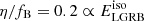
We have two apparent free parameters to determine, fB and η. For simplicity, we assumed that both parameters are constants. We can then use observations of luminous LGRBs from the SHOALS survey to calibrate the ratio  such that the peak of the modeled isotropic-equivalent energy distribution matches the observed one. In Fig. 3 we show the result of this calibration, namely η/fB = 0.2. With this constraint, we can choose reasonable values of fB and obtain a corresponding η. Under certain model assumptions, the jet opening angle can be estimated from the afterglow (Sari et al. 1999; Frail et al. 2001) or the prompt emission of LGRBs (Goldstein et al. 2016), with mean reported values being roughly in the range of 3 to 20 degrees (corresponding to fB of 0.001-0.06). For our fiducial model we chose fB = 0.05 and η = 0.01. Different choices of fB, given the calibration, result in different LGRB rate densities as shown in Fig. C.1. Lower fB values lead to a suppression of the rates as the chance of seeing these systems is directly proportional to fB, while the contrary is true for larger fB values.
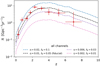 |
Fig. C.1. Modeled luminous LGRB rate densities as a function of redshift for all channels combined. The figure illustrates model uncertainties given an arbitrary choice of beaming fraction fB ∈ [0.01, 0.03, 0.05, 0.1]. The LGRB energy efficiency, η, is obtained from the isotropic-equivalent energy calibration condition η/fB = 0.2. |
Appendix D: BBH and LGRB rate densities and detection rate
The BBH merger rate density, ℛBBHs(z), is the number of BBH mergers per comoving volume per year as a function of redshift. This quantity can be calculated (Bavera et al. 2022) by convolving the redshift- and metallicity-dependent SFR density with the synthetic BBH population obtained by sampling initial binary distributions. To conduct this calculation, we assumed a flat Λ cold dark matter (CDM) cosmology with H0 = 67.7 km s−1 Mpc−1 and Ωm = 0.307 (Planck Collaboration XIII 2016).
We assumed a modeled redshift- and metallicity-dependent SFR, SFR(z, log10(Z)), from the TNG100 Illustris simulation (Nelson et al. 2019). Illustris is a state-of-the-art large-scale cosmological simulation of the Universe. This model tracks the expansion of the Universe assuming a flat ΛCDM cosmology, the gravitational pull of baryonic and dark matter onto itself, the hydrodynamics of cosmic gas, and the formation of stars. The simulated comoving volume of (100Mpc)3 contains tens of thousands of galaxies captured in high detail. Illustris is calibrated to match the present-day ratio of the number of stars to dark matter for galaxies of all masses and the total amount of star formation in the Universe as a function of time. Furthermore, the simulation also matches the galaxy stellar mass and luminosity functions.
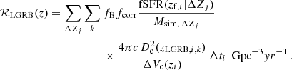
The population synthesis predictions are performed in finite time bins of Δti = 100 Myr and log-metallicity bins ΔZj. Each binary k with BH masses m1, k and m2, k is placed at the redshift of formation zf, i, which corresponds to the center of Δti, and merges at redshift zm, i, k for its corresponding metallicity bin of ΔZj. The BBH rate density is given by the Monte Carlo sum (Bavera et al. 2022)
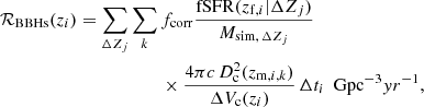
where Msim, ΔZj is the simulated mass per log-metallicity bin, ΔZj, and fcorr is the normalization constant that converts the simulated mass to the total stellar population (Bavera et al. 2020). Here, fSFR(z|ΔZj) = ∫ΔZjSFR(z, log10(Z))log10Z is the fractional SFR density corresponding to the log-metallicity bin ΔZj and ΔVc(zi) is the comoving volume shell corresponding to Δti,
where, Δzi is the redshift interval corresponding to the formation time bin Δti,  is the comoving distance,
  and ΩΛ = 1 − Ωm.
A fraction of merging BBHs emit LGRBs at the compact object’s formation (i.e.,  where the dummy index l = 1, 2 indicates the first- or second-formed BH). In the case of CE and SMT channels, only the second-born tidally spun-up BH can lead to an LGRB event, while for the CHE channel we assume both stars can emit the LGRB at the same time
  . We can therefore compute the LGRB rate density, RLGRB(z), by substituting zLGRB, i, k for zm, i, k in Eq. (D.1). Accounting for beaming, we obtain the LGRB rate density visible to an observer as
To highlight the uncertainties in the SFR density and metallicity distribution, which might bias our rate estimate, we compare our results given the fiducial SFR density choice (IllustrisTNG, Nelson et al. 2019) to an alternative SFR density (Madau & Fragos 2017) assumed in previous works (Bavera et al. 2020, 2022), where it was assumed that metallicity follows a truncated log-normal distribution around the empirical mean of Madau & Fragos (2017) with σ = 0.5 dex. In Fig. D.1, we see that IllustrisTNG SFR density peaks at slightly higher redshift z ∈ [2, 3] compared to tge Madau & Fragos (2017) SFR density, which peaks at z = 2, and that the latter shows a larger suppression at higher redshifts. Moreover, the alternative model predicts twice the fiducial BBH rate densities for z < 2. The difference lies in the metallicity distribution which in the alternative model predicts more low metallicity systems compared to the IllustrisTNG metallicity distribution. This difference is due to the truncation of the log-normal distribution centered around the empirical mean which shifts the distribution toward lower metallicity systems and, hence, leads to an overproduction of merging BBH systems compared to IllustrisTNG.
 |
Fig. D.1. Modeled merging BBH (dashed lines) and luminous LGRB (solid lines) rate densities as a function of redshift, for all channels and for their combination. The figure illustrates model uncertainties given an alternative choice of SFR density (Madau & Fragos 2017) (dashed gray line) which is assuming that metallicities follows a truncated log-normal metallicity with σ = 0.5 dex as in Bavera et al. (2020, 2022), in blue, versus the fiducial assumption of the IllustrisTNG SFR density (Nelson et al. 2019) (solid gray line), in black. The fiducial luminous LGRB rate estimate assumes the beaming fraction fB = 0.05 and LGRB energy efficiency η = 0.0.01, while the alternative model was calibrated against the empirical isotropic-equivalent energy to fB = 0.02 and η = 0.002. |
The BBH detection rate RBBHs is the number of BBH mergers observed per year by a GW detector network. Similarly to the rate density calculation, we can calculate the BBH detection rate with the Monte Carlo sum (Bavera et al. 2022)
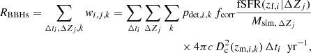
where wi, j, k is the contribution of the BBH k to the detection rate. Similarly to the rate density calculation, the binary, k, is placed at the time bin Δti, whose center is the redshift of formation, zf, i, and merges at zm, i, k for its corresponding metallicity bin, ΔZj. Here, pdet, i, k ≡ pdet(zm, i, k, m1, k, m2, k, a1, k, a1, k) is the detection probability, which accounts for selection effects of the detector. Each BBH k is characterized by the masses m1, k and m2, k and by the dimensionless spin vectors a1, k and a2, k. To compute pdet, i, k (Bavera et al. 2022), we assumed a three-detector configuration with a network signal-to-noise ratio threshold of 12 and “mid-high–late-low” sensitivity (Abbott et al. 2018), consistent with the third observing run of the LIGO and Virgo detectors (Bavera et al. 2022; Zevin et al. 2021).
The normalized weight 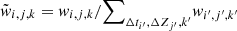 was used to generate the observable GW distributions of the detected BBH modeled population shown in the left panel of Fig. 1. To generate the underlying (intrinsic) BBH merging distribution in Fig. 1 (i.e., what a detector on Earth with infinite sensitivity would observe), we weighted the modeled population with
  . Finally the intrinsic distribution of BBH mergers associated with luminous LGRBs shown in the right panel of Fig. 1 was obtain by weighting the modeled population as
Appendix E: Luminous LGRB evidence in GWTC-2
The probability of a GW event x having emitted a luminous LGRB, given our model, is calculated as
where we approximated the integrals with a Riemann sum over the finite l and m bins of size Δχeff = 0.05 and ΔMchirp = 2 M⊙, respectively. The GW events’ posterior probability density, p(χeff, Mchirp|x), is discretised and calculated at the center of each 2D bin ( ). Here, fLGRB is the probability density of an event with (χeff,Mchirp) having emitted a luminous LGRB at BBH formation. We approximate this probability, given our model, over the finite bins
  and
and  as
as
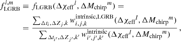
where  is the weight contribution of each binary to the intrinsic detection rate and
  is conditioned against the luminous LGRB criteria similar to Eq. (D.5).
The probability pLGRB of each event in GWTC-2 is summarized in Table E.1, where we also report as a reference the median χeff and Mchirp of each event.
Probabilities of each BBH event in GWTC-2 having emitted a luminous LGRB,  , at the formation of the BBH system. For comparison, we report the median χeff and Mchirp for each event. The estimated number of GWTC-2 events that had emitted a luminous LGRB is ≈4 out of 46.
Appendix F: Metallicity of LGRB progenitors
The maximal ZAMS metallicity of LGRB progenitors in our models is primarily dictated by the interplay of tides and Wolf-Rayet stellar winds (Nugis & Lamers 2000), which is the dominant phase of stellar wind mass loss and is taken to scale with metallicity as ∝(Z/Z⊙)0.85 (Vink et al. 2001). In our model, this threshold is at Zmax ≈ 0.2 Z⊙, where we adopt Z⊙ = 0.017 (Grevesse et al. 1996). As shown in Fig. 4, this corresponds to the lower 16% bound of the metallicity distribution of newly formed stars at z = 2 in the IllustrisTNG simulation, which we used as input in our models. In the same figure we compare the progenitor metallicities of modeled LGRBs to the subsample of the SHOALS LGRBs, which has 45 identified host galaxies that have measured metallicities for z < 2.5 (Graham et al. 2019). We translated the reported 12 + log10(O/H) to [Fe/H] using an empirical relation between [O/Fe] and [Fe/H] (Nicholls et al. 2017) and took the solar reference as [O/H]ref = 8.83 (Grevesse & Sauval 1998). Explicitly, we numerically solved the equation [Fe/H]=[O/H]−[O/Fe]([Fe/H]) with respect to [Fe/H], where [O/H] = 12 + log10(O/H) − [O/H]ref and (see Eq. (5) in Nicholls et al. 2017)
![$$ \begin{aligned}[\mathrm{O/Fe} ]\left([\mathrm{Fe/H} ]\right) = {\left\{ \begin{array}{ll} +0.5, \,&-2.5 < [\mathrm{Fe/H} ] \le -1 \\ -0.5 \times [\mathrm{Fe/H} ], \,&-1 < [\mathrm{Fe/H} ] \le 0.5 \\ -0.25, \,&[\mathrm{Fe/H} ] > 0.5 \, . \end{array}\right.} \end{aligned} $$](/articles/aa/full_html/2022/01/aa41979-21/aa41979-21-eq30.gif)
Typical values of [O/Fe] increase as [Fe/H] decreases due to the increased influence of Type II supernovae over Type Ia at lower metallicities. At face value, we find that 40% of the observed LGRB host galaxies have metallicities lower than Zmax. However, when taking possible systematic uncertainties in the calibration of different metallicity measurement methods into account, we find that our model can be consistent for between 18% and 86% of all observed luminous LGRBs (cf. Fig. 4). These uncertainties can be as high as ±0.35 dex on the measured abundance log10(O/H) (Kewley & Ellison 2008), where Graham et al. (2019) determined metallicities using the R23 diagnostic scale of Kobulnicky & Kewley (2004) which are skewed toward larger values with respect to other calibration methods (cf. Fig. 2 of Kewley & Ellison 2008).
All Tables
Probabilities of each BBH event in GWTC-2 having emitted a luminous LGRB, , at the formation of the BBH system. For comparison, we report the median χeff and Mchirp for each event. The estimated number of GWTC-2 events that had emitted a luminous LGRB is ≈4 out of 46.
All Figures
|
Fig. 1. Joint distribution of the chirp mass, Mchirp, and the effective inspiral spin parameter, χeff, for the combined CE, SMT, and CHE channels. For both sub-figures, the model predictions for the underlying (intrinsic) BBH population are shown in gray, where lighter shades represent larger contour levels of 90% and 99.9%, respectively. Left: detected BBH population with O3 sensitivity, shown in orange. Overlaid in black are the O1, O2, and O3a of the LIGO Scientific and Virgo Collaboration (LVC) GWTC-2 (Abbott et al. 2021a) data with their 90% CIs; GW190521 is outside the plotted window. Right: BBH subpopulation that emitted LGRBs at BBH formation, shown in blue. The ten events in GWTC-2 with chances > 10% of having emitted a luminous LGRB at BBH formation are indicated in black. The two events with > 50% probabilities, GW190517 and GW190719, are indicated with star markers. No bin smoothing was applied when constructing the contour levels. |
| In the text | |
|
Fig. 2. Modeled merging BBH and luminous LGRB rate densities as a function of redshift from isolated binary evolution in dashed and solid black lines, respectively. The CE, SMT, and CHE channel contributions are indicated in orange, blue, and green colors, respectively. The violet marker denotes observable constraints of local BBH rate densities at z = 0 from LVC GWTC-2 (Abbott et al. 2021a) and the red markers the luminous LGRB rate densities from the SHOALS survey (Perley et al. 2016). The SHOALS survey LGRB rate densities are not beaming-corrected and hence probe the observed and not the intrinsic LGRB population. Our fiducial model assumes LGRB efficiency η = 0.01, constant beaming factor fB = 0.05, and IllustrisTNG redshift- and metallicity-dependent star formation rate (Nelson et al. 2019). |
| In the text | |
|
Fig. 3. Normalized histogram of the observed luminous LGRB isotropic-equivalent energies with redshift z < 5 from the SHOALS survey, in light red, compared to the modeled LGRB isotropic-equivalent energies. Our fiducial model was calibrated such that the modeled LGRB energies peak near the observed energy distribution. This is achieved for |
| In the text | |
|
Fig. 4. Cumulative distribution function (CDF) of the modeled LGRB progenitors’ metallicities for redshifts z < 2.5, in blue. The CDF of the observed SHOALS LGRB host galaxy metallicities for z < 2.5 (Graham et al. 2019) are indicated in orange. The light orange shaded area shows the uncertainty in the observed CDF due to systematic offsets in the measurement of log10(O/H), depending on the calibrations used, and the stellar mass of the galaxy which can be as high as Δ[log10(O/H)] ≈ 0.7 dex (Kewley & Ellison 2008). As a reference, we indicate with a vertical dashed black line the median metallicity from the IllustrisTNG simulation at redshift z = 2, and lighter gray shaded areas delineate larger CIs of 68%, 95%, and 99% for the assumed star formation metallicity distribution. |
| In the text | |
|
Fig. C.1. Modeled luminous LGRB rate densities as a function of redshift for all channels combined. The figure illustrates model uncertainties given an arbitrary choice of beaming fraction fB ∈ [0.01, 0.03, 0.05, 0.1]. The LGRB energy efficiency, η, is obtained from the isotropic-equivalent energy calibration condition η/fB = 0.2. |
| In the text | |
|
Fig. D.1. Modeled merging BBH (dashed lines) and luminous LGRB (solid lines) rate densities as a function of redshift, for all channels and for their combination. The figure illustrates model uncertainties given an alternative choice of SFR density (Madau & Fragos 2017) (dashed gray line) which is assuming that metallicities follows a truncated log-normal metallicity with σ = 0.5 dex as in Bavera et al. (2020, 2022), in blue, versus the fiducial assumption of the IllustrisTNG SFR density (Nelson et al. 2019) (solid gray line), in black. The fiducial luminous LGRB rate estimate assumes the beaming fraction fB = 0.05 and LGRB energy efficiency η = 0.0.01, while the alternative model was calibrated against the empirical isotropic-equivalent energy to fB = 0.02 and η = 0.002. |
| In the text | |
Current usage metrics show cumulative count of Article Views (full-text article views including HTML views, PDF and ePub downloads, according to the available data) and Abstracts Views on Vision4Press platform.
Data correspond to usage on the plateform after 2015. The current usage metrics is available 48-96 hours after online publication and is updated daily on week days.
Initial download of the metrics may take a while.