| Issue |
A&A
Volume 665, September 2022
|
|
|---|---|---|
| Article Number | A59 | |
| Number of page(s) | 13 | |
| Section | Extragalactic astronomy | |
| DOI | https://doi.org/10.1051/0004-6361/202243724 | |
| Published online | 09 September 2022 | |
The χeff − z correlation of field binary black hole mergers and how 3G gravitational-wave detectors can constrain it
1
Département d’Astronomie, Université de Genève, Chemin Pegasi 51, 1290 Versoix, Switzerland
e-mail: This email address is being protected from spambots. You need JavaScript enabled to view it.
2
Gravitational Wave Science Center (GWSC), Université de Genève, 1211 Geneva, Switzerland
3
Center for Interdisciplinary Exploration and Research in Astrophysics (CIERA) and Department of Physics and Astronomy, Northwestern University, 1800 Sherman Ave, Evanston, IL 60201, USA
4
Kavli Institute for Cosmological Physics, The University of Chicago, 5640 South Ellis Avenue, Chicago, IL 60637, USA
5
Enrico Fermi Institute, The University of Chicago, 933 East 56th Street, Chicago, IL 60637, USA
6
IAASARS, National Observatory of Athens, Vas. Pavlou and I. Metaxa, Penteli 15236, Greece
Received:
6
April
2022
Accepted:
19
June
2022
Abstract
Understanding the origin of merging binary black holes is currently one of the most pressing quests in astrophysics. We show that if isolated binary evolution dominates the formation mechanism of merging binary black holes, one should expect a correlation between the effective spin parameter, χeff, and the redshift of the merger, z, of binary black holes. This correlation comes from tidal spin-up systems preferentially forming and merging at higher redshifts due to the combination of weaker orbital expansion from low metallicity stars given their reduced wind mass loss rate, delayed expansion and have smaller maximal radii during the supergiant phase compared to stars at higher metallicity. As a result, these tightly bound systems merge with short inspiral times. Given our fiducial model of isolated binary evolution, we show that the origin of a χeff − z correlation in the detectable LIGO–Virgo binary black hole population is different from the intrinsic population, which will become accessible only in the future by third-generation gravitational-wave detectors such as Einstein Telescope and Cosmic Explorer. Given the limited horizon of current gravitational-wave detectors, z ≲ 1, highly rotating black hole mergers in the LIGO–Virgo observed χeff − z correlation are dominated by those formed through chemically homogeneous evolution. This is in contrast to the subpopulation of highly rotating black holes in the intrinsic population, which is dominated by tidal spin up following a common evolve event. The different subchannel mixture in the intrinsic and detected population is a direct consequence of detector selection effects, which allows for the typically more massive black holes formed through chemically homogeneous evolution to be observable at larger redshifts and dominate the LIGO–Virgo sample of spinning binary black holes from isolated evolution at z > 0.4. Finally, we compare our model predictions with population predictions based on the current catalog of binary black hole mergers and find that current data favor a positive correlation of χeff − z as predicted by our model of isolated binary evolution.
Key words: gravitational waves / black hole physics / binaries / close
© S. S. Bavera et al. 2022
 Open Access article, published by EDP Sciences, under the terms of the Creative Commons Attribution License (https://creativecommons.org/licenses/by/4.0), which permits unrestricted use, distribution, and reproduction in any medium, provided the original work is properly cited.
This article is published in open access under the Subscribe-to-Open model. This email address is being protected from spambots. You need JavaScript enabled to view it. to support open access publication.
1. Introduction
The detection of gravitational waves (GWs) from coalescing binary black holes (BBHs) by the LIGO–Virgo–KAGRA (LVK) Collaboration has opened a new window for the study of stellar and binary astrophysics (Aasi et al. 2015; Acernese et al. 2015; Akutsu et al. 2021). To date, the LVK Collaboration has reported 69 BBH events with a false alarm rate (FAR) smaller than 1 yr−1 (Abbott et al. 2019, 2021a,b,c). However, after more than half a decade since the first detection of GWs, the origin of merging BBHs remains an open question. This is not due to a lack of theoretical predictions, but rather because of the degeneracy between different formation channel model predictions and unconstrained astrophysical processes of these models (see, e.g., Mandel & Broekgaarden 2022; Zevin et al. 2021).
The improved sensitivity of the LVK detectors and planned third-generation (3G) GW detectors such as the Einstein Telescope (Punturo et al. 2010) and the Cosmic Explorer (Reitze et al. 2019) will increase BBH detection rates by orders of magnitude. A larger sample size would allow for detailed investigations of correlations between BBH observable properties (e.g., Maggiore et al. 2020; Tiwari 2022), which might enable different astrophysical formation channels to be distinguished. For example, multiple studies have looked for potential correlations between masses and redshifts (Fishbach et al. 2021; Abbott et al. 2021d), Mchirp − χeff (Safarzadeh et al. 2020; Abbott et al. 2021d; Franciolini & Pani 2022), χeff − q (Callister et al. 2021a; Abbott et al. 2021d), and χeff − z (Biscoveanu et al. 2022). The redshift at which the BBH systems merge, z, is a proxy for the distance to the source, Mchirp = (m1m2)3/5/(m1 + m2)1/5 is the chirp mass where m1 and m2 are the BH component masses, q = m2/m1 is the mass ratio defined with m2 < m1, and  is the effective spin parameter where a1 and a2 are the component BH dimensionless spin vectors and
  the orbital angular momentum unit vector.
Here, we demonstrate that field-formed BBHs naturally predict a χeff − z correlation. Under the assumptions of efficient angular momentum transport inside stars, supported by asteroseismological observational constraints (Kurtz et al. 2014; Deheuvels et al. 2014; Gehan et al. 2018) and current GW observations (Belczynski et al. 2020; Zevin et al. 2021), as well as Eddington limited mass accretion efficiency onto BHs, the origin of BH spin in field BBHs arises from tidal interactions during the late BH–Wolf-Rayet (BH-WR; Qin et al. 2018; Bavera et al. 2020; Fuller & Lu 2022) or WR-WR (Hotokezaka & Piran 2017; Olejak & Belczynski 2021) evolutionary phases; or, alternatively, through chemically homogeneous evolution induced by rotational mixing caused from tidal spin-up during the early evolutionary stage of close binaries (Mandel & de Mink 2016; Marchant et al. 2016). From first principles, such correlation should exist since the strength of tidal interaction steeply depends on the orbital separation (Zahn 1977; Hut 1981) and the distribution of orbital separation pre-core collapse evolves with redshift. The redshift evolution of the orbital separation distribution originates from the metallicity-dependent stellar winds (Nugis & Lamers 2000; Vink et al. 2001), whose intensity increases as a function of metallicity. Stronger wind-mass loss (during the BH-WR binary evolution phase) widens the binary more efficiently, inhibiting or even canceling the effects of tides. Because the mean metallicity of the Universe decreases as a function of redshift (Madau & Dickinson 2014; Madau & Fragos 2017), the empirical expectation would call for an increasing fraction of BBH mergers with highly spinning BH components from tidal spin up as a function of redshift. Additionally, low-metallicity stars are more compact at zero age main sequence (ZAMS), expanding later in their evolution and having smaller maximal radii during the supergiant phase, as compared to stars at a higher metallicity.
In this paper, we discuss the evolving χeff distribution as a function of redshift for field BBHs from the common envelope (CE), stable mass transfer (SMT), and the chemically homogeneous evolution (CHE) channels. The paper is structured as follows. First, we introduce our fiducial model and describe how we quantify the χeff − z correlation in Sect. 2. In Sect. 3, we present the redshift evolution of the χeff distribution for the intrinsic and detectable BBH population, as predicted by our model of isolated binary evolution. We then compare our model predictions against the LIGO–Virgo catalog of BBHs. In Sect. 4, we discuss how potential uncertainties in our model might affect the χeff distribution of field BBHs and how a possible change in the mixing fraction of the different channels predicted from isolated binary evolution might impact our results. Our findings are summarized in Sect. 5.
2. Methods
2.1. Binary black-hole population synthesis model
This study uses the isolated binary evolution model presented in Bavera et al. (2022a), calculated using the POSYDON framework (Fragos et al. 2022), which accounts for BBH formation through the CE, SMT, and CHE channels. It has been shown that this model (i) leads to BBH observable properties consistent with the events of the second LIGO–Virgo GW transient catalog (GWTC-2; Zevin et al. 2021); (ii) have BBH merger rate estimates compatible with the observational constraints of GWTC-2 – and now GWTC-3 (Bavera et al. 2021a); (du Buisson et al. 2020); (iii) the subpopulation of highly spinning BBHs might explain the observed population of luminous LGRBs across the cosmic history of the Universe (Bavera et al. 2022a); and (iv) does not violate current upper limit estimates of the stochastic GW background (Bavera et al. 2022b).
In contrast to most rapid population synthesis studies, our simulations accurately model the late tidal spin-up phase of the second-born BH and CHE due to rotational-induced mixing of tidally spun-up ZAMS binaries. The former is done by following the evolution of the binaries from ZAMS up to the formation of the BH-WR systems after the second mass transfer phase with the rapid population synthesis code COSMIC (Breivik et al. 2020) and then uses detailed MESA (Paxton et al. 2011, 2013, 2015; Paxton et al. 2018, 2019) BH-WR simulations (Bavera et al. 2021a) to accurately model the final tidal spin-up phase of the BH-WR system up to central carbon exhaustion of the WR star, as done in Bavera et al. (2022a). The detailed BH-WR simulations self-consistently model the angular momentum evolution of the WR star, which is determined by the interplay of tides, WR stellar wind mass loss, and the evolution of the WR stellar structure.
Massive stars in short orbital periods (p < 2 days) at ZAMS with nearly equal masses tidally spin up to become highly rotating bodies, which induces rotational mixing and eventually leads to CHE. Because COSMIC cannot model the parameter space leading to CHE, as the code cannot accurately follow the back-reaction on the stellar structure and evolution from rotationally induced mixing, CHE is carried out by matching ZAMS binary conditions to detailed MESA simulations targeting CHE according to du Buisson et al. (2020), as implemented in Bavera et al. (2022a).
Given the availability of the stellar profile at carbon exhaustion from the MESA simulations, in both cases, the core collapse considers disk formation during the collapse of highly spinning stars. Additionally, we account for mass loss through neutrinos, pulsational pair-instability and pair-instability supernovae (PPISNe & PISNe; Marchant et al. 2019), and orbital changes resulting from anisotropic mass loss and isotropic neutrinos mass loss (Kalogera 1996), as explained in Appendix D of Bavera et al. (2021a). Because we implement the Fryer et al. (2012) delayed collapse mechanism which assigns zero velocity kicks to collapsing stars with carbon-oxygen cores with masses above 11 M⊙, in practice, we find a statistically small number of systems with χeff < 0. Alternatively, non-negligible kicks would lead to a more considerable fraction of negative χeff (see, e.g., Rodriguez et al. 2016; Gerosa et al. 2018; Callister et al. 2021b; Stevenson 2022). For a detailed explanation of the main features and the physical assumptions made in this model, we refer the reader to the extensive discussions in Bavera et al. (2022a).
2.2. Detection rates
Merger rates are computed by convolving the redshift- and metallicity-dependent star formation rate as predicted by the Illustris-TNG simulation (Nelson et al. 2015) with the synthetic catalog of merging BBHs obtained by evolving initial ZAMS conditions at different discrete metallicities with POSYDON. Following the notation of Bavera et al. (2020), 2021a, 2022a), the BBH detection rate of a GW detector network can be expressed as a Monte Carlo sum over the synthetic population of merging BBHs, that is, Rdet = ∑i, j, kwi, j, k(pdet) yr−1, where wi, j, k is the weighted contribution of a binary, k, forming at redshift, zf, i, and merging at redshift zm, k ≡ zk. Here, the dummy index, j, indicates the discrete sum over the 30 simulated log-binned metallicity intervals, ΔZj. The synthetic BBH population is distributed across the cosmic history of the Universe in the center of time bins of size Δti = 100 Myr with the center at the formation redshift zf, i. We chose the time bin size to be small enough to ensure the convergence of our results (see Appendix D of Bavera et al. 2022a for the details of the calculation).
To compute the BBH detection rate of LIGO–Virgo, we account for the detectors’ selection effects, pdet, given the source redshift, BH masses, and spins. Here, we assume a GW detector network configuration composed by LIGO Hanford, LIGO Livingston, and Virgo at O3 mid-high (late-low) sensitivity (Abbott et al. 2018) with a network signal-to-noise ratio (S/N) threshold of 12 as implemented in Bavera et al. (2021a).
We also consider the sensitivity of the future 3G ground-based GW detector Einstein Telescope. To approximate the BBH detection rate of the Einstein Telescope, we account for detector selection effects given the source redshift and BH masses assuming a theorized noise-sensitive curve ET-D (Hild et al. 2011) as implemented by Barrett et al. (2018) in COMPAS (Team COMPAS 2022). Here, we assume a conservative S/N threshold of 12 for the Einstein Telescope, similar to what Hild et al. (2011) assumed. In practice, we find that this assumption sets the horizon of a BBH with m1 = m2 = 15 M⊙ at z = 10, namely  .
.
Finally, we will distinguish the intrinsic detection rate, i.e., what a GW detector with infinite sensitivity would observe on Earth, using the notation w̃i,j,k = wi,j,k(pdet = 1), as first introduced in Bavera et al. (2022a).
2.3. Relative channel contribution
Once detection rates are defined, we can compute the relative contribution to the intrinsic detection rate from each one of the isolated binary evolution channels (CE, SMT, and CHE) at a given redshift as:
 (1)
(1)
where z ∈ [0, 10] is discredited in bins, Δz, taken to have a constant cosmic time width of Δt = 200 Myr. Similarly, for the detectable population, we define  , where we use wi, j, k instead of w̃i,j,k in z ∈ [0, 1] for LIGO–Virgo and z ∈ [0, 10] for the Einstein Telescope.
2.4. Quantifying the χeff − z correlation
To quantify the redshift evolution of the χeff distribution, we define fχeff > χ0(z) to be the fraction of merging BBHs with χeff above the arbitrary value, χ0, at a given redshift for the modeled intrinsic BBH population. This quantity is calculated as:
 (2)
(2)
and, similarly, for the detectable populations, we define  with the same redshift spacing and bounds as in Eq. (1).
3. Results
We investigated the χeff − z correlation of field-formed BBHs and assert its detectability given current and planned GW observatories. We first looked at the intrinsic and detectable χeff distributions as a function of redshift in our fiducial model, which includes a potential contribution from the CE, SMT, and CHE channels described in Sect. 3.1. We then quantified the intrinsic and detectable χeff − z correlation by computing the quantities fχeff > χ0(z) and  and the relative channel contributions fchannel(z) and
  , described in Sect. 3.2. Finally, we looked for evidence of the modeled fχeff > χ0(z) and
  in LIGO–Virgo GWTC-3 data, given in Sect. 3.3.
3.1. χeff distribution of field BBHs
First, we show the χeff distribution as a function of discrete redshift bins for the intrinsic and detectable BBH populations in Fig. 1. At low redshifts, the intrinsic distribution manifests a peak at χeff = 0 plus an almost flat distribution up to χeff ≃ 0.5, which then progressively decays. Similarly, the detectable LIGO–Virgo χeff distribution also exhibit a similar narrow peak at χeff = 0. However, in contrast to the intrinsic distribution, we observe a second broader peak at around χeff ≃ 0.35 with an elongated tail reaching large χeff depending on redshift. Both distributions evolve with redshift; with the χeff distribution in the intrinsic population showing a slow evolution with redshift, while in the LIGO–Virgo observable population the distribution evolves significantly over the redshift range between 0 and 1. The median  value of the intrinsic distribution grows from
 ![Mathematical equation: $ \bar{\chi}_{\mathrm{eff}}^{z\in[0,1]}\simeq 0.12 $](/articles/aa/full_html/2022/09/aa43724-22/aa43724-22-eq12.gif) to
to ![Mathematical equation: $ \bar{\chi}_{\mathrm{eff}}^{z\in[5,6]} \simeq 0.33 $](/articles/aa/full_html/2022/09/aa43724-22/aa43724-22-eq13.gif) , while for the LIGO–Virgo detectable population the model predicts that
, while for the LIGO–Virgo detectable population the model predicts that ![Mathematical equation: $ \bar{\chi}_{\mathrm{eff}}^{z\in[0,0.2]}\simeq 0.13 $](/articles/aa/full_html/2022/09/aa43724-22/aa43724-22-eq14.gif) grows to
grows to ![Mathematical equation: $ \bar{\chi}_{\mathrm{eff}}^{z\in[0.8,1]}\simeq 0.41 $](/articles/aa/full_html/2022/09/aa43724-22/aa43724-22-eq15.gif) .
.
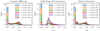 |
Fig. 1. Effective spin parameter, χeff, distribution of field BBHs as a function of redshift, z. Left: modeled intrinsic (underlying) population of field merging BBHs. Center: modeled detectable LIGO–Virgo BBH population assuming simulated O3 detector sensitivity selection effects. Right: modeled Einstein Telescope detectable BBH population assuming a forecast detector sensitivity as in Hild et al. (2011). In all cases, the fraction of non-spinning BBHs decreases as a function of redshift, shifting the χeff distribution to larger χeff values. |
The origin of the redshift evolution of the χeff distribution is different between the intrinsic and the detectable LIGO–Virgo BBH populations as they probe different redshift horizons, z ∈ [0, ∞] and z ∈ [0, 1], respectively. The former encapsulates all merging BBHs at any redshifts and probes the increasing fraction of systems experiencing tidal spin up prior to BBH formation at increasing redshifts (see Sect. 1). In contrast, the detectable LIGO–Virgo population is biased by the BBH mass-dependent selection effects. More massive BHs can be detected at further distances than lighter BHs. We note that at the highest redshifts detectable by LIGO–Virgo (z ≃ 1), only systems with large positive values of χeff are detected due to the increased duration of the inspiral and therefore the S/N. However, the impact of χeff on detectability is minor compared to mass selection effects (Ng et al. 2018).
In the following section, we show how the different evolutionary channels CE, SMT, and CHE, which have distinct spin distributions, are characterized by different detector horizons due to their inherent mass spectrum. For a discussion about the intrinsic and LIGO–Virgo observable joint distributions of χeff vs. Mchirp, we refer to Fig. 1 of Bavera et al. (2022a). Finally, because the Einstein Telescope has a much more distant horizon than current generation GW detectors, the planned GW observatory will be able to detect the majority of the underlying BBH population up to large redshifts, see e.g., z ∈ [4, 5] in Fig. 1. We therefore find that the Einstein Telescope will observe an evolving χeff distribution similar to the intrinsic one.
3.2. χeff − z correlation of field BBHs
The χeff − z correlation of field BBHs in the intrinsic population, fχeff > χ0(z), is shown in the leftmost column of Fig. 2 for χ0 = 0.2 and χ0 = 0.5. In both cases, fχeff > χ0(z) is monotonically increasing and reaches an asymptotic plateau at high redshifts, z > 5 and z > 8 for χ0 = 0.2 and χ0 = 0.5, respectively. To understand the origin of the fχeff > χ0(z) shape, we need to look at this quantity channel-wise and consider the relative contribution of each channel fchannel(z) to the total BBH intrinsic population. In Fig. 2, we can see that at low redshifts the intrinsic BBH merging population is composed of a mix of channels, fCE(z = 0)=30%, fSMT(z = 0)=55%, and fCHE(z = 0)=15%. In contrast, at higher redshifts, the total population of merging BBHs is dominated by the CE channel, with fCE(z ≥ 2)≥80%.
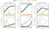 |
Fig. 2. Fractions of BBHs with fχeff > 0.2 and fχeff > 0.5 as a function of redshift (solid lines), and the relative contribution of each field BBH channel, fchannel, according to the legend (dashed lines). Black solid lines show the fraction of systems that satisfy a given χeff criteria for the combined CE, SMT, and CHE channels with redshift-dependent branching fractions accounted for. Left: modeled intrinsic (underlying) population of field merging BBHs. Center: modeled LIGO–Virgo detectable BBH population assuming simulated O3 detector sensitivity selection effects. Right: modeled Einstein Telescope detectable BBH population assuming forecast detector sensitivity as in Hild et al. (2011). In most cases, the fraction of highly spinning BBHs increases as a function of redshift. |
Channel-wise, we can see that  increases monotonically due to a larger fraction of systems experiencing tidal spin-up as a function of redshift. On average, at higher redshifts, binary systems are born at lower metallicities and experience reduced stellar wind mass loss. Hence, an increased fraction of binaries can maintain short orbital separations and tidal locking during the BH-WR phase. A similar argument can be made for the SMT channel. However, because SMT leads, on average, to wider BH-WR orbital separations than the CE channel (Bavera et al. 2021a), we can find
  for any redshift. Moreover, we find that at low redshifts
  , which steadily increases to
  . On the contrary,
  manifests a monotonically decreasing behavior. At low redshifts,
  , that is, all BBHs from the CHE channel are fast spinning, while at higher redshifts most systems possess negligible χeff, with
  . We also notice that highly rotating CHE systems with χeff > 0.5 are not present in the local universe
  but their presence peaks at
  before decreasing again to
  . The decreasing fraction of highly rotating CHE systems as a function of redshift is a direct consequence of angular momentum loss due PPISNe. The CHE channel only operates at low metallicities (Z < 5 × 10⁻³) but only binaries with metallicities Z ≤ 10−4 experience mass loss due to PPISNe (in the considered ZAMS primary masses range ≤150 M⊙). During these pulses, the mass ejection from the stellar surface depletes the angular momentum content of these stars and leads to slowly rotating BHs (see Appendix A for more details). Since at high redshifts (z > 3) the metallicity-dependent star formation rate leads to an increasing relative fraction of extremely low metallicity binaries, we expect to observe a decreasing
  as a function of increasing redshift. The three channels combined lead to the monotonically increasing behavior of fχeff > χ0(z) we see in Fig. 2, which is mainly dominated by the CE channel. In Appendix B, we show how our fiducial model predictions would change if one of these three channels would be neglected, see Sect. 4 for a discussion of these alternative scenarios.
The χeff − z correlation of field BBHs in the detectable populations,  , is shown in the center and right columns of Fig. 2 for LIGO–Virgo detectors at O3 sensitivity and the Einstein Telescope, respectively, for χ0 = 0.2 and χ0 = 0.5. For LIGO–Virgo detectability,
  is a monotonically increasing function growing from
  to
to  , and
, and  to
to  . On the other hand, the Einstein Telescope
  mimics the intrinsic distribution up to z ≃ 5 above which it shows a suppression. The similarity between the Einstein Telescope detectable distribution and the underlying distribution is due to the Einstein Telescope GW horizon being much more distant than that of LIGO–Virgo. The suppression for the detectable Einstein Telescope
  is caused by the fact that the detector cannot resolve all distant low mass highly rotating BBHs formed through the CE channel. To understand the difference between the LIGO–Virgo
  redshift evolution compared to the Einstein Telescope and the intrinsic BBH population, we need to once again consider the relative contribution of each channel. Similarly to the intrinsic distribution, for LIGO–Virgo at low redshift, we have a mixed contribution from the different channels,
  ,
,  , and
, and  . Up to redshift z = 0.4 the SMT channel dominates over CE and CHE, above which the CHE channel dominates the LIGO–Virgo detectable population to the point where
  . This is notably different than the behavior of the intrinsic BBH population and is a direct consequence of selection effects favouring high BH masses. The different channels have different BH mass distributions, which result in different observational horizons for each channel. Notably, the CHE channel leads to more massive BBHs compared to CE and SMT, and hence this channel can be probed by LIGO–Virgo at larger redshifts compared to BBHs formed from the CE and SMT channels. The described signature leads to a bimodal distribution of χeff in the LIGO-Virgo detectable BBH population in Fig. 1. The second peak is mostly composed of BBHs formed through the CHE channel (see Bavera et al. 2022a, for further discussions). This bimodal feature is not present in the χeff distribution of the intrinsic BBH population for z ∈ [0, 1] (see the right panel of Fig. 1). Since, intrinsically,
  ,
,  , and
, and  is monotonically increasing at low redshifts, we also find a monotonically increasing
  function for LIGO–Virgo sensitivity. A similar argument can be made for
  , where for low redshifts, it holds that
  while both
  and
and  are monotonically increasing, which results in
  monotonically increasing. Finally, notice that the CHE dominance is not present in the Einstein Telescope detectable population as the 3G detector, given our theorised sensitivity curve, will be able to observe the entire intrinsic BBH population up to redshift z ≃ 4 − 5.
3.3. Evidence for the χeff − z correlation in GWTC-3 data
Our model provides a falsifiable prediction that both the underlying and detected high-χeff fractions fχeff > χ0(z) and  for the O3 LIGO–Virgo detector network should increase as a function of redshift if isolated evolution channels dominate the BBH merger rate at low redshifts. We notice that at low redshifts, z < 1, the evolution of this fraction for the intrinsic BBH population is mild, but can be amplified by the selection effects of current ground-based detectors. We use BBH events from GWTC-3 to infer both fχeff > χ0(z) and
  and compare them against our model predictions. As in Abbott et al. (2021d), we only consider GWTC-3 events with a false alarm rate (FAR) smaller than 1 yr−1. In GWTC-3, there are 76 events satisfying this condition from which we exclude the binary neutron stars (NSs) GW170817 and GW190425_081805, the NS-BH systems GW190426_152155, GW200105_162426, GW200115_042309, and the events GW190814, GW190917_114630 in which the less massive compact objects exhibit masses that indicate they are either a massive NS or a BH. Our BBH sample therefore includes a total of 69 BBH events.
We first approximated the observed  for O3, or
  , in a model agnostic way directly from the observed events. We measured
  on a sample of 10 000 mock GWTC-3 catalogs composed of 69 BBH events. A mock catalog of events,
  , was generated by drawing a 2D sample,
  , from each event’s xi 2D posterior distribution1p(χeff, z|xi) weighted by the inverse of the prior 2D probability density p(χeff, z) in order to sample from the likelihood. The events’ posterior and prior distributions have been publicly released by the LIGO–Virgo collaboration. We approximated the discretely sampled prior distribution probability density function (PDF) with a 2D kernel density estimator (KDE) trained on the GWTC-3 event samples where the bandwidth of the KDE is set by Scott’s rule (Scott 2015) as implemented in the Gaussian KDE function of the SciPy Python module (Virtanen et al. 2020). The accuracy of our KDE method to represent the inferred 2D distributions is verified by comparing the histogram of the original samples and samples generated from the KDEs.
To perform a fair comparison of our model with the observations, we need to account for (i) the statistical variance of drawing a sample of 69 events from our model and (ii) to account for the measurement uncertainty for BBH parameters. This is done by generating 10 000 mock samples of 69 events from our model, to which we add mock uncertainty to each event. We approximate measurement uncertainties following a procedure first shown in Bavera et al. (2020) for the χeff parameter. Here, we extend this procedure to the 2D case. Mock uncertainties are obtained by shifting another set of 10 000 mock GWTC-3 catalogs by each event’s median value  . When the mock uncertainty is added to the model mock samples, we find that this methodology overestimates the measurement uncertainty of events with low redshift of merger. This occurs because this methodology does not assign smaller measurement uncertainties to events with smaller redshifts of merger. Such a correlation is expected because of the greater measurement uncertainty for more distant events, which is due to their typically smaller S/N compared to events merging at lower redshifts. In practice, we find that this procedure only leads to 0.6% of the sample having nonphysical values |χeff|> 1 and 4.2% of systems having nonphysical z < 0, which we map back to |χeff|=1 or z = 0. We claim that this bias is small and does not affect our results, as we still find that events with larger z̄ have broader χeff distributions.
In Fig. 3, we show the comparison of the median  computed on the sample of mock GWTC-3 catalogs with the model prediction. The GWTC-3 quantity is independently measured for each mock catalog in the interval z ∈ [0, 1] by counting the events meeting the χeff > χ0 condition in the discrete redshift bin Δz with constant cosmic time bin of size of Δt = 1.6 Gyr and then quote the median value at each redshift bin. We can then compare our model predictions with the inclusion of mock uncertainties by overlaying the median and 90% CI
  . We conclude that our model cannot be ruled out given the current GWTC-3 sample. Even though our model 90% CI overlaps with the median inferred GWTC-3 value, a closer comparison with the model median indicates that our model slightly overpredicts the fraction of highly spinning BBHs. This could be due, for instance, to an overprediction of the fraction of highly spinning BBHs formed from the CHE channel which dominates over BBHs formed from the CE channel in the LIGO–Virgo detectable population (see Appendix B) or the existence of an additional channel contributing to the detectable BBH population with small BH spins (see e.g., dynamical formation in globular clusters, Zevin et al. 2021). Other model uncertainties are discussed in Sect. 4.
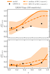 |
Fig. 3. Modeled and observed fractions of BBHs satisfying |


We next infer the underlying fraction fχeff > χ0(z) by fitting a model for the astrophysical BBH population to the GWTC-3 data. We jointly fit the mass (m1, m2), spin χeff, and redshift z distribution, allowing the χeff distribution to evolve redshift but for simplicity neglecting possible correlations between other parameters:
 (3)
(3)
For the mass distribution, p(m1, m2), we use the broken power law model from Abbott et al. (2021e) and for the redshift distribution, p(z), we assume the merger rate evolves as a power law in (1 + z; Fishbach et al. 2018). We model the redshift-dependent spin distribution p(χeff ∣ z) as a mixture model between a “zero-spin” component, approximated as a narrow Gaussian centered at χeff = 0 with standard deviation 0.03, and a “positive spin” component, for which we use a Gaussian distribution 𝒩T with mean 0.2 < μp < 0.5 and standard deviation 0.05 < σp < 0.5 truncated to the range [0, 1] to reflect our model predictions. We take the mixture fraction A between the zero and positive spin components to be a logistic function of z (so that it is always within 0 < A < 1), described by two free parameters, A(z = 0) and A(z = 1). We therefore have
 (4)
(4)
where
 (5)
(5)
with B = A−1(z = 0) − 1 and k = log(A−1(z = 1)−1)−log(B). We fit for all population parameters by sampling from a hierarchical Bayesian likelihood with PyMC3 (Salvatier et al. 2016; and see e.g., Thrane & Talbot 2019; Mandel et al. 2019; Vitale et al. 2022), using the GWTC-3 detector sensitivity estimates covering the first three observing runs and the parameter estimation samples for the GWTC-3 BBH events (LIGO Scientific Collaboration, Virgo Collaboration and KAGRA Collaboration 2019, 2020, 2021a,b,c). We use flat priors on all parameters within their ranges specified above.
The inferred intrinsic χeff population distribution at two redshifts, z = 0 and z = 1, is shown in Fig. 4. At z = 0 the positive-spin component is constrained to be small, whereas at z = 1, the data permit a larger fraction of systems with high χeff, although the overall constraints are more uncertain and more closely resemble the prior. We can directly compare the underlying high-χeff fractions fχeff > 0.2 and fχeff > 0.5 inferred under this fit to the low-redshift z < 1 predictions in the leftmost panel of Fig. 2. In Fig. 5, we show the inferred intrinsic fχeff > 0.2(z) and fχeff > 0.5(z) versus our astrophysical model predictions. The intrinsic fractions are broadly consistent with the model predictions, although the data prefer slightly smaller fractions of large positive χeff at all z, similar to the conclusions of Fig. 3 regarding the observed fractions. To reiterate, this could be due, for instance, to an overprediction of the contribution of the CHE channel (see Appendix B) or the non-negligible contribution of an additional channel with small BH spins. Other model uncertainties are discussed in Sect. 4.
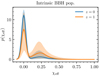 |
Fig. 4. Underlying χeff distribution from fitting the population model of Eq. (4) to the GWTC-3 BBH events. We plot the χeff population distribution at two redshift slices, z = 0 (blue) and z = 1 (orange). Solid lines denote the median and shaded bands denote the 90% CI. |
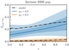 |
Fig. 5. High-χeff fractions in the underlying distribution inferred from the population fit described in Sect. 3.3, in blue and orange according to the legend. Lighter contour colors indicate larger CIs of 50% and 90%, respectively. The fraction of BBH systems with large positive spins in the underlying population may increase with increasing redshift (credibility 82%), consistent with our model predictions (black). We do not yet have enough BBH events at z ∼ 1 to accurately measure the χeff distribution at high z and therefore cannot confidently conclude that the distribution is evolving. |
We verified the goodness-of-fit of the inferred model by performing posterior predictive checks. Figure 6 shows the comparison between the (z, χeff) parameters of ten mock GWTC-3 catalogs versus ten sets of 69 events drawn from the inferred model. This test is analogous to the posterior predictive check in Fig. 2 of Fishbach et al. (2021). Each of the ten sets (plotted with a different marker size) corresponds to one draw from the inferred population hyperposterior. We reweight the single-event posterior from each GWTC-3 event to the population distribution specified by the hyperposterior draw, and draw one (z, χeff) sample per event. We then draw a set of 69 predicted events from the same population distribution, conditioned on detection. We can see that the inferred model sometimes over-predicts the largest observed χeff, while the bulk of both the observed and predicted draws cover an equivalent portion of the z − χeff plane in a comparable abundance, confirming that the inferred model is a good fit to the data.
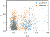 |
Fig. 6. Redshift and effective spin parameters of the 69 confident BBH observations drawn from the GWTC-3 posteriors (orange; “observed”) compared to 69 draws from the inferred distribution fit (blue; “predicted”) described in Sect. 3.3. Each marker shape corresponds to a different set of 69 draws. We plot ten total sets. The inferred model sometimes over-predicts the largest observed χeff, while the bulk of both observed and predicted draws cover an equivalent portion of the z − χeff plane in a comparable abundance, confirming that the inferred model is a good fit for the data. |
Despite the suggestive hint that fχeff > 0.2(z) increases with z, we are not yet able to confidently identify that the χeff distribution varies with redshift under our parameterization. More precisely, we constrain fχeff > 0.2(z = 0.3)> 0.06 at 99% credibility and find that fχeff > 0.2(z) increases with increasing redshift at 82% credibility. Our conclusions are consistent with the results of Biscoveanu et al. (2022), who find that the width of the χeff distribution likely broadens with increasing redshift, but do not find compelling evidence that the mean χeff evolves with redshift2. Our model for field BBH formation predicts that the mean of the χeff distribution must increase with redshift.
We further caution that our phenomenological population fit makes the simplifying assumption that the mass distribution is independent of spin and redshift, despite the fact that we predict a correlation between total mass, χeff, and redshift. However, given current statistical uncertainties on the inferred intrinsic fχeff > χ0(z), we do not expect our systematic errors on this inferred quantity from mismodeling the population distribution to be significant. However, with future data it will be important to allow for χeff to vary with both mass and redshift in BBH population fits, because (as Figs. 1 and 2 show) some of the observed χeff evolution in the LIGO–Virgo catalog will be due to an underlying correlation between χeff and mass. These conclusions are corroborated by Biscoveanu et al. (2022), who find that the preference for χeff to correlate with redshift is stronger than a possible correlation with primary mass, although the two scenarios can be confused for one other.
4. Discussion
In this work, we consider a fiducial model for isolated binary evolution. However, model uncertainties can potentially alter BBH observable distributions and rates (see e.g., Broekgaarden et al. 2022 for an extended overview of such uncertainties). Here, we are interested in astrophysical uncertainties which may alter the χeff − z joint distribution.
Our fiducial model assumes efficient angular momentum transport inside stars, which leads to the formation of non-spinning first-born BHs for the CE and SMT channels. Alternatively, a less efficient angular momentum transport would lead to non-negligible birth spins (see e.g., some model variations in Belczynski et al. 2020) that would consequently raise our estimated fraction of highly spinning BBHs fχeff > χ0(z) as the CE and SMT channels dominate the intrinsic BBH population. Nevertheless, current observations are consistent with low birth spins of ≲0.1 for isolated BHs (Abbott et al. 2021e,d; Miller et al. 2020; Zevin et al. 2021).
In Bavera et al. (2021a), the impact of mass-transfer physics uncertainties on the χeff distribution of BBHs formed from the CE and SMT channels was investigated, accounting for uncertainties in (i) the unknown efficiency of CE ejection in the αCE − λ parametrization (see, e.g., Ivanova et al. 2013, for a review), (ii) the SMT accretion efficiency onto BHs, and (iii) the criteria for mass-transfer stability. The first uncertainty directly impacts the relative fraction of highly rotating BBHs in the CE channel as the αCE parameter approximately linearly scales with the orbital separation post CE. For a wide range of αCE ∈ [0.2, 5], Bavera et al. (2021a) showed that the BBH fraction of systems with χeff > 0.1 formed from the CE channel can vary from 0.54 to 0.82 where the merger rate density might also vary by up to one order of magnitude. Nevertheless, Bavera et al. (2021a) showed how both αCE extremes include a non-zero fraction of tidally spun-up BBHs in the CE channel. The second uncertainty affects the initially negligible spin of the first-born BH of a BBH systems formed through the SMT channel. In the case of highly super-Eddington accretion efficiency onto BHs, Bavera et al. (2021a) showed how a non-negligible fraction of first-born BHs could be spun up due to accretion. However, in such cases, depending on the super-Eddington accretion efficiency, Bavera et al. (2021a) found a suppression of the SMT merger rate density up to two orders of magnitude. This occurs because conservative mass transfer is less efficient than unconservative mass transfer in leading to tight BH-WR systems, leading to less BBH systems that can merge in a Hubble time. Finally, the third uncertainty directly impacts the relative fraction of systems that undergo either stable or unstable mass transfer and, hence, CE or SMT evolution. We now examine how these uncertainties might affect the presented χeff − z correlation.
In the present study, we assumed inefficient CE ejection, namely the model with αCE = 0.5 of Bavera et al. (2021a). A smaller value than what was assumed here would lead to a more significant fraction of tidal spun-up BBHs. Because the CE channel dominates the intrinsic BBH population, such a scenario would increase the predicted quantity fχeff > χ0(z). In contrast, a more efficient assumption for CE ejection would lead to a smaller fraction of systems that are tidally spun up. For the detectable fraction  , we expect this assumption to have a minimal impact, as the detectable population of BBHs is dominated by the SMT and CHE channels. Since Bavera et al. (2021a) showed that at αCE = 5 there is still a fraction of highly rotating BBHs formed from the CE channel with a median
  , we can claim that our model will always display a monotonically increasing fχeff > χ0(z) regardless of the αCE value in the CE parameterization.
Our fiducial model assumed Eddington limited mass-transfer accretion efficiency onto BHs. A super-Eddington accretion efficiency onto BHs would boost the fraction of highly spinning BBHs formed from the SMT channel, and, hence, positively contribute to larger values of fχeff > χ0(z) and  . However, given that the BBH merger rate from the SMT channel (both detected and intrinsic) drops by up to two orders of magnitude compared to our fiducial model when increasing the allowed accretion rate onto BHs (see Table 1 of Bavera et al. 2021a), we would expect a smaller intrinsic contribution to the SMT channel than the one modeled here.
Both uncertainties (i) and (iii) might lead to a smaller relative contribution of the CE channel to the total BBH population than what is assumed here, where the CE channel dominates the fχeff > χ0(z) behavior. Moreover, recent studies employing detailed binary simulations point towards an overestimation of systems evolving through and surviving CEs due to envelope stripping during the CE ceasing earlier than what is assumed in rapid population synthesis codes (Fragos et al. 2019; Quast et al. 2019; Klencki et al. 2021; Marchant et al. 2021; Gallegos-Garcia et al. 2021). Therefore, it is natural to ask ourselves what would happen to the modeled fχeff > χ0(z) fraction if the CE channel is negligible compared to SMT and CHE. In such a scenario, given our model, one would expect that most binaries evolving through CE would either evolve through SMT or successfully emerge from the CE at wider orbital separations. In the first case this would lead to a SMT contribution that is similar or greater than what is modeled here. The second case would lead to a reduced fraction of tidally spun-up CE systems, similarly to the outcome of choosing an efficient αCE values. If the remaining SMT and CHE channels retain a similar fraction of highly spinning BBHs to what is modeled here, we would find fχeff > 0.2(z < 4)≃0.2 this result would eventually decay at larger redshifts while the LIGO–Virgo detectable population would still exhibit a monotonically increasing behavior since the contribution of CE systems to the LIGO–Virgo detectable population is small ( ). In Appendix B, we show how Fig. 2 would change given the omission of the CE channel from our fiducial model. At low redshifts, z < 1, we find that the intrinsic fraction fχeff > 0.2 of this alternative model is still consistent with the 90% CI of GWTC-3 constraints shown in Fig. 5.
Similarly to this last point, we alternatively entertain the idea of what would happen to the χeff − z correlation if either the SMT or CHE channels contributions are negligible. This might happen, for example, if we overestimate the contribution of the initial conditions parameter space at low orbital periods that leads to SMT or CHE evolution. In Appendix B, we show that the presented correlation would still be observed. In both cases we still recover monotonically increasing fractions fχeff > χ0(z) and  . However, we note that the model with the omission of the SMT channel manifests a larger, relatively constant fχeff > 0.2(z < 1)≃0.45 which is inconsistent with the 90% CI of GWTC-3 constraints in Fig. 5 of fχeff > 0.2(z < 0.4)< 0.3. Finally, we find that the model that excludes the CHE channel has both an intrinsic fχeff > χ0 and LIGO–Virgo detectable
  closer to the median GWTC-3 inferred constrains of Figs. 3 and 5.
5. Conclusions
In this paper, we investigate the χeff − z correlation of field-formed merging BBHs. An increasing fraction of highly spinning BBHs as a function of redshift is generally expected. At higher redshifts, stars are formed at lower metallicities, experience weaker stellar wind mass loss, and consequently can maintain their short orbital separations and undergo tidal spin up. We quantified this correlation by the fraction of systems with χeff > χ0 as a function of redshift, fχeff > χ0(z). For our fiducial model of field BBHs, which includes the potential contribution of CE, SMT, and CHE channels, this quantity for χ0 ∈ [0.2, 0.5] shows a monotonically increasing behavior as a function of redshift in the underlying BBH population. We also present predictions for the detectable  for the LIGO–Virgo detector network at O3 sensitivity and the Einstein Telescope. Because of the smaller horizons of current GW detectors (z ≃ 1), the origin of the monotonically increasing LIGO–Virgo
  quantity is different than the intrinsic BBH population or that which the Einstein Telescope will observe in the future. Such differences originate from different BH mass distributions of the various channels. On average, highly rotating BBHs formed from the CHE channel are more massive than tidally spun up BBH systems formed from the CE channel. Hence, LIGO–Virgo detector selection effects favour high BH masses and lead to different observational horizons for different channels. We find that, in contrast to the intrinsic distribution where the χeff − z correlation is dominated by tidal spun-up BBHs from the CE channel, the CHE channel dominates the LIGO–Virgo detected χeff − z correlation above z > 0.4.
Finally, assuming that isolated binary evolution dominates the detected population of merging BBHs, we performed a model comparison between our fiducial model and LIGO–Virgo GWTC-3 data. We find that current observations favor our model’s prediction of our model that there is a positive correlation between χeff and z. Such a conclusion is consistent with the results of Biscoveanu et al. (2022), who found that the width of the χeff distribution likely broadens with increasing redshift, event though they did not find compelling evidence in favor of a redshift evolving mean χeff. Additionally, our model prediction at low redshifts of a large zero-spin BBH population with an additional subpopulation of systems with spin vectors preferentially aligned to the orbital angular momentum is in agreement with Roulet et al. (2021) and Galaudage et al. (2021) reanalysis of GWTC-2 events. Moreover, our results are consistent with the findings that investigated field BBH observable properties and rates (Bavera et al. 2020, 2021a), multi-channel model selection with GWTC-2 data (Zevin et al. 2021), potential constraints from LGRBs (Bavera et al. 2022a), and the current upper limits of the stochastic GW background (Bavera et al. 2022b).
Considering future 3G GW detector facilities, we demonstrate that if isolated binary evolution plays a dominant role in the formation of merging BBHs in the Universe, 3G GW detectors will observe more of the merging BBHs in the Universe, along with a χeff − z correlation that is more indicative of the behavior of the underlying population.
In contrast to the GWTC-3 official analysis, for events in O3b we use posterior samples from the IMRPhenomXPHM analysis as the Mixed and SEOBNRv4PHM analyses do not come with associated prior samples in the 8th November 2021 data release (LIGO Scientific Collaboration, Virgo Collaboration and KAGRA Collaboration 2021c).
Our parameterization for the χeff distribution is most similar to the model Biscoveanu et al. (2022) consider in their Sect. 4.3 with the “Prior 3” variation. Biscoveanu et al. (2022) analysis consider alternative models for the parameterization of the redshift evolving χeff distribution other than the one assumed here, still reaching similar conclusions.
Acknowledgments
We thank Sylvia Biscoveanu and Christopher Berry for useful comments on this manuscript. This work was supported by the Swiss National Science Foundation Professorship grant (project number PP00P2_176868). M.F. and M.Z. are supported by NASA through NASA Hubble Fellowship grants HST-HF2-51455.001-A and HST-HF2-51474.001-A awarded by the Space Telescope Science Institute, which is operated by the Association of Universities for Research in Astronomy, Incorporated, under NASA contract NAS5-26555. E.Z. acknowledges funding support from the European Research Council (ERC) under the European Union’s Horizon 2020 research and innovation programme (Grant agreement No. 772086). This material is based upon work supported by NSF’s LIGO Laboratory which is a major facility fully funded by the National Science Foundation. All figures were made with the open-source Python module Matplotlib (Hunter 2007). This research made use of the python modules Astropy (Astropy Collaboration 2018), iPhyton (Pérez & Granger 2007), Numpy (Harris et al. 2020) and SciPy (Virtanen et al. 2020).
References
- Aasi, J., Abbott, B. P., Abbott, R., et al. 2015, Class. Quant. Grav., 32, 074001 [Google Scholar]
- Abbott, B. P., Abbott, R., Abbott, T. D., et al. 2018, Liv. Rev. Relativ., 21, 3 [Google Scholar]
- Abbott, B. P., Abbott, R., Abbott, T. D., et al. 2019, Phys. Rev. X, 9, 031040 [Google Scholar]
- Abbott, R., Abbott, T. D., Abraham, S., et al. 2021a, Phys. Rev. X, 11, 021053 [Google Scholar]
- Abbott, R., Abbott, T. D., Acernese, F., et al. 2021b, ArXiv e-prints [arXiv:2108.01045] [Google Scholar]
- Abbott, R., Abbott, T. D., Acernese, F., et al. 2021c, ArXiv e-prints [arXiv:2111.03606] [Google Scholar]
- Abbott, R., Abbott, T. D., Acernese, F., et al. 2021d, ArXiv e-prints [arXiv:2111.03634] [Google Scholar]
- Abbott, R., Abbott, T. D., Abraham, S., et al. 2021e, ApJ, 913, L7 [NASA ADS] [CrossRef] [Google Scholar]
- Acernese, F., Agathos, M., Agatsuma, K., et al. 2015, Class. Quant. Grav., 32, 024001 [Google Scholar]
- Akutsu, T., Ando, M., Arai, K., et al. 2021, Progr. Theor. Exp. Phys., 2021, 05A101 [CrossRef] [Google Scholar]
- Astropy Collaboration (Price-Whelan, A. M., et al.) 2018, AJ, 156, 123 [Google Scholar]
- Barrett, J. W., Gaebel, S. M., Neijssel, C. J., et al. 2018, MNRAS, 477, 4685 [Google Scholar]
- Bavera, S. S., Fragos, T., Qin, Y., et al. 2020, A&A, 635, A97 [NASA ADS] [CrossRef] [EDP Sciences] [Google Scholar]
- Bavera, S. S., Fragos, T., Zevin, M., et al. 2021a, A&A, 647, A153 [NASA ADS] [CrossRef] [EDP Sciences] [Google Scholar]
- Bavera, S. S., Zevin, M., & Fragos, T. 2021b, Res. Notes Am. Astron. Soc., 5, 127 [Google Scholar]
- Bavera, S. S., Fragos, T., Zapartas, E., et al. 2022a, A&A, 657, L8 [NASA ADS] [CrossRef] [EDP Sciences] [Google Scholar]
- Bavera, S. S., Franciolini, G., Cusin, G., et al. 2022b, A&A, 660, A26 [NASA ADS] [CrossRef] [EDP Sciences] [Google Scholar]
- Belczynski, K., Klencki, J., Fields, C. E., et al. 2020, A&A, 636, A104 [NASA ADS] [CrossRef] [EDP Sciences] [Google Scholar]
- Biscoveanu, S., Callister, T. A., Haster, C.-J., et al. 2022, ApJ, 932, L19 [NASA ADS] [CrossRef] [Google Scholar]
- Breivik, K., Coughlin, S., Zevin, M., et al. 2020, ApJ, 898, 71 [Google Scholar]
- Broekgaarden, F. S., Berger, E., Stevenson, S., et al. 2022, MNRAS, in press [Google Scholar]
- Callister, T. A., Haster, C.-J., Ng, K. K. Y., Vitale, S., & Farr, W. M. 2021a, ApJ, 922, L5 [NASA ADS] [CrossRef] [Google Scholar]
- Callister, T. A., Farr, W. M., & Renzo, M. 2021b, ApJ, 920, 157 [NASA ADS] [CrossRef] [Google Scholar]
- Deheuvels, S., Doğan, G., Goupil, M. J., et al. 2014, A&A, 564, A27 [NASA ADS] [CrossRef] [EDP Sciences] [Google Scholar]
- du Buisson, L., Marchant, P., Podsiadlowski, P., et al. 2020, MNRAS, 499, 5941 [Google Scholar]
- Fishbach, M., Holz, D. E., & Farr, W. M. 2018, ApJ, 863, L41 [NASA ADS] [CrossRef] [Google Scholar]
- Fishbach, M., Doctor, Z., Callister, T., et al. 2021, ApJ, 912, 98 [NASA ADS] [CrossRef] [Google Scholar]
- Fragos, T., Andrews, J. J., Bavera, S. S., et al. 2022, ApJS, submitted [arXiv:2202.05892] [Google Scholar]
- Fragos, T., Andrews, J. J., Ramirez-Ruiz, E., et al. 2019, ApJ, 883, L45 [Google Scholar]
- Franciolini, G., & Pani, P. 2022, Phys. Rev. D, 105, 123024 [NASA ADS] [CrossRef] [Google Scholar]
- Fryer, C. L., Belczynski, K., Wiktorowicz, G., et al. 2012, ApJ, 749, 91 [Google Scholar]
- Fuller, J., & Lu, W. 2022, MNRAS, 511, 3951 [NASA ADS] [CrossRef] [Google Scholar]
- Galaudage, S., Talbot, C., Nagar, T., et al. 2021, ApJ, 921, L15 [NASA ADS] [CrossRef] [Google Scholar]
- Gallegos-Garcia, M., Berry, C. P. L., Marchant, P., & Kalogera, V. 2021, ApJ, 922, 110 [NASA ADS] [CrossRef] [Google Scholar]
- Gehan, C., Mosser, B., Michel, E., Samadi, R., & Kallinger, T. 2018, A&A, 616, A24 [NASA ADS] [CrossRef] [EDP Sciences] [Google Scholar]
- Gerosa, D., Berti, E., O’Shaughnessy, R., et al. 2018, Phys. Rev. D, 98, 084036 [Google Scholar]
- Harris, C. R., Millman, K. J., van der Walt, S. J., et al. 2020, Nature, 585, 357 [NASA ADS] [CrossRef] [Google Scholar]
- Hild, S., Abernathy, M., Acernese, F., et al. 2011, Class. Quant. Grav., 28, 094013 [Google Scholar]
- Hotokezaka, K., & Piran, T. 2017, ApJ, 842, 111 [Google Scholar]
- Hunter, J. D. 2007, Comput. Sci. Eng., 9, 90 [NASA ADS] [CrossRef] [Google Scholar]
- Hut, P. 1981, A&A, 99, 126 [NASA ADS] [Google Scholar]
- Ivanova, N., Justham, S., Chen, X., et al. 2013, A&ARv, 21, 59 [Google Scholar]
- Kalogera, V. 1996, ApJ, 471, 352 [Google Scholar]
- Klencki, J., Nelemans, G., Istrate, A. G., & Chruslinska, M. 2021, A&A, 645, A54 [EDP Sciences] [Google Scholar]
- Kurtz, D. W., Saio, H., Takata, M., et al. 2014, MNRAS, 444, 102 [Google Scholar]
- LIGO Scientific Collaboration, Virgo Collaboration and KAGRA Collaboration 2019, Parameter Estimation Sample Release for GWTC-1, https://dcc.ligo.org/LIGO-P1800370/public [Google Scholar]
- LIGO Scientific Collaboration, Virgo Collaboration and KAGRA Collaboration 2020, GWTC-2 Data Release: Parameter Estimation Samples and Skymaps, https://dcc.ligo.org/LIGO-P2000223/public/ [Google Scholar]
- LIGO Scientific Collaboration, Virgo Collaboration and KAGRA Collaboration 2021a, https://doi.org/10.5281/zenodo.5117703 [Google Scholar]
- LIGO Scientific Collaboration, Virgo Collaboration and KAGRA Collaboration 2021b, https://doi.org/10.5281/zenodo.5636816 [Google Scholar]
- LIGO Scientific Collaboration, Virgo Collaboration and KAGRA Collaboration 2021c, https://doi.org/10.5281/zenodo.5546663 [Google Scholar]
- Madau, P., & Dickinson, M. 2014, ARA&A, 52, 415 [Google Scholar]
- Madau, P., & Fragos, T. 2017, ApJ, 840, 39 [Google Scholar]
- Maggiore, M., Van Den Broeck, C., Bartolo, N., et al. 2020, JCAP, 2020, 050 [CrossRef] [Google Scholar]
- Mandel, I., & Broekgaarden, F. S. 2022, Liv. Rev. Relativ., 25, 1 [NASA ADS] [CrossRef] [Google Scholar]
- Mandel, I., & de Mink, S. E. 2016, MNRAS, 458, 2634 [NASA ADS] [CrossRef] [Google Scholar]
- Mandel, I., Farr, W. M., & Gair, J. R. 2019, MNRAS, 486, 1086 [Google Scholar]
- Marchant, P., Langer, N., Podsiadlowski, P., Tauris, T. M., & Moriya, T. J. 2016, A&A, 588, A50 [NASA ADS] [CrossRef] [EDP Sciences] [Google Scholar]
- Marchant, P., Renzo, M., Farmer, R., et al. 2019, ApJ, 882, 36 [Google Scholar]
- Marchant, P., Pappas, K. M. W., Gallegos-Garcia, M., et al. 2021, A&A, 650, A107 [NASA ADS] [CrossRef] [EDP Sciences] [Google Scholar]
- Miller, S., Callister, T. A., & Farr, W. M. 2020, ApJ, 895, 128 [NASA ADS] [CrossRef] [Google Scholar]
- Nelson, D., Pillepich, A., Genel, S., et al. 2015, Astron. Comput., 13, 12 [Google Scholar]
- Ng, K. K. Y., Vitale, S., Zimmerman, A., et al. 2018, Phys. Rev. D, 98, 083007 [NASA ADS] [CrossRef] [Google Scholar]
- Nugis, T., & Lamers, H. J. G. L. M. 2000, A&A, 360, 227 [NASA ADS] [Google Scholar]
- Olejak, A., & Belczynski, K. 2021, ApJ, 921, L2 [NASA ADS] [CrossRef] [Google Scholar]
- Paxton, B., Bildsten, L., Dotter, A., et al. 2011, ApJS, 192, 3 [Google Scholar]
- Paxton, B., Cantiello, M., Arras, P., et al. 2013, ApJS, 208, 4 [Google Scholar]
- Paxton, B., Marchant, P., Schwab, J., et al. 2015, ApJS, 220, 15 [Google Scholar]
- Paxton, B., Schwab, J., Bauer, E. B., et al. 2018, ApJS, 234, 34 [NASA ADS] [CrossRef] [Google Scholar]
- Paxton, B., Smolec, R., Schwab, J., et al. 2019, ApJS, 243, 10 [Google Scholar]
- Pérez, F., & Granger, B. E. 2007, Comput. Sci. Eng., 9, 21 [Google Scholar]
- Punturo, M., Abernathy, M., Acernese, F., et al. 2010, Class. Quant. Grav., 27, 194002 [Google Scholar]
- Qin, Y., Fragos, T., Meynet, G., et al. 2018, A&A, 616, A28 [NASA ADS] [CrossRef] [EDP Sciences] [Google Scholar]
- Quast, M., Langer, N., & Tauris, T. M. 2019, A&A, 628, A19 [NASA ADS] [CrossRef] [EDP Sciences] [Google Scholar]
- Reitze, D., Adhikari, R. X., Ballmer, S., et al. 2019, Bull. Am. Astron. Soc., 51, 35 [Google Scholar]
- Rodriguez, C. L., Zevin, M., Pankow, C., Kalogera, V., & Rasio, F. A. 2016, ApJ, 832, L2 [NASA ADS] [CrossRef] [Google Scholar]
- Roulet, J., Chia, H. S., Olsen, S., et al. 2021, Phys. Rev. D, 104, 083010 [NASA ADS] [CrossRef] [Google Scholar]
- Safarzadeh, M., Farr, W. M., & Ramirez-Ruiz, E. 2020, ApJ, 894, 129 [NASA ADS] [CrossRef] [Google Scholar]
- Salvatier, J., Wiecki, T. V., & Fonnesbeck, C. 2016, PeerJ Comput. Sci., 2, e55 [Google Scholar]
- Scott, D. W. 2015, Multivariate Density Estimation: Theory, Practice, and Visualization (Hoboken, NJ: John Wiley and Sons) [Google Scholar]
- Stevenson, S. 2022, ApJ, 926, L32 [NASA ADS] [CrossRef] [Google Scholar]
- Team COMPAS (Riley, J., et al.) 2022, ApJS, 258, 34 [NASA ADS] [CrossRef] [Google Scholar]
- Thrane, E., & Talbot, C. 2019, PASA, 36, e010 [NASA ADS] [CrossRef] [Google Scholar]
- Tiwari, V. 2022, ApJ, 928, 155 [NASA ADS] [CrossRef] [Google Scholar]
- Vink, J. S., de Koter, A., & Lamers, H. J. G. L. M. 2001, A&A, 369, 574 [NASA ADS] [CrossRef] [EDP Sciences] [Google Scholar]
- Virtanen, P., Gommers, R., Oliphant, T. E., et al. 2020, Nat. Meth., 17, 261 [Google Scholar]
- Vitale, S., Gerosa, D., Farr, W. M., & Taylor, S. R. 2022, in Handbook of Gravitational Wave Astronomy, Inferring the Properties of a Population of Compact Binaries in Presence of Selection Effects, 1 [Google Scholar]
- Zahn, J. P. 1977, A&A, 57, 383 [Google Scholar]
- Zevin, M., & Bavera, S. S. 2022, ApJ, 933, 86 [NASA ADS] [CrossRef] [Google Scholar]
- Zevin, M., Bavera, S. S., Berry, C. P. L., et al. 2021, ApJ, 910, 152 [Google Scholar]
Appendix A: Angular momentum loss due to pulsational pair-instability supernovae
Mass loss due to PPISNe can play a role in depleting the angular-momentum reservoir of a collapsing star. Because the pulsations carry away the outer layers of the stars that hold most of the angular-momentum content of the star, this phenomena could have a major impact in reducing the spins of massive BHs.
The impact of PPISNe on the spin of the second-born BH of tidally spun-up BH-WR systems is briefly discussed in Zevin & Bavera (2022). For tidally spun-up systems with orbital periods p < 1 day and WR stellar masses of MWR > 40 M⊙ at carbon depletion, the first panel of Figure 1 in Bavera et al. (2021b) shows a small suppression of the second-born BH spin obtained from the WR stellar profile collapse of MESA BH-WR simulations from Bavera et al. (2021a). Because WR stellar wind rates scale as a function of metallicity (Vink et al. 2001), only binaries born at low metallicities (prevalently formed at high redshifts) will evolve to contain WR stars in such a mass regime. Hence, for the CE channel, we expect this phenomena to have a small impact as on average the channel operates at smaller WR stellar mass. For the SMT channel, we find that in practice this phenomena is relevant only at large redshifts as this channel leads on average to more massive BH-WR star systems compared to the CE channel, resulting in a  plateau in Figure 2.
In contrast, we find that the impact of PPISNe onto the spin of BHs formed from the CHE channel is not negligible as this channel only operates at low metallicities (Z < 5 ⋅ 10−3) and for massive stars. For metallicities Z ≤ 10−4 the entire sample of merging BBHs evolving through the CHE channel is formed by stars with ZAMS primary masses 40 M⊙ ≲ M1 ≲ 70 M⊙ which undergo PPISN. This occurs because at these low metallicities stellar wind mass loss is weaker compared to larger metallicities, and the stars reach the mass regime of PPISN, see Figure A1 of du Buisson et al. (2020). We note that in our fiducial model we do not simulate BBH formation above ZAMS primary masses of 150 M⊙, hence Figure A1 of du Buisson et al. (2020) should be read accordingly. On the other hand, the 10−4 < Z ≤ 5 ⋅ 10−3 parameter space leading to the formation of merging BBHs allows for direct collapse and, hence, conservation of angular momentum during the stellar profile collapse (with the exception of extremely highly rotating stars inducing disk formation). In Figure A.1, we show the ZAMS binary conditions leading to merging BBH formation through the CHE channel, showing their final primary BH spins as a function of ZAMS initial orbital period and primary mass which can be directly compared to Figure A1 of du Buisson et al. (2020). We can see that for Z ≤ 10−4 and ZAMS primary masses ≲70 M⊙ the entire population of BBHs is composed of BBH systems with negligible spins as they have lost their high stellar angular momentum due to PPISN mass ejection. The gap in the parameter space at 1.8 ≲ log10(M1/M⊙)≲2.1 for Z ≤ 10−4 binaries in Figure A.1 is due to pair-instability supernovae leaving no remnant. For binaries with Z > 10−4, this portion of the parameter space is present at larger ZAMS primary masses and orbital periods (see Figure A1 of du Buisson et al. 2020). The impact of PPISN onto the BH spin of BBHs formed from the CHE channel at extremely low metallicities explains the monotonically decreasing behavior of  as a function of increasing redshift as the Universe forms more stars at these low metallicities.
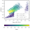 |
Fig. A.1. Distribution of ZAMS binary orbital period, p, primary mass, M1, and the final primary BH spin of systems evolving thorough the CHE channel to become merging BBHs in our fiducial model. In this sample we only include BBH systems with inspiral times less than the age of the Universe. Different markers differentiate metallicity regimes according to the legend. For visualisation purposes, we capped the color bar at aBH1 = 0.7 even though there are BHs approaching the general relativistic limit aBH1 = 1. Although binaries with p < 1 day do tidally spin up and evolve through CHE, they later undergo mass loss due to PPISN which depletes the WR star of its angular momentum reservoir. |
Appendix B: χeff − z correlation with channel exclusion
In this appendix, we show the impact to our results presented in Figure 2 in the hypothetical scenario that one of the three channels considered has a negligible contribution to the formation of merging BBHs.
First, we consider neglecting the CE channel. Factors that might lead to this hypothetical scenario are discussed in Section 4. Figure B.1 shows how the results presented in Figure 2 would change under this assumption. In this alternative model, the intrinsic fraction fχeff > 0.2(z) is mainly supported by highly spinning BBHs formed from the CHE channel at z < 5, while at larger redshift the SMT channel contributes with a larger fraction of tidally spun-up BHs. However, we notice that in contrast to our fiducial model the intrinsic fraction fχeff > 0.2(z) is monotonically decreasing. On the other hand the LIGO–Virgo detectable BBH population shows a similar behavior to the fiducial model. This is because the CE channel contribution to the LIGO–Virgo detectable population is small compared to the SMT and CHE channels, since the CE channel leads to less massive BBHs (cf. Figure 2).
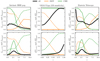 |
Fig. B.1. Fractions of BBHs with fχeff > 0.2 and fχeff > 0.5 as a function of redshift (solid lines), and the relative contribution of each field BBH channel, fchannel, according to the legend (dashed lines). The details are the same as in Figure 2, however, the model of isolated binary evolution excludes the CE channel. |
Second, we consider neglecting the SMT channel. Figure B.2 shows how the results presented in Figure 2 would change under this assumption. Because at low redshifts (z < 5) the SMT channel mostly contributes to the intrinsic distribution with non-spinning BBHs, this alternative scenario leads to a larger fχeff > 0.2(z) fraction compared to the fiducial model. This hypothetical scenario would result in a LIGO–Virgo detectable BBH population  , in tension with GWTC-3 observations.
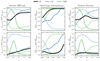 |
Fig. B.2. Fractions of BBHs with fχeff > 0.2 and fχeff > 0.5 as a function of redshift (solid lines), and the relative contribution of each field BBH channel, fchannel, according to the legend (dashed lines). The details are the same as in Figure 2, however, the model of isolated binary evolution excludes the SMT channel. |
Lastly, we consider neglecting the CHE channel. As discussed in Section 4, this might occur, for example, in the hypothetical case where the abundance of binary stars at ZAMS with short orbital periods (p < 2 days) is overestimated. This alternative model is presented in Figure B.3. We can see that the fχeff > χ0(z) distribution is similar to what is presented in Figure 2. This is explained by the fact that for any redshift the CHE channel has a small contribution to the intrinsic population of merging BBHs at fCHE(z)< 0.2. On the other hand, the LIGO–Virgo detectable  manifests an almost flat behavior up to z = 0.6 above which it sharply increases to reach unity at z ≃ 1. This sharp monotonic increase of
  is due to the contribution of tidally spun up BBHs formed from the CE channel completely dominates over BBHs formed from the SMT channel at z > 0.75, as
  .
.
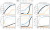 |
Fig. B.3. Fractions of BBHs with fχeff > 0.2 and fχeff > 0.5 as a function of redshift (solid lines), and the relative contribution of each field BBH channel, fchannel, according to the legend (dashed lines). The details are the same as in Figure 2, however, the model of isolated binary evolution excludes the CHE channel. |
A comparison between the intrinsic fχeff > 0.2(z) when excluding one of the three field channels and the inferred distribution given the phenomenological model presented in Eq. (4) is shown in Figure B.4. We can see that a model without the CHE channel is closer to the median inferred intrinsic fraction of fχeff > 0.2 than the fiducial model. Additionally, the model excluding the SMT channel is incompatible with the 90% CI of the inferred fraction as it overpredicts the fraction of highly rotating BBHs.
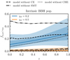 |
Fig. B.4. High-χeff fractions in the underlying distribution inferred from the population fit described in Section 3.3, in blue and orange according to the legend. The details are the same as in Figure 5, however, the models shown exclude one of the three channels according to the legend. |
All Figures
|
Fig. 1. Effective spin parameter, χeff, distribution of field BBHs as a function of redshift, z. Left: modeled intrinsic (underlying) population of field merging BBHs. Center: modeled detectable LIGO–Virgo BBH population assuming simulated O3 detector sensitivity selection effects. Right: modeled Einstein Telescope detectable BBH population assuming a forecast detector sensitivity as in Hild et al. (2011). In all cases, the fraction of non-spinning BBHs decreases as a function of redshift, shifting the χeff distribution to larger χeff values. |
| In the text | |
|
Fig. 2. Fractions of BBHs with fχeff > 0.2 and fχeff > 0.5 as a function of redshift (solid lines), and the relative contribution of each field BBH channel, fchannel, according to the legend (dashed lines). Black solid lines show the fraction of systems that satisfy a given χeff criteria for the combined CE, SMT, and CHE channels with redshift-dependent branching fractions accounted for. Left: modeled intrinsic (underlying) population of field merging BBHs. Center: modeled LIGO–Virgo detectable BBH population assuming simulated O3 detector sensitivity selection effects. Right: modeled Einstein Telescope detectable BBH population assuming forecast detector sensitivity as in Hild et al. (2011). In most cases, the fraction of highly spinning BBHs increases as a function of redshift. |
| In the text | |
|
Fig. 3. Modeled and observed fractions of BBHs satisfying |
| In the text | |
|
Fig. 4. Underlying χeff distribution from fitting the population model of Eq. (4) to the GWTC-3 BBH events. We plot the χeff population distribution at two redshift slices, z = 0 (blue) and z = 1 (orange). Solid lines denote the median and shaded bands denote the 90% CI. |
| In the text | |
|
Fig. 5. High-χeff fractions in the underlying distribution inferred from the population fit described in Sect. 3.3, in blue and orange according to the legend. Lighter contour colors indicate larger CIs of 50% and 90%, respectively. The fraction of BBH systems with large positive spins in the underlying population may increase with increasing redshift (credibility 82%), consistent with our model predictions (black). We do not yet have enough BBH events at z ∼ 1 to accurately measure the χeff distribution at high z and therefore cannot confidently conclude that the distribution is evolving. |
| In the text | |
|
Fig. 6. Redshift and effective spin parameters of the 69 confident BBH observations drawn from the GWTC-3 posteriors (orange; “observed”) compared to 69 draws from the inferred distribution fit (blue; “predicted”) described in Sect. 3.3. Each marker shape corresponds to a different set of 69 draws. We plot ten total sets. The inferred model sometimes over-predicts the largest observed χeff, while the bulk of both observed and predicted draws cover an equivalent portion of the z − χeff plane in a comparable abundance, confirming that the inferred model is a good fit for the data. |
| In the text | |
|
Fig. A.1. Distribution of ZAMS binary orbital period, p, primary mass, M1, and the final primary BH spin of systems evolving thorough the CHE channel to become merging BBHs in our fiducial model. In this sample we only include BBH systems with inspiral times less than the age of the Universe. Different markers differentiate metallicity regimes according to the legend. For visualisation purposes, we capped the color bar at aBH1 = 0.7 even though there are BHs approaching the general relativistic limit aBH1 = 1. Although binaries with p < 1 day do tidally spin up and evolve through CHE, they later undergo mass loss due to PPISN which depletes the WR star of its angular momentum reservoir. |
| In the text | |
|
Fig. B.1. Fractions of BBHs with fχeff > 0.2 and fχeff > 0.5 as a function of redshift (solid lines), and the relative contribution of each field BBH channel, fchannel, according to the legend (dashed lines). The details are the same as in Figure 2, however, the model of isolated binary evolution excludes the CE channel. |
| In the text | |
|
Fig. B.2. Fractions of BBHs with fχeff > 0.2 and fχeff > 0.5 as a function of redshift (solid lines), and the relative contribution of each field BBH channel, fchannel, according to the legend (dashed lines). The details are the same as in Figure 2, however, the model of isolated binary evolution excludes the SMT channel. |
| In the text | |
|
Fig. B.3. Fractions of BBHs with fχeff > 0.2 and fχeff > 0.5 as a function of redshift (solid lines), and the relative contribution of each field BBH channel, fchannel, according to the legend (dashed lines). The details are the same as in Figure 2, however, the model of isolated binary evolution excludes the CHE channel. |
| In the text | |
|
Fig. B.4. High-χeff fractions in the underlying distribution inferred from the population fit described in Section 3.3, in blue and orange according to the legend. The details are the same as in Figure 5, however, the models shown exclude one of the three channels according to the legend. |
| In the text | |
Current usage metrics show cumulative count of Article Views (full-text article views including HTML views, PDF and ePub downloads, according to the available data) and Abstracts Views on Vision4Press platform.
Data correspond to usage on the plateform after 2015. The current usage metrics is available 48-96 hours after online publication and is updated daily on week days.
Initial download of the metrics may take a while.