| Issue |
A&A
Volume 657, January 2022
|
|
|---|---|---|
| Article Number | A86 | |
| Number of page(s) | 9 | |
| Section | The Sun and the Heliosphere | |
| DOI | https://doi.org/10.1051/0004-6361/202141960 | |
| Published online | 18 January 2022 | |
Empirical relations between the intensities of Lyman lines of H and He+
1
Institut d’Astrophysique Spatiale, CNRS/Univ. Paris-Sud, Université Paris-Saclay, Bât. 121, 91405 Orsay, France
e-mail: This email address is being protected from spambots. You need JavaScript enabled to view it.
2
Southwest Research Institute, 1050 Walnut St., Suite 426, Boulder, CO 80302, USA
3
National Astronomical Observatory of Japan, National Institutes of Natural Sciences, 2-21-1 Osawa, Mitaka, Tokyo 181-8588, Japan
4
Institute of Space and Astronautical Science, Japan Aerospace Exploration Agency, 3-1-1 Yoshinodai, Chuo-ku, Sagamihara, Kanagawa 252-5210, Japan
5
NASA Marshall Space Flight Center, ZP 13, Huntsville, AL 35812, USA
6
Instituto de Astrofísica de Canarias, 38205 La Laguna, Tenerife, Spain
Received:
5
August
2021
Accepted:
28
September
2021
Abstract
Context. Empirical relations between major UV and extreme UV spectral lines are one of the inputs for models of chromospheric and coronal spectral radiances and irradiances. They are also needed for the interpretation of some of the observations of the Solar Orbiter mission.
Aims. We aim to determine an empirical relation between the intensities of the H I 121.6 nm and He II 30.4 nm Ly-α lines.
Methods. Images at 121.6 nm from the Chromospheric Lyman-Alpha Spectro Polarimeter (CLASP) and Multiple XUV Imager (MXUVI) sounding rockets were co-registered with simultaneous images at 30.4 nm from the EIT and AIA orbital telescopes in order to derive a spatially resolved relationship between the intensities.
Results. We have obtained a relationship between the H I 121.6 nm and He II 30.4 nm intensities that is valid for a wide range of solar features, intensities, and activity levels. Additional SUMER data have allowed the derivation of another relation between the H I 102.5 nm (Ly-β) and He II 30.4 nm lines for quiet-Sun regions. We combined these two relationships to obtain a Ly-α/Ly-β intensity ratio that is comparable to the few previously published results.
Conclusions. The relationship between the H I 121.6 nm and He II 30.4 nm lines is consistent with the one previously obtained using irradiance data. We have also observed that this relation is stable in time but that its accuracy depends on the spatial resolution of the observations. The derived Ly-α/Ly-β intensity ratio is also compatible with previous results.
Key words: Sun: chromosphere / Sun: UV radiation
© M. Gordino et al. 2022
 Open Access article, published by EDP Sciences, under the terms of the Creative Commons Attribution License (https://creativecommons.org/licenses/by/4.0), which permits unrestricted use, distribution, and reproduction in any medium, provided the original work is properly cited.
1. Motivation
The Ly-α and Ly-β lines of neutral hydrogen respectively at 121.6 nm and 102.5 nm and the Ly-α line of singly ionized helium at 30.4 nm are among the brightest lines of the ultraviolet (UV) spectrum of the Sun, and their study is of importance in many areas of solar physics. These lines are observed by several instruments on board the Solar Orbiter mission (Müller et al. 2020). In this paper, we derive empirical relationships between these lines with, as described below, three main applications in mind: (i) the modeling of the resonance scattering emission of these lines in the corona, taking the nonuniformity of the chromospheric source into account, (ii) the observational constraint of nonlocal thermodynamic equilibrium (NLTE) models of chromospheric structures, and (iii) the modeling of the UV and extreme UV (EUV) irradiances.
The bright coronal Ly-α line is mainly formed by the resonant scattering of the underlying chromospheric radiation by residual neutral hydrogen (Gabriel 1971). The efficiency of the resonant scattering process depends on how much the chromospheric source profile and coronal scattering profile overlap. In a static atmosphere, the central wavelength of these two profiles lines up perfectly, whereas in a region with solar wind flow the scattering profile is Doppler-shifted relative to the disk profile, which results in a less efficient scattering and, therefore, in a reduced (dimmed) line intensity. Doppler dimming observations at Ly-α and in other lines that have a significant resonantly scattered component, such as the O VI doublet at 103.2 and 103.7 nm., have been extensively used to estimate the outflow velocities of the coronal plasma (e.g., Kohl et al. 1997; Antonucci et al. 2000). The interpretation of the Ly-α resonance scattering measurements relies on iterative forward modeling and thus requires independent knowledge of the chromospheric intensity, which is often taken from in-ecliptic irradiance measurements. However, Auchère (2005) has shown that using disk-integrated values and thus not taking into account the anisotropy of the illumination of the corona resulting from the distribution of bright features (e.g., active regions) and dark features (e.g., coronal holes) in the chromosphere can lead to significant systematic over- or underestimations of the coronal intensity, especially in polar regions. Recently, Dolei et al. (2018, 2019) estimated that this translates to a 50 km s−1 error on the outflow velocities derived from Doppler dimming methods. The same effect applies to all resonantly scattered coronal lines (i.e., the Ly-α line of He II at 30.378 nm). Calibrated Ly-α disk images are thus in principle necessary for interpreting the coronal observations1. While 30.4 nm disk images are routinely available from narrowband telescopes such as the Extreme-ultraviolet Imaging Telescope (EIT; Delaboudinière et al. 1995), the Extreme Ultra Violet Imager (EUVI; Wuelser et al. 2004), or the Atmospheric Imaging Assembly (AIA; Boerner et al. 2012; Lemen et al. 2012), full-disk Ly-α observations are rare (e.g., Bonnet et al. 1980). Auchère (2005) thus introduced the possibility of using scaled 30.4 nm images as proxies for Ly-α data, which requires the derivation of an empirical relationship between the intensities of the two lines.
The chromospheric Ly-α line of hydrogen was first observed by Purcell & Tousey (1960) in a 1959 rocket flight and since then has been the subject of many more observations (see below), along with theoretical and modeling works. However, the profile of the line (very often self-reversed) has led to questions concerning both its characterization and interpretation. The line is optically thick and formed in non-local thermodynamic equilibrium (NLTE; Jefferies & Thomas 1961; Morton & Widing 1961), a situation that complicates the spectroscopic diagnostic. Nonetheless, the comparison of model outputs and observed line profiles of Ly-α, Ly-β (which is also self-reversed; Tousey 1963), and other strong UV lines was at the root of one-dimensional (1D) models such as the Vernazza, Avrett, Loeser (VAL; Vernazza et al. 1981) and later the Fontenla, Avrett, Loeser (FAL; Fontenla et al. 1990) models. Observations from the Orbiting Solar Observatory 8 (OSO 8) spacecraft and from sounding rockets (Bonnet et al. 1978, 1982; Gouttebroze et al. 1978; Bonnet 1981) of the Ly-α and Ly-β lines have led to the modeling of the chromosphere, active regions (e.g., Lemaire et al. 1981), sunspots (Kneer et al. 1981; Lites & Skumanich 1982), and prominences (Vial 1982). In our present theoretical effort, the Ly-β line was also used because it was simultaneously observed with the Ly-α line and provided a complementary diagnostic.
H0 and He+ have similar atomic structures, and NLTE modeling has shown that their Ly-α photons come from close-by but different layers of the solar atmosphere, although the details of the processes themselves may differ from one line to the other. Ly-α and Ly-β lines of H I are thermally produced (electronic collisions) in the chromosphere up to 30 000 K, and the Ly-α of He II is formed above 30 000 K. On the contrary, in prominences, the Ly-α photons are mainly radiatively produced by resonance scattering. Radiation also plays an important role in the formation of the line of He II since the existence of the He+ ion is determined by the incident EUV coronal radiation (e.g., Andretta et al. 2003). Moreover, the three lines play a very important role in the radiative losses of the various solar features (see the VAL and FAL models for the chromosphere or the case of radiative equilibrium for prominences in Heinzel & Anzer 2012). This means that simultaneous observations of the three abovementioned lines are (or would be) very useful for modeling the various solar structures. Despite the difficulties in recording the Ly-α line, nearly simultaneous observations of the Ly-α and Ly-β lines of H I were possible with the Solar Ultraviolet Measurement of Emitted Radiation (SUMER; Wilhelm et al. 1995) spectrograph, and Lemaire et al. (2012) were able to constrain the ratio between the intensities of the two lines in various solar structures. A correlation between the intensities of the Ly-α lines of H I and He II has been obtained by Auchère (2005), but, to the best of our knowledge, no relation has yet been established between the Ly-β line of H I and the Ly-α line of He II.
Irradiance modeling is closely related to the two previous objectives. Semiempirical models of the solar spectral radiance adjust the variation in temperature with height in the solar atmosphere to obtain optimum agreement between calculated and observed continuum intensities, line intensities, and line profiles (Avrett & Loeser 2008). Major constraints to these models come from the observed intensities and profiles of the Ly-α and Ly-β lines (and other strong UV lines) and in fact led to the development of the seminal 1D VAL and FAL models. For instance, the observations of the self-reversal of the Ly-β line (Tousey 1963) constrained the models with the existence of a temperature plateau around 20 000 K. Using this approach, the reconstruction of the spectral irradiance is obtained by a linear combination of a family of models in which the physical parameters are adjusted to match observations for a number of solar structures: coronal holes, quiet Sun, plage, sunspot umbra, penumbra, etc. It is thus necessary to use not only irradiance values, but also resolved measurements of the lines intensities.
In Sect. 2 of the paper, we derive a new relationship between the intensities of the Ly-α lines of H I and He II using two different sets of spatially resolved data. In Sect. 3 we derive a relationship between the intensities of the Ly-β line of H I and the Ly-α line of He II. In Sect. 4 we derive a relationship between the intensities of the Ly-β and Ly-α lines of H I. We summarize our findings in Sect. 5.
2. H I 121.6 nm versus He II 30.4 nm
Auchère (2005) derived an empirical relation between the H I 121.6 nm and He II 30.4 nm irradiances using data from the EIT telescope, the Solar Stellar Irradiance Comparison Experiment (SOLSTICE; Rottman et al. 1993), and the Solar EUV Experiment (SEE; Woods et al. 2000). It matched spatially resolved but episodic observations from Skylab (Vernazza & Reeves 1978). In the present study, we revisit this relationship using two new sets of spatially resolved observations that cover all types of solar structures and different activity levels. The first set is full-disk observations made on November 2, 1998, by EIT and the Multiple XUV Imager (MXUVI; Auchère et al. 1999). The second set corresponds to disk-center and limb observations made on September 3, 2015, by the AIA and the Chromospheric Lyman-Alpha Spectro Polarimeter (CLASP; Kano et al. 2012, 2017; Kobayashi et al. 2012).
2.1. MXUVI and EIT data
The second flight of the MXUVI sounding-rocket-borne telescope occurred on November 2, 1998, at 18:20 UT. The Ly-α channel of the MXUVI uses a 256 × 256 detector with a 10 arcsec/pixel sampling. Isolation of the Ly-α line is obtained using Al/MgF2 filters and selective mirror coating for a resulting passband of 10 nm. All the data acquired during the flight were co-registered and added into a single image. The flat field and dark level were corrected according to Auchère et al. (1999). Radiometric calibration was obtained by scaling the resulting image to the simultaneous composite Ly-α irradiance, which for this date includes data from SOLSTICE (Rottman et al. 1993; Woods et al. 1993). The composite passband has a width of 1.0 nm.
The EIT telescope has been providing Sun full-disk observations since 1996. We used the November 2, 1998, image taken at 18:26 UT, which is the 30.4 nm image closest in time to the MXUVI second flight and corresponds to a specific EIT campaign for this flight. The 30.4 nm channel uses a 1024 × 1024 detector with a 2.627 arcsec pixel−1 sampling (Auchère et al. 2000; Auchère & Artzner 2004). The flat field, dark noise, and degradation were corrected with the eit_prep procedure. Radiometric calibration was obtained by using the eit_parms function. The instrument passband has a width of 7.3 nm.
2.2. CLASP and AIA data
The first flight of the CLASP sounding-rocket-borne spectro-polarimeter occurred on September 3, 2015, between 17:03 UT and 17:08 UT. The Ly-α images used are provided by the CLASP Slit-Jaw camera (CLASP-SJ). The CLASP-SJ uses a 528 × 536 pixel sensor with a 1.03 arcsec pixel−1 sampling. The instrument passband has a width of 3.5 nm. The flat field and dark level were corrected. The radiometric calibration was obtained by scaling the resulting image to the simultaneous composite Ly-α irradiance, which for this date includes data from SOLSTICE (McClintock et al. 2005a,b; Snow et al. 2005). The composite passband has a width of 1.0 nm. During this flight, images from the Sun center and limb were taken.
The AIA telescope has been providing full-disk observations at high resolution since 2010. The 30.4 nm channel of AIA uses a 4096 × 4096 detector with a 0.63 arcsec pixel−1 sampling. The 12-s cadence permitted 25 AIA images to be obtained during the CLASP flight. The radiometric calibration was obtained by using the aia_get_response function. The instrument passband has a width of 4.5 nm.
2.3. Data co-registration
We co-aligned the He II 30.4 nm (EIT or AIA) and H I 121.6 nm (MXUVI or CLASP-SJ) images to compare and find a relation between the intensities. We used a reduced χ2 cross-correlation method in translation and rotation. The spatial scaling was assumed to be known from the independently derived plate scales and from the distances between the instruments and the Sun. When scanning the parameter space, the highest resolution images (EIT and AIA) were resampled using bilinear interpolation in the reference frame of the lowest resolution images (MXUVI and CLASP), the latter being left untouched. For CLASP-SJ, each image was co-registered with the AIA image that was closest in time. We validated our procedure by co-aligning an EIT 30.4 nm image with an AIA 30.4 nm image taken on August 1, 2011, at 01:07 UT. Since the pointing information of the two instruments is known independently from the headers of the images, this test shows that the co-alignment error is about 0.15 pixels rms. This translates to 0.16 arcsec for AIA-CLASP pairs and 1.6 arcsec for EIT-MXUVI pairs. These sub-pixel co-alignment errors contribute negligible dispersion to the correlations described in Sect. 2.5. Figure 1 shows the H I 121.6 nm MXUVI and the He II 30.4 nm EIT images after co-registration. The first two images were used to find the relationship between the intensities of the two lines and correspond to MXUVI and EIT images with a 10 arcsec pixel resolution. In the third image, which shows the original full resolution EIT data, colored contours correspond to different solar regions. Figures 2 and 3 show the H I 121.6 nm CLASP-SJ and the He II 30.4 nm AIA images after co-registration for, respectively, Sun center and limb observations.
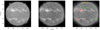 |
Fig. 1. Quasi-simultaneous images of the Sun taken on November 2, 1998, in H I 121.6 nm (left) and He II 30.4 nm (center, right). The Lyman-α image was obtained by the rocket-borne MXUVI instrument at 18:20 UT. The 30.4 nm image was recorded by EIT at 18:26 UT. The EIT image was degraded to match the resolution of the MXUVI. Solar north is up. The intensity scales are logarithmic in both cases, and the contrast is the same. There is a remarkable morphological similarity for all types of structures, but, as is also visible in Fig. 4, they are less contrasted at Lyman α. In the right image, we overlaid different contours corresponding to different solar regions: active regions (red), filaments (green), the coronal hole (yellow), and prominences (purple). |
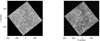 |
Fig. 2. Sun center H I 121.6 nm observations from September 3, 2015, from the CLASP-SJ (left) and simultaneous He II 30.4 nm observations from AIA degraded to match the CLASP-SJ resolution (right). The black band in the center of the CLASP-SJ image is the entrance slit of the spectrometer. Solar north is up. |
2.4. Isolation of the HeII 30.4 nm line
In addition to the main line of He II at 30.378 nm, the 30.4 nm passbands of EIT and AIA include several coronal and transition region lines. In particular, the Si XI line at 30.332 nm cannot be suppressed by the multilayer coating technology of these instruments. In order to estimate the contribution of all the contaminating spectral lines from the EIT and AIA, we constructed a differential emission measure (DEM) curve for each pixel of the images. Then, knowing the spectral response of the instruments, we computed the intensity of all the spectral lines included in the passbands except for that of He II at 30.378 nm. The sum of their contributions was then removed from the original 30.4 nm image to obtain the intensity of the He II 30.378 nm line alone. For EIT, the DEM curve was constructed using the code developed specifically for EIT by Cook et al. (1999) and used in Auchère et al. (2005a) to compute the He II irradiance. For AIA, we used the Gaussian DEM inversion from Guennou et al. (2012a,b). As a validation, we verified that the computed intensity of the Si XI line represents 5 to 20% of that of the He II line, in agreement with the spectroscopically derived values of Thompson & Brekke (2000).
2.5. Results
In Fig. 4 we have represented the intensity of the H I 121.6 nm line measured by MXUVI as a function of that of the He II line at 30.4 nm measured by EIT. We fitted the data points with the following function:
![Mathematical equation: $$ \begin{aligned} I_{121.6} = C_{1}(1-C_{2}e^{-C_{3}I_{30.4}}) \ [\mathrm{W} .\mathrm{m} ^{-2}.\mathrm{sr} ^{-1}] .\end{aligned} $$](/articles/aa/full_html/2022/01/aa41960-21/aa41960-21-eq1.gif) (1)
(1)
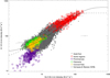 |
Fig. 4. Correlation between He II 30.4 nm and H I 121.6 nm for the November 2, 1998, data set (MXUVI and EIT). The cross on the right indicates the error bars for each data point. The different colored circles on the plot correspond to the intensities of the colored contours in the EIT image (Fig. 1). The dark squares are the Vernazza & Reeves (1978) data from Skylab, shown with their error bars. The solid line fits the MXUVI and EIT data. The dashed line corresponds to the fit from Auchère (2005). |
This relation was introduced by Vourlidas et al. (2001), and it was used by Auchère (2005) to fit the correlation between the H I 121.6 nm and He II 30.4 nm irradiances. The best-fit parameters are given in Table 1 along with those obtained by Auchère (2005). The solid and dashed curves in Fig. 4 correspond respectively to the present fit and to that of Auchère (2005). The colored circles correspond to the contribution of the different solar regions encircled in the third image of Fig. 1. As observed by Auchère (2005), we notice in active regions (red circles) a saturation effect at high intensities. The prominence data points have a distinct distribution because of the predominantly radiative formation process of that line compared to other types of structures. It should be noted that the data points corresponding to prominences were not taken into account for the fit. Indeed, for the primary application of coronal modeling, prominences represent a negligible contribution. The uncertainty for EIT intensities is about 25%, and the uncertainty for the Ly-α irradiance from SOLSTICE is about 5% for November 2, 1998 (Snow, priv. commun.). The offset between the two fits, at most 30%, can thus be explained by calibration uncertainties. We also plot the data from Skylab (Vernazza & Reeves 1978) (squares), which match with the two relations found. This shows that the correlation between He II 30.4 nm intensity and H I 121.6 nm intensity is stable with time.
Comparison between the fitted coefficients of Eq. (1) for the data sets considered in the present work and those in Auchère (2005).
Figure 5 shows the intensity of CLASP-SJ H I 121.6 nm as a function of AIA He II 30.4 nm intensity. The uncertainties for AIA 30.4 nm are about 25% (Boerner et al. 2012). Regarding the Ly-α irradiance from SOLSTICE, the uncertainties are about 8% for September 3, 2015 (Snow, priv. comm.). The two panels correspond to two spatial resolutions: the CLASP-SJ resolution (1.03 arcsec, left) and binned to the MXUVI resolution (10 arcsec, right). The solid lines in the two plots correspond to the relation derived in the previous section from MXUVI and EIT data. The dotted-dashed line corresponds to the relation derived from CLASP and AIA images, and the dashed line corresponds to the relation derived from both data sets. These fits have been calculated with images at the MXUVI resolution. The colored contours correspond to the clusters of colored circles in Fig. 4. They show that the relations we obtained from CLASP-SJ and AIA images can also describe the correlation between the H I 121.6 nm and He II 30.4 nm lines from MXUVI-EIT images. This confirms, as mentioned above, that the relation between He II 30.4 nm and H I 121.6 nm intensities is stable in time.
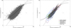 |
Fig. 5. Correlation between He II 30.4 nm and H I 121.6 nm for the September 3, 2015, data set (CLASP-SJ and AIA). The plot in the left panel corresponds to the 1.03 arcsec pixel−1 CLASP-SJ resolution, whereas the plot in the right panel has the 10 arcsec pixel−1 MXUVI resolution. The cross on the right of each plot indicates the error bars for each data point. The solid lines correspond to the fit shown in Fig. 4. The dot-dashed lines correspond to the fit of the CLASP (at MXUVI resolution) and AIA data. The dashed lines show the fit for both the MXUVI-EIT and CLASP-AIA data. The colored contours outline the intensity distributions for the different solar regions from Fig. 4. |
The best-fit relationships of Figs. 4 and 5 are consistent given the uncertainties of each data set. While being thus equivalent, the corresponding uncertainties must be propagated when being used for the possible applications listed in Sect. 1. We also notice that there is more dispersion in the left plot of Fig. 5, which corresponds to the higher resolution images. It shows that the correlation is stronger when one observes at lower spatial resolution. This is consistent with the extreme case of the disk-integrated data used by Auchère (2005), for which the dispersion was even smaller. Consequently, the empirical relationships given here are particularly suited for applications that do not require high spatial resolution, such as the coronal and irradiance modeling described in Sect. 1. The increase in dispersion with increased resolution is possibly a signature of the differences between the formation processes of the two lines. We also notice that the dispersion is larger in He II than in H I. This could be explained by the sensitivity of the Planckian (collisional) contribution to the source function, since its sensitivity to temperature is proportional to the frequency. There is also a clearly different behavior between the quiet Sun and prominences for a given He II intensity (see Fig. 4). The study of these differences is potentially important for chromospheric modeling but is beyond the scope of this paper.
3. H I 102.5 nm versus He II 30.4 nm
3.1. SUMER and EIT data
In order to derive this relationship, we used data from the SUMER instrument. We used a Ly-β line raster measured on April 8, 1996, between 06:09 UT and 06:36 UT, close to the Sun center. The spectra we used were recorded by the SUMER/A detector, which has 1024 (spectral) × 360 (spatial) pixels2. The slit used for the raster was the 1 × 120 arcsec2 one. The raster contains 313 spectra at the Ly-β line with a step of 0.38 arcsec between each spectrum. Each spectrum covers a 0.7 nm width. We used the standard preparation routine, sum_read_corr_fits, which includes the radiometric calibration. For the 30.4 nm data, we used the April 8, 1996, EIT image taken at 06:21 UT, which is the image closest in time to the SUMER raster.
3.2. Data processing
In order to build the SUMER raster image, we integrated the intensity along the wavelength axis to obtain the total intensity at each point of the field of view. We then degraded the resulting SUMER image by smoothing it down to the EIT 2.627 arcsec resolution. We used the same co-alignment procedure used for the study of the correlation between He II 30.4 nm and H I 121.6 nm intensities (Sect. 2.3). Figure 6 shows the resulting H I 102.5 nm SUMER image (left) along with the co-registered EIT image (middle). These two images were used to find the relationship between the two lines. The third image (right) shows the original EIT data, the white square indicating the region covered by the SUMER raster.
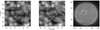 |
Fig. 6. Observations from SUMER at the H I Lyman-β line on April 8, 1996, at 06:09:27 UT (left) and EIT at the He II 30.4 nm line on April 8, 1996, at 06:21:51 UT, corresponding to the SUMER field of view (middle) and the full-disk observation (right). The white square on the full-disk EIT image shows the position of the SUMER field of view. |
3.3. Results
Figure 7 shows the SUMER H I 102.5 nm intensity as a function of the EIT He II 30.4 nm intensity. The solid curve corresponds to a linear fit to the data with the following relation:
![Mathematical equation: $$ \begin{aligned} I_{102.5} = 0.132 I_{30.4} + 0.0233 \ [\mathrm{W} \,\mathrm{m} ^{-2}\,\mathrm{sr} ^{-1}] .\end{aligned} $$](/articles/aa/full_html/2022/01/aa41960-21/aa41960-21-eq2.gif) (2)
(2)
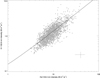 |
Fig. 7. Correlation between He II 30.4 nm from EIT and H I 102.5 nm from SUMER. The cross at the bottom right indicates the error bars for each data point. The solid line is an estimation of the correlation with a linear fit. |
The uncertainties for SUMER intensities are about 20%. Eq. (2) was obtained using only quiet-Sun data, covering a limited range of intensities, which justifies the linear fit. We note that the ratio I30.4/I102.5 is about 8 in the quiet Sun, to be compared to the irradiance ratio (in the range 5–10, e.g., in June 2010; SEE 2016), the Vernazza & Reeves (1978) ratio of 11, or the X-flare ratio (about 5; Milligan et al. 2012).
4. H I 102.5 nm versus H I 121.6 nm
Lemaire et al. (2012) measured the Ly-α/Ly-β ratio from SUMER data, which were obtained in coronal holes, the quiet Sun, and active regions. As we have two relationships, between He II and H I Ly-α and between He II and H I Ly-β, we can indirectly obtain a relationship between H I Ly-α and H I Ly-β. In order to do this, we used the November 2, 1998, EIT 30.4 nm image converted to Ly-β using Eq. (2). This requires the assumption that Eq. (2), which was derived for April 8, 1996, still holds for November 2, 1998. We also suppose that Eq. (2), obtained for the quiet Sun, can be extrapolated to regions of higher intensities. In order to compare our results to the ones of Lemaire et al. (2012), we plot in Fig. 8 the Ly-α/Ly-β intensity ratio as a function of the Ly-α intensity. We chose a range that matches the range of validity of Eq. (2). Using Eqs. (1) and (2), we can derive a relation for the Ly-α/Ly-β intensity ratio. This relation is represented in Fig. 8 by the three-dotted-dashed line. As in Sect. 2, prominences are not taken into consideration to derive Eq. (1). We trace the three fits from Lemaire et al. (2012), which correspond to one coronal hole and two quiet-Sun observations. We notice higher ratios for coronal holes and lower ratios for active regions than for the quiet Sun. We also plot values that can be derived from the intensities obtained by Patsourakos et al. (1998) from OSO 8 spectra. These values are represented by the large circles and correspond respectively to, from left to right, cell, network, bright point, and plage. This shows that our Ly-α/Ly-β ratio is in the range of values measured by Lemaire et al. (2012) and deduced from Patsourakos et al. (1998). However, they do not agree with the higher values derived by Tian et al. (2009a) and Tian et al. (2009b) for the quiet Sun (about 200) and a coronal hole (130). An explanation of these discrepancies is given in Lemaire et al. (2012). Given the uncertainties of about 50% on the Ly-α/Ly-β ratio, represented by the stars with error bars, our values for coronal holes are compatible with those of Lemaire et al. (2012). However, as pointed out by Bocchialini & Vial (1994, 1996) and Patsourakos et al. (1997), the Ly-α and Ly-β lines appear to have a singular behavior in equatorial coronal holes. For active regions, the ratio is lower. This can be explained if the linear relationship between H I 102.5 nm and He II 30.4 nm is not valid for active regions. To be fully compatible with Lemaire et al. (2012), including for active regions, we can predict that the relationship between He II 30.4 nm and H I 102.5 nm in fact saturates at high intensities, such as the one found between He II 30.4 nm and H I 121.6 nm (Sect. 2). We note that the Ly-α/Ly-β ratio is much higher (210) in a streamer at about 1 R⊙ above the surface (Giordano et al. 2013). Such a high value could be explained by the importance of resonance scattering in both lines. We finally mention that in the case of a coronal mass ejection (CME) found a ratio of about 4, while Ciaravella et al. (2003) report a ratio of 450 in the pre-CME and CME phases.
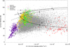 |
Fig. 8. Distribution of the H I Ly-α/Ly-β intensity ratio from the MXUVI image and the EIT image converted to Ly-β using Eq. (2). The dots and colored circles represent the measurements, which were performed at a period of minimum activity. The colored circles correspond to the different solar regions defined in Fig. 4. In order to maintain SI units, Ly-α intensities are expressed in mW m−2 sr−1, providing numerical values equivalent to the centimeter-gram-second units of erg s−1 cm−2 sr−1 used by Lemaire et al. (2012). The three-dotted-dashed line represents the H I Ly-α/Ly-β intensity ratio deduced from Eqs. (1) and (2). The stars with error bars give an estimate of the accuracy of the ratio. The three other lines are the fits from Fig. 2 of Lemaire et al. (2012). The solid and dashed lines correspond to two quiet-Sun observations, whereas the dotted-dashed line corresponds to a coronal hole. The squares with error bars on these lines give an estimation of the error for different ratio values on the three fits. The large black circles correspond to the ratio deduced from Patsourakos et al. (1998). |
5. Conclusions
Using full-disk images, we derived an empirical relationship between H I Ly-α and He II 30.4 nm intensities. Considering the uncertainties and the scatter on the intensities, our results are compatible with those obtained by Auchère (2005) from irradiance measurements, as well as with the spatially resolved results of Vernazza & Reeves (1978). As the observations span four decades and various levels of activity, we conclude that this relationship is stable in time. We also observed that the dispersion around the average relationship increases with increasing resolution, which could have implications for NLTE modeling. We derived a new relation between the H I Ly-β and He II 30.4 nm intensities for two quiet-Sun regions. Combined with the H I Ly-α and He II 30.4 nm relationship, we also obtained a Ly-α/Ly-β intensity ratio compatible with previous results in the quiet Sun, which can be used to constrain chromospheric emission models. Our results are not only important for the modeling of various solar features, but also for the reconstruction of the spectral irradiance in H I and He II lines, which are important radiative input components in the Earth’s ionosphere and thermosphere.
The three lines studied in this paper can be observed simultaneously by the Extreme Ultraviolet Imager (EUI; Halain et al. 2015; Rochus et al. 2020) telescope, the Spectral Imaging of the Coronal Environment (SPICE; Spice Consortium 2020) spectrometer, and the Metis (Antonucci et al. 2012, 2020) coronagraph on Solar Orbiter (Müller & St. Cyr 2013; Müller et al. 2020). The derived relationships will help in the joint analysis of the observations of these three instruments (Auchère et al. 2020). In particular, the relationships derived in this paper are needed to analyze the Metis observations of the resonantly scattered emission of H I in the corona. Since Metis does not measure the Ly-α disk intensity, it is possible to instead use 30.4 nm data from the full-Sun channel of the EUI telescope (Auchère et al. 2005b) to compute the illumination of the corona at 121.6 nm.
This is also true of the modeling of the Ly-α radiation back-scattered by interplanetary neutral hydrogen (Cook et al. 1981).
References
- Andretta, V., Del Zanna, G., & Jordan, S. D. 2003, A&A, 400, 737 [NASA ADS] [CrossRef] [EDP Sciences] [Google Scholar]
- Antonucci, E., Dodero, M. A., & Giordano, S. 2000, Sol. Phys., 197, 115 [NASA ADS] [CrossRef] [Google Scholar]
- Antonucci, E., Fineschi, S., Naletto, G., et al. 2012, in Space Telescopes and Instrumentation 2012: Ultraviolet to Gamma Ray, Proc. SPIE, 8443, 844309 [NASA ADS] [CrossRef] [Google Scholar]
- Antonucci, E., Romoli, M., Andretta, V., et al. 2020, A&A, 642, A10 [NASA ADS] [CrossRef] [EDP Sciences] [Google Scholar]
- Auchère, F. 2005, ApJ, 622, 737 [Google Scholar]
- Auchère, F., & Artzner, G. E. 2004, Sol. Phys., 219, 217 [CrossRef] [Google Scholar]
- Auchère, F., Hassler, D. M., Slater, D. C., & Woods, T. N. 1999, in EUV, X-Ray, and Gamma-Ray Instrumentation for Astronomy X, eds. O. H. Siegmund, & K. A. Flanagan, Proc. SPIE, 3765, 351 [CrossRef] [Google Scholar]
- Auchère, F., DeForest, C. E., & Artzner, G. 2000, ApJ, 529, L115 [CrossRef] [Google Scholar]
- Auchère, F., Cook, J. W., Newmark, J. S., et al. 2005a, ApJ, 625, 1036 [CrossRef] [Google Scholar]
- Auchère, F., Song, X., Rouesnel, F., et al. 2005b, in Solar Physics and Space Weather Instrumentation, eds. S. Fineschi, & R. A. Viereck, Proc. SPIE, 5901, 298 [Google Scholar]
- Auchère, F., Andretta, V., Antonucci, E., et al. 2020, A&A, 642, A6 [NASA ADS] [CrossRef] [EDP Sciences] [Google Scholar]
- Avrett, E. H., & Loeser, R. 2008, ApJS, 175, 229 [Google Scholar]
- Bocchialini, K., & Vial, J.-C. 1994, A&A, 287, 233 [NASA ADS] [Google Scholar]
- Bocchialini, K., & Vial, J.-C. 1996, Sol. Phys., 168, 37 [NASA ADS] [CrossRef] [Google Scholar]
- Boerner, P., Edwards, C., Lemen, J., et al. 2012, Sol. Phys., 275, 41 [Google Scholar]
- Bonnet, R. M. 1981, Space Sci. Rev., 29, 131 [NASA ADS] [CrossRef] [Google Scholar]
- Bonnet, R. M., Lemaire, P., Vial, J. C., et al. 1978, ApJ, 221, 1032 [NASA ADS] [CrossRef] [Google Scholar]
- Bonnet, R. M., Decaudin, M., Bruner, E. C., Jr, Acton, L. W., & Brown, W. A. 1980, ApJ, 237, L47 [NASA ADS] [CrossRef] [Google Scholar]
- Bonnet, R. M., Decaudin, M., Foing, B., et al. 1982, A&A, 111, 125 [NASA ADS] [Google Scholar]
- Ciaravella, A., Raymond, J. C., van Ballegooijen, A., et al. 2003, ApJ, 597, 1118 [NASA ADS] [CrossRef] [Google Scholar]
- Cook, J. W., Meier, R. R., Brueckner, G. E., & van Hoosier, M. E. 1981, A&A, 97, 394 [NASA ADS] [Google Scholar]
- Cook, J. W., Newmark, J. S., & Moses, J. D. 1999, in 8th SOHO Workshop: Plasma Dynamics and Diagnostics in the Solar Transition Region and Corona, eds. J. C. Vial, & B. Kaldeich-Schü, ESA SP, 446, 241 [Google Scholar]
- Delaboudinière, J.-P., Artzner, G. E., Brunaud, J., et al. 1995, Sol. Phys., 162, 291 [CrossRef] [Google Scholar]
- Dolei, S., Susino, R., Sasso, C., et al. 2018, A&A, 612, A84 [NASA ADS] [CrossRef] [EDP Sciences] [Google Scholar]
- Dolei, S., Spadaro, D., Ventura, R., et al. 2019, A&A, 627, A18 [NASA ADS] [CrossRef] [EDP Sciences] [Google Scholar]
- Fontenla, J. M., Avrett, E. H., & Loeser, R. 1990, ApJ, 355, 700 [NASA ADS] [CrossRef] [Google Scholar]
- Gabriel, A. H. 1971, Sol. Phys., 21, 392 [Google Scholar]
- Giordano, S., Ciaravella, A., Raymond, J. C., Ko, Y.-K., & Suleiman, R. 2013, J. Geophys. Res. (Space Phys.), 118, 967 [NASA ADS] [CrossRef] [Google Scholar]
- Gouttebroze, P., Lemaire, P., Vial, J. C., & Artzner, G. 1978, ApJ, 225, 655 [NASA ADS] [CrossRef] [Google Scholar]
- Guennou, C., Auchère, F., Soubrié, E., et al. 2012a, ApJS, 203, 25 [NASA ADS] [CrossRef] [Google Scholar]
- Guennou, C., Auchère, F., Soubrié, E., et al. 2012b, ApJS, 203, 26 [Google Scholar]
- Halain, J. P., Mazzoli, A., Meining, S., et al. 2015, in Solar Physics and Space Weather Instrumentation VI, Proc. SPIE, 9604, 96040H [NASA ADS] [CrossRef] [Google Scholar]
- Heinzel, P., & Anzer, U. 2012, A&A, 539, A49 [NASA ADS] [CrossRef] [EDP Sciences] [Google Scholar]
- Jefferies, J. T., & Thomas, R. N. 1961, ApJ, 133, 606 [NASA ADS] [CrossRef] [Google Scholar]
- Kano, R., Bando, T., Narukage, N., et al. 2012, in Space Telescopes and Instrumentation 2012: Ultraviolet to Gamma Ray, Proc. SPIE, 8443, 84434F [CrossRef] [Google Scholar]
- Kano, R., Trujillo Bueno, J., Winebarger, A., et al. 2017, ApJ, 839, L10 [NASA ADS] [CrossRef] [Google Scholar]
- Kneer, F., Mattig, W., Scharmer, G., et al. 1981, Sol. Phys., 69, 289 [NASA ADS] [CrossRef] [Google Scholar]
- Kobayashi, K., Kano, R., Trujillo-Bueno, J., et al. 2012, in Fifth Hinode Science Meeting, eds. L. Golub, I. De Moortel, & T. Shimizu, ASP Conf. Ser., 456, 233 [NASA ADS] [Google Scholar]
- Kohl, J. L., Noci, G., Antonucci, E., et al. 1997, Sol. Phys., 175, 613 [Google Scholar]
- Lemaire, P., Gouttebroze, P., Vial, J. C., & Artzner, G. E. 1981, A&A, 103, 160 [NASA ADS] [Google Scholar]
- Lemaire, P., Vial, J.-C., Curdt, W., Schühle, U., & Woods, T. N. 2012, A&A, 542, L25 [NASA ADS] [CrossRef] [EDP Sciences] [Google Scholar]
- Lemen, J. R., Title, A. M., Akin, D. J., et al. 2012, Sol. Phys., 275, 17 [Google Scholar]
- Lites, B. W., & Skumanich, A. 1982, ApJS, 49, 293 [NASA ADS] [CrossRef] [Google Scholar]
- McClintock, W. E., Rottman, G. J., & Woods, T. N. 2005a, Sol. Phys., 230, 225 [NASA ADS] [CrossRef] [Google Scholar]
- McClintock, W. E., Rottman, G. J., & Woods, T. N. 2005b, Sol. Phys., 230, 225 [NASA ADS] [CrossRef] [Google Scholar]
- Milligan, R. O., Chamberlin, P. C., Hudson, H. S., et al. 2012, ApJ, 748, L14 [NASA ADS] [CrossRef] [Google Scholar]
- Morton, D. C., & Widing, K. G. 1961, ApJ, 133, 596 [NASA ADS] [CrossRef] [Google Scholar]
- Müller, D., & St. Cyr, O. C. 2013, in Solar Physics and Space Weather Instrumentation V, Proc. SPIE, 8862, 88620E [CrossRef] [Google Scholar]
- Müller, D., St. Cyr, O. C., Zouganelis, I., et al. 2020, A&A, 642, A1 [Google Scholar]
- Patsourakos, S., Bocchialini, K., & Vial, J. C. 1997, in Fifth SOHO Workshop: The Corona and Solar Wind Near Minimum Activity, ed. A. Wilson, ESA Spec. Publ., 404, 577 [NASA ADS] [Google Scholar]
- Patsourakos, S., Bocchialini, K., & Vial, J. C. 1998, Acad. Sci. Paris C. R. Ser. B Sci. Phys., 326, 337 [Google Scholar]
- Purcell, J. D., & Tousey, R. 1960, J. Geophys. Res., 65, 370 [NASA ADS] [CrossRef] [Google Scholar]
- Rochus, P., Auchère, F., Berghmans, D., et al. 2020, A&A, 642, A8 [NASA ADS] [CrossRef] [EDP Sciences] [Google Scholar]
- Rottman, G. J., Woods, T. N., & Sparn, T. P. 1993, J. Geophys. Res., 98, 10 [NASA ADS] [Google Scholar]
- SEE 2016, SEE Solar Spectral Irradiance, lasp.colorado.edu/lisird/see/level3/3_ssi.html [Google Scholar]
- Snow, M., McClintock, W. E., Rottman, G., & Woods, T. N. 2005, Sol. Phys., 230, 295 [NASA ADS] [CrossRef] [Google Scholar]
- Spice Consortium (Anderson, M., et al.) 2020, A&A, 642, A14 [NASA ADS] [CrossRef] [EDP Sciences] [Google Scholar]
- Thompson, W. T., & Brekke, P. 2000, Sol. Phys., 195, 45 [NASA ADS] [CrossRef] [Google Scholar]
- Tian, H., Teriaca, L., Curdt, W., & Vial, J.-C. 2009a, ApJ, 703, L152 [NASA ADS] [CrossRef] [Google Scholar]
- Tian, H., Curdt, W., Marsch, E., & Schühle, U. 2009b, A&A, 504, 239 [NASA ADS] [CrossRef] [EDP Sciences] [Google Scholar]
- Tousey, R. 1963, Space Sci. Rev., 2, 3 [NASA ADS] [CrossRef] [Google Scholar]
- Vernazza, J. E., & Reeves, E. M. 1978, ApJS, 37, 485 [NASA ADS] [CrossRef] [Google Scholar]
- Vernazza, J. E., Avrett, E. H., & Loeser, R. 1981, ApJS, 45, 635 [Google Scholar]
- Vial, J. C. 1982, ApJ, 253, 330 [NASA ADS] [CrossRef] [Google Scholar]
- Vourlidas, A., Klimchuk, J. A., Korendyke, C. M., Tarbell, T. D., & Handy, B. N. 2001, ApJ, 563, 374 [NASA ADS] [CrossRef] [Google Scholar]
- Wilhelm, K., Curdt, W., Marsch, E., et al. 1995, Sol. Phys., 162, 189 [Google Scholar]
- Woods, T. N., Rottman, G. J., & Ucker, G. J. 1993, J. Geophys. Res., 98, 10 [NASA ADS] [Google Scholar]
- Woods, T. N., Tobiska, W. K., Rottman, G. J., & Worden, J. R. 2000, J. Geophys. Res., 105, 27195 [NASA ADS] [CrossRef] [Google Scholar]
- Wuelser, J. P., Lemen, J. R., Tarbell, T. D., et al. 2004, in Telescopes and Instrumentation for Solar Astrophysics, eds. S. Fineschi, & M. A. Gummin, Proc. SPIE, 5171, 111 [NASA ADS] [CrossRef] [Google Scholar]
All Tables
Comparison between the fitted coefficients of Eq. (1) for the data sets considered in the present work and those in Auchère (2005).
All Figures
|
Fig. 1. Quasi-simultaneous images of the Sun taken on November 2, 1998, in H I 121.6 nm (left) and He II 30.4 nm (center, right). The Lyman-α image was obtained by the rocket-borne MXUVI instrument at 18:20 UT. The 30.4 nm image was recorded by EIT at 18:26 UT. The EIT image was degraded to match the resolution of the MXUVI. Solar north is up. The intensity scales are logarithmic in both cases, and the contrast is the same. There is a remarkable morphological similarity for all types of structures, but, as is also visible in Fig. 4, they are less contrasted at Lyman α. In the right image, we overlaid different contours corresponding to different solar regions: active regions (red), filaments (green), the coronal hole (yellow), and prominences (purple). |
| In the text | |
|
Fig. 2. Sun center H I 121.6 nm observations from September 3, 2015, from the CLASP-SJ (left) and simultaneous He II 30.4 nm observations from AIA degraded to match the CLASP-SJ resolution (right). The black band in the center of the CLASP-SJ image is the entrance slit of the spectrometer. Solar north is up. |
| In the text | |
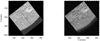 |
Fig. 3. Same as Fig. 2, but for the CLASP-SJ limb pointing. |
| In the text | |
|
Fig. 4. Correlation between He II 30.4 nm and H I 121.6 nm for the November 2, 1998, data set (MXUVI and EIT). The cross on the right indicates the error bars for each data point. The different colored circles on the plot correspond to the intensities of the colored contours in the EIT image (Fig. 1). The dark squares are the Vernazza & Reeves (1978) data from Skylab, shown with their error bars. The solid line fits the MXUVI and EIT data. The dashed line corresponds to the fit from Auchère (2005). |
| In the text | |
|
Fig. 5. Correlation between He II 30.4 nm and H I 121.6 nm for the September 3, 2015, data set (CLASP-SJ and AIA). The plot in the left panel corresponds to the 1.03 arcsec pixel−1 CLASP-SJ resolution, whereas the plot in the right panel has the 10 arcsec pixel−1 MXUVI resolution. The cross on the right of each plot indicates the error bars for each data point. The solid lines correspond to the fit shown in Fig. 4. The dot-dashed lines correspond to the fit of the CLASP (at MXUVI resolution) and AIA data. The dashed lines show the fit for both the MXUVI-EIT and CLASP-AIA data. The colored contours outline the intensity distributions for the different solar regions from Fig. 4. |
| In the text | |
|
Fig. 6. Observations from SUMER at the H I Lyman-β line on April 8, 1996, at 06:09:27 UT (left) and EIT at the He II 30.4 nm line on April 8, 1996, at 06:21:51 UT, corresponding to the SUMER field of view (middle) and the full-disk observation (right). The white square on the full-disk EIT image shows the position of the SUMER field of view. |
| In the text | |
|
Fig. 7. Correlation between He II 30.4 nm from EIT and H I 102.5 nm from SUMER. The cross at the bottom right indicates the error bars for each data point. The solid line is an estimation of the correlation with a linear fit. |
| In the text | |
|
Fig. 8. Distribution of the H I Ly-α/Ly-β intensity ratio from the MXUVI image and the EIT image converted to Ly-β using Eq. (2). The dots and colored circles represent the measurements, which were performed at a period of minimum activity. The colored circles correspond to the different solar regions defined in Fig. 4. In order to maintain SI units, Ly-α intensities are expressed in mW m−2 sr−1, providing numerical values equivalent to the centimeter-gram-second units of erg s−1 cm−2 sr−1 used by Lemaire et al. (2012). The three-dotted-dashed line represents the H I Ly-α/Ly-β intensity ratio deduced from Eqs. (1) and (2). The stars with error bars give an estimate of the accuracy of the ratio. The three other lines are the fits from Fig. 2 of Lemaire et al. (2012). The solid and dashed lines correspond to two quiet-Sun observations, whereas the dotted-dashed line corresponds to a coronal hole. The squares with error bars on these lines give an estimation of the error for different ratio values on the three fits. The large black circles correspond to the ratio deduced from Patsourakos et al. (1998). |
| In the text | |
Current usage metrics show cumulative count of Article Views (full-text article views including HTML views, PDF and ePub downloads, according to the available data) and Abstracts Views on Vision4Press platform.
Data correspond to usage on the plateform after 2015. The current usage metrics is available 48-96 hours after online publication and is updated daily on week days.
Initial download of the metrics may take a while.