| Issue |
A&A
Volume 657, January 2022
|
|
|---|---|---|
| Article Number | A125 | |
| Number of page(s) | 14 | |
| Section | Stellar atmospheres | |
| DOI | https://doi.org/10.1051/0004-6361/202141733 | |
| Published online | 21 January 2022 | |
The CARMENES search for exoplanets around M dwarfs
Diagnostic capabilities of strong K I lines for photosphere and chromosphere★
1
Hamburger Sternwarte, Universität Hamburg,
Gojenbergsweg 112,
21029
Hamburg,
Germany
e-mail: This email address is being protected from spambots. You need JavaScript enabled to view it.
2
Thüringer Landessternwarte Tautenburg,
Sternwarte 5,
07778
Tautenburg,
Germany
3
Institut für Astrophysik,
Friedrich-Hund-Platz 1,
37077
Göttingen,
Germany
4
Centro de Astrobiología (CSIC-INTA), ESAC, Camino Bajo del Castillo s/n,
28692
Villanueva de la Cañada,
Madrid,
Spain
5
Instituto de Astrofísica de Andalucía (CSIC), Glorieta de la Astronomía s/n,
18008
Granada,
Spain
6
Max-Planck-Institut für Sonnensystemforschung,
Justus-von-Liebig-Weg 3,
37077
Göttingen,
Gemany
7
Facultad de Ciencias Físicas, Departamento de Física de la Tierra y Astrofísica; IPARCOS-UCM (Instituto de Física de Partículas y del Cosmos de la UCM), Universidad Complutense de Madrid,
28040
Madrid,
Spain
8
Institut de Ciències de l’Espai (CSIC), Campus UAB, c/ de Can Magrans s/n,
08193
Bellaterra,
Barcelona,
Spain
9
Institut d’Estudis Espacials de Catalunya,
08034
Barcelona,
Spain
10
Landessternwarte, Zentrum für Astronomie der Universität Heidelberg,
Königstuhl 12,
69117
Heidelberg,
Germany
11
Centro Astronómico Hispano-Alemán, Observatorio Astronómico de Calar Alto, Sierra de los Filabres,
04550
Gérgal,
Almería,
Spain
12
Max-Planck-Institut für Astronomie,
Königstuhl 17,
69117
Heidelberg,
Germany
13
Instituto de Astrofísica de Canarias, c/ Vía Láctea s/n,
38205
La Laguna,
Tenerife,
Spain
14
Departamento de Astrofísica, Universidad de La Laguna,
38206
Tenerife,
Spain
15
Centro de Astrobiología (CSIC-INTA), Carretera de Ajalvir,
km 4. 28850 Torrejǿn de Ardoz,
Madrid,
Spain
Received:
7
July
2021
Accepted:
11
October
2021
Abstract
There are several strong K I lines found in the spectra of M dwarfs, among them the doublet near 7700 Å and another doublet near 12 500 Å. We study these optical and near-infrared doublets in a sample of 324 M dwarfs, observed with CARMENES, the high-resolution optical and near-infrared spectrograph at Calar Alto, and investigate how well the lines can be used as photospheric and chromospheric diagnostics. Both doublets have a dominant photospheric component in inactive stars and can be used as tracers of effective temperature and gravity. For variability studies using the optical doublet, we concentrate on the red line component because this is less prone to artefacts from telluric correction in individual spectra. The optical doublet lines are sensitive to activity, especially for M dwarfs later than M5.0 V where the lines develop an emission core. For earlier type M dwarfs, the red component of the optical doublet lines is also correlated with Hα activity. We usually find positive correlation for stars with Hα in emission, while early-type M stars with Hα in absorption show anti-correlation. During flares, the optical doublet lines can exhibit strong fill-in or emission cores for our latest spectral types. On the other hand, the near-infrared doublet lines very rarely show correlation or anti-correlation to Hα and do not change line shape significantly even during the strongest observed flares. Nevertheless, the near-infrared doublet lines show notable resolved Zeeman splitting for about 20 active stars which allows to estimate the magnetic fields B.
Key words: stars: activity / stars: late-type / stars: chromospheres
Full Table 2 is only available at the CDS via anonymous ftp to cdsarc.u-strasbg.fr (130.79.128.5) or via http://cdsarc.u-strasbg.fr/viz-bin/cat/J/A+A/657/A125
© ESO 2022
1 Introduction
The spectra of M dwarfs display several strong K I lines. There is a neutral potassium doublet at 7667.009 Å and 7701.084 Å (vacuum wavelengths), which are denoted as the K I VIS lines here. Moreover, in addition to several weaker K I lines, five strong lines are found at significantly redder wavelengths: the near-infrared (NIR) doublet K I IR lines at 12 435.676 Å and 12 525.591 Å and the K I doublet at 11 693.419 Å and 11 776.060 Å near a companion line at 11 772.859 Å. These potassium lines are known to trace chromospheric activity, but also to be sensitive to photospheric parameters. Furthermore, they are used as diagnostic lines in studies of exoplanet atmospheres (e.g. Burrows & Volobuyev 2003; Sedaghati et al. 2016; Alexoudi et al. 2018; Oshagh et al. 2020).
Chromospheric activity for M dwarfs is most often traced by the Hα line (Gizis et al. 2000; Jeffers et al. 2018), which is easily accessible for these stars. With the advent of spectrographs also covering the NIR, interest arose in new activity-tracing lines in this wavelength range. While the chromospheric He I line at 10 830 Å has been studied thoroughly (Zirin 1982; Sanz-Forcada & Dupree 2008; Andretta et al. 2017; Fuhrmeister et al. 2019), other lines have received less attention. For example, Schmidt et al. (2012) observed emission during large flares in the Paschen lines Paβ, Paγ, and the He I line at 10 830 Å, but Robertson et al. (2016) could not find a correlation of the Paδ line with Hα for time-series observations of the M5.5 V star Proxima Centauri in quiescence. Nevertheless, these authors observed a strong correlation of a combined K I VIS line index with Hα with a Spearman’s rank correlation coefficient of 0.83 and p < 10−45. On the other hand, Kafka & Honeycutt (2006) found an anti-correlation of the absorption strength of the redder optical K I line with Hα comparing stars in the Praesepe open cluster. These latter authors also found the anti-correlation to be more pronounced for the group of early-type M dwarfs rather than for late-type M dwarfs.
The K I VIS lines have additionally been used as exoplanet atmosphere diagnostic (e.g. Sing et al. 2011; Pont et al. 2013; Sedaghati et al. 2016; Alexoudi et al. 2018). On the other hand, K I detection has been highly debated for some planets. For example, a Hubble/STIS detection of potassium in the atmosphere of WASP-31b could not be validated by ground based data (Sing et al. 2015; Gibson et al. 2017; McGruder et al. 2020). Oshagh et al. (2020) caution that even broad band features with a possible origin in atmospheres of exoplanets can actually be caused by stellar activity. Therefore, a good understanding of the activity signatures expected in the K I VIS lines is desirable, but this has never been investigated in detail because of the strong telluric contamination of this region by O2 lines. In a chromospheric activity study of M dwarfs, Schöfer et al. (2019), for example, exclude the K I VIS lines from their analysis of chromospheric tracer lines, which used spectra taken with the CARMENES spectrograph. Precise telluric correction for CARMENES spectra has meanwhile become available (Nagel et al. 2019), and we intend to study not only the K I VIS lines but also the K I IR lines.
Besides use as chromospheric activity tracers, the potassium lines have a large diagnostic potential for photospheric parameters of M stars. The photospheric component of the K I lines is known to undergo strong changes from M to L spectral types, which was described by Kirkpatrick et al. (1999) and Kirkpatrick et al. (1991) for the K I lines doublet at 7700 Å. The general behaviour of these lines was also studied theoretically by Pavlenko et al. (2000) for L dwarfs. The general behaviour of the K I lines in the optical and the near-infrared are the same. For example, a combination of both lines of the K I doublet at 12 435 Å and 12 525 Å was studied by Gorlova et al. (2003). Later, McLean et al. (2007) studied all strong K I lines in the J-band: The two K I IR lines at 11 693 Å and 11 776 Å have approximately the same strength, while the line at 11 772 Å is weaker. For the K I IR doublet at 12 435 Å and 12 525 Å, the redder line is always deeper (McLean et al. 2007). Generally, the K I lines in the optical as well as in the IR broaden to later spectral types. While the lines display nearly no wings in M2.0 dwarfs, wings develop through the M spectral sequence and L dwarfs have extended wings. McLean et al. (2007) found that the line depth and pseudo equivalent width (pEW) also grow along the M type sequence and peak at around mid-L. In contrast, the half width grows until mid-T dwarfs which marked the end of the spectral sequence observed by McLean et al. (2007). The growth of the line width for stars later than M7.0 V can be explained as follows: with decreasing temperatures, the lines should weaken because the transition levels become less populated. However, as dust grains settle more and more below the photosphere, with decreasing temperature the transparency improves. Hence, line formation is observed at much greater depths and pressures (Saumon et al. 2003). With increasing pressure the lines develop broad wings caused by collisional broadening, primarily with H2 molecules (e.g. Burrows & Volobuyev 2003).
Here we study the strong potassium lines K I VIS and K I IR along the M dwarf sequence and their diagnostic potential regarding photosphere and magnetic chromospheric activity. First, we deal with the photospheric parts of the lines and their use as possible stellar parameter indicators. Second, we inspect how activity manifests itself in these lines and if they are sensitive to Zeeman broadening.
Due to the fact that, in M dwarfs, Zeeman splitting often only leads to additional line broadening, radiative transfer models are needed to model the spectra correctly. Nonetheless, magnetic fields have been measured in M stars. For example, Johns-Krull & Valenti (1996) measured the σ components of Zeeman splitting in the wings of a Fe I line at 8468.40 Å in several M dwarfs and was able to detect strong magnetic fields of 3.8 and 2.6 kG in EV Lac and Gliese 729, respectively, with filling factors f of 50 %. Reiners & Basri (2006) used the FeH lines at about 1 μm to classify the magnetic field for 20 M2–M9 dwarfs as weak, intermediate, or strong. For instance, they report Bf > 3.9 kG for YZ CMi, Bf = 2.9 kG for AD Leo, and Bf = 2.3 kG for vB 8. Bf here is the product of the magnetic field B and the filling factor f. Shulyak et al. (2019) made use of a direct magnetic spectrum synthesis to improve this kind of measurement and derived magnetic fields in a sample of 29 M dwarfs using CARMENES spectra.
The paper is structured as follows: in Sect. 2, we present the data, their reduction, and the method for the pseudo-equivalent width measurement. In Sect. 3, we deal first with the usability of the blue optical line in Sect. 3.1, then with the usage of the potassium lines for determination of photospheric parameters in Sect. 3.2, followed by the diagnostic capabilities for stellar activity in Sect. 3.3. There we concentrate on the activity characterisation by correlation with Hα in Sect. 3.3.1, the behaviour during strong flares in Sect. 3.3.2, and the detection of resolved Zeeman splitting in some stars in Sect. 3.3.3. We present concluding remarks in Sect. 4.
2 Observations and measurement method
2.1 Available data and their reduction
All spectra used for the present analysis were taken with the CARMENES spectrograph installed at the 3.5 m Calar Alto telescope (Quirrenbach et al. 2016). CARMENES is a spectrograph covering the wavelength range from 5200 to 9600 Å in the visual channel (VIS) and from 9600 to 17 100 Å in the NIR channel. The instrument provides a spectral resolution of ~94 600 in VIS and ~80 400 in NIR. The CARMENES consortium devoted 750 nights to conducting a survey of ~350 M dwarfs to find low-mass exoplanets (Alonso-Floriano et al. 2015; Reiners et al. 2018). As the cadence of the spectra is optimised for the planet search, usually no continuous time-series are obtained.
In our analysis, we consider a sample of 324 M dwarfs, excluding known close binaries (Baroch et al. 2018; Schweitzer et al. 2019), resulting in a study of about 15 000 spectra taken before July 2020. The stellar spectra were reduced using the CARMENES reduction pipeline (Zechmeister et al. 2014; Caballero et al. 2016). Subsequently, we corrected them for barycentric and radial velocity motions. We carried out a correction for telluric absorption lines (Nagel et al. 2019) using the molecfit package1, but did not correct for airglow emission lines.
Parameters of the pEW calculation.
2.2 Measurement of equivalent width
We measured the pEW of the blue K I VIS line at 7667.009 Å (hereafter K I VISblue) and of the red K I VIS line at 7701.084 Å (hereafter K I VISred), the blue K I IR doublet line at 12435.676 Å (hereafter K I IRblue) and the red K I IR line at 12525.567 Å (hereafter K I IRred), and the Hα line for comparison purposes. The integration ranges and the reference bands for these lines are given in Table 1. The pEW iscalculated using
 (1)
(1)
where Fcore is the flux density in the line band, F0 is the mean flux density in the two reference intervals (representing the pseudo continuum), and λ denotes wavelength. The Hα line allows us to discriminate between active and inactive stars: we define Hα in absorption by pEW(Hα) > − 0.6Å Fuhrmeister et al. (2019) and call these inactive.
We exclude three strong K I lines in the NIR at 11 693.419 Å, 11 772.859 Å, and 11 776.060 Å from our analysis because they are contaminated by OH airglow lines at 11 696.44 Å and 11 771.00 Å (Oliva et al. 2015), which are not corrected by the method of Nagel et al. (2019). Another K I IR line at 11 693.419 Å is heavily blended with an Fe I line at 11 693.176 Å, which can be nearly as strong as the K I line. Finally, the two lines at 11 772.859 Å and 11 776.060 Å are increasingly blended with each other toward the mid- and late M dwarf regime.
To avoid the region heavily contaminated by telluric features bluewards of the K I VISblue line, we choose the same reference region for both doublet lines with one reference region between the two lines and one redwards of the K I VISred line. As photospheric K I lines develop broad wings, we caution that, for stars later than M4.5 V, the reference bands are situated in the far wings of the lines for K I VIS. We used narrow wavelength ranges to compute the pEW only for the line centre, which is most sensitive to activity-related ‘fill-in’ or emission in the line core. The difference between fill-in and emission cores can be best seen in Figs. 5 (bottom panel) and 7 (left panels). Therefore, our integration band is optimised for detecting chromospheric variability, which would be diluted in a setup with broader integration bands optimised for stellar parameter determination. Also, for fast rotators with v sin i > 15 km s−1, all pEWs are underestimated compared to pEWs for the whole line; see Sect. 3.2. We also caution that our pEW is dependent on the resolution of the spectra. In particular, lower resolution is expected to carry photospheric signal into the integration band while narrow chromospheric emission would be blurred out of it. The reverse occurs at higher resolution until the instrumental resolution surpasses the width of the natural spectral features and higher resolution ceases to noticeably affect the spectrum. Because the reference bands are broad, resolution effects are much weaker there. While the details depend on the exact spectral shape, we expect negligible changes in the pEWs as long as the central integration band covers a minimum of three resolution elements. This translates into a minimum resolution of 50 000 for the K I VIS lines and 77 000 for the K I IR lines required to reproduce the pEWs with our setup. Yet, lower spectral resolution and potentially wider bands may of course still yield comparable if not identical results.
Thus, time-series of pEW measurements were obtained for each star. From these pEW time-series, we calculated the median pEW and the median average deviation about the median (MAD), which is a robust estimator of the scatter (Hampel 1974; Rousseeuw & Croux 1993; Czesla et al. 2018). The uncertainty of individual pEW measurements strongly depends on the S/N of the spectra, which may be an issue for Hα and the K I VIS lines. Typically, the S/N is better for bright, early M dwarfs than for fainter mid-type M dwarfs because the maximum exposure time in the survey was 1800 s. We did not compute pEWs when the S/N in the pseudo-continuum was lower than 10, and therefore pEW measurements of the Hα line are missing for some of the latest M dwarfs.
2.3 Stellar parameters
In the following, we compare our measured pEWs to effective temperatures, Teff, surface gravity, log g, and metallicity [Fe/H]. As stellar parameters already exist for all our sample stars, we refrained from computing these by ourselves and instead used the ones reported by Schweitzer et al. (2019), who employed the method of Passegger et al. (2018). These two studies used PHOENIX photospheric models published by Husser et al. (2013) to derive the stellar parameters based on fits to CARMENES spectra. We show two of their best-fit PHOENIX models in Fig. 1, which demonstrates the good fit of the models in the wings. The line core, however, can be influenced by chromospheric activity, which is not taken into account in the (purely photospheric) spectral models.
3 Results
3.1 Usability of the K I VISblue line
For the K I VIS doublet, the blue line is much more prone to telluric line contamination than the red line, which provides an opportunity to test the telluric correction. To that end, we compare relative variability observed in the line cores as measured by the variation in pEW(K I VISblue) and pEW(K I VISred). In particular, we investigate the respective MADs, which we show as a function of MAD(Hα) in Fig. 2. The MAD of pEW(K I VISblue) is typically higher than that for the red line. Such high variations in any of the K I VIS lines are not expected, particularly for the inactive stars with little variation in Hα.
Several factors can contribute to the total scatter observed in the lines. First, we consider statistical noise with variance,  , where x denotes either r or b to identify the red and blue K I lines. This term represents measurement noise and instrumental effects. Second, activity contributes to the scatter of pEW measurements, which we name
  . Third, inaccuracies in the telluric correction can add to the observed scatter, which we summarise in the term
  . Assuming that these terms are independent and approximately Gaussian, their variances can be added together, so that we obtain
 (2)
(2)
The statistical variances are equal for both lines as can be seen from the very similar statistical errors for the flux density in both lines. Similarly, the emission oscillator strengths or, equivalently, Einstein coefficients for spontaneous emission are almost identical. As the lines both form in the same chromospheric regions, this implies that activity-induced emission for both lines is also very similar, and so the activity-related variances can also be assumed to be equal. Given that the red line suffers from marginal telluric contamination, we assume  and it follows that the observed excess scatter in pEW(K I VISblue) is attributable to the telluric variance term,
  . This is consistent with the correlation between pEW(K I VISblue) and pEW(K I VISred) tending to be weak for the time-series of the stars with excess scatter in pEW(K I VISblue). We therefore only use the K I VISred line in our further analysis.
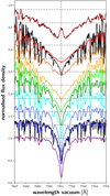 |
Fig. 1 Spectral subtype sequence for the wavelength region around K I VISred. There is an offset added to the normalised spectra for convenience, which is larger for the M7.0 spectrum. For comparison we show PHOENIX models in black for two of the stars; more details are given in the main text. The shown spectra correspond to the following stars from bottom to top (Karmn number and corresponding line colour in parenthesis): M0.0 V: HD 23453 (J03463+262, purple); M1.0 V: GJ 2 (J00051+457, blue); M2.0 V: GJ 47 (J01013+613, dark blue); M3.0 V: G 244-047 (J02015+637, cyan); M4.0 V: LP 768-113 (J01339–176, green); M4.5 V: YZ Cet (J01125–169, lime green); M5.5 V: GJ 1002 (J00067–075, orange); M6.0 V: CN Leo (J10564+070, brown); M7.0 V: Teegarden’s Star (J02530+168, red); M8.0 V: vB 10 (J19169+051S, dark red). |
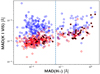 |
Fig. 2 MAD(K I VISred) (red open circles) and MAD(K I VISblue) (blue open circles) as a function of MAD(Hα). Black symbols denote the dwarfs with a correlation between pEW(K I VISred) and pEW(Hα) as defined in Sect. 3.3.1. The dashed vertical line marks the gap between weakly and strongly variable stars, which corresponds roughly to inactive and active stars. |
3.2 Line profile development with spectral type and gravity
As predicted by synthetic spectra, we observe a strong dependence of pEW(K I VIS) and pEW(K I IR) on Teff. In Fig. 1, we show a spectral sequence of line profiles of the K I VISred line, which shows the development of broad wings towards later spectral types. Moreover, excess emission may be distinguished in the lines cores in subtypes of M5.5 V stars and later, which is discussed in more detail in Sect. 3.3.2. The K I IR lines also broaden toward later spectral types, but no systematic appearance of emission cores for the latest spectral types is observed. However, some stars show line shapes reminiscent of chromospheric emission cores, which is discussed in more detail in Sect. 3.3.3.
In Fig. 3, we show a comparison between pEW(K I VIS) and Teff (as determined by Schweitzer et al. 2019). A close linear relation is apparent for all but the earliest M dwarfs with Teff ≥ 3600 K. For comparison we also show pEW(K I VISred) calculated from PHOENIX spectra from the library by Husser et al. (2013). The deviation between the PHOENIX spectra and observationsin the line core may be attributed to two factors: First, the photospheric models are calculated using local thermal equilibrium (LTE), which may lead to small deviations in the core compared to non-LTE models. This may apply for the smaller deviation in the K I IR lines. Second, the models do not include any activity. As the K I IR lines react less to activity as detailed in Sect. 3.3.1, activity may account for the larger systematic deviation between PHOENIX and observed spectra in the K I VISred line. As there seems to be a shift of about 200 K between models and observations, this may indicate that the K I VISred line has a chromospheric contribution even for inactive stars and is formed in the lower chromosphere.
Observed outliers are due to several factors: (i) fast rotation. We mark stars with v sin i > 15 km s−1. Fast rotation flattens the line profiles and causes the lower pEW measurements as we focus only on the line centre. Many of these objects are also young (age below 100 Ma), and therefore subject to low gravity, which may also decrease their pEW. (ii) Chromospheric activity. We also mark stars of type M5.0 V and later with a measured v sin i of 2 km s−1 or more. While chromospheric emission cores are noted only at M5.5 V and later, some chromospheric contribution sets in at M5.0 V already. (iii) Miscorrections of telluric lines or spectral misalignment. This explains in particular all non-marked outliers with pEW(K I VIS) values lower than 0.3 Å. Therefore, we exclude pEW(K I VIS) below this threshold from the following considerations; also we exclude all outliers caused by fast rotation or chromospheric activity. In this case, the relation between Teff and pEW(K I VIS) for the 194 stars fulfilling also 3000 K < Teff < 3600 K leads to a Pearson’s correlation coefficient of −0.91, formally corresponding to a p-value of 10−78. The relation can be described by a linear regression of the form
 (3)
(3)
leading to a standard deviation of Teff,K i VIS red − TSchw19 of 55 K.
A similar trend is observed for the pEW(K I IRred), but again for Teff > 3600 K a reversal in pEW(K I IRred) is observed as shown in Fig. 3. Applying again a linear regression leads to the relation
 (4)
(4)
which yields a standard deviation of 64 K for Teff,K i IR red − TSchw19. The value of Pearson’s correlation coefficient is −0.88 with a p-value of 10−66.
If the effective temperature, Teff, is replaced by log g as the dependent variable, a similar relation is found for the slowly rotating main sequence dwarfs. For stars with 3600 K > Teff > 3000 K this can be seen in Fig. 4 with a reversal for stars with higher temperatures. This similarity in the behaviour is expected, because the effective temperature and surface gravity are not independent variables for main sequence stars as detailed for example in Schweitzer et al. (2019).
The value of the Pearson’s correlation coefficient between pEW(K I VISred) and log g is 0.95 with a p-value of 10−102. The best-fit relation is given by
 (5)
(5)
with std(loggK I VIS red- loggSchw19) = 0.06 dex. For pEW(K I IR), a somewhat less pronounced correlation is found with Pearson’s correlation coefficient yielding 0.81 and a p-value of 10−46. The best-fit relation reads
 (6)
(6)
and std(log gK I IR red- log gSchw19) = 0.09 dex.
Finally, we compared pEW(K I VIS) and pEW(K I IR) to the metallicity [Fe/H] also determined by Schweitzer et al. (2019), but could not identify any relation similar to the ones presented above. We show our comparison in Fig. A.1. The Pearson’s correlation coefficient between [Fe/H] and pEW(K I VIS) is –0.06 with a p-value of 0.40, and for pEW(K I IR) it is 0.24 with a p-value of 0.0004. Though the latter p-value formally indicates a correlation, it is much weaker than for Teff or log g. Also computing a linear regression as above leads to a standard error of 0.17 dex in the thus-determined [Fe/H]. As the [Fe/H] values in our sample (again not considering the outliers) range only from –0.34 dex to 0.17 dex, we do not consider a formal fit to be useful.
Therefore, in summary, a comparison with the results by Schweitzer et al. (2019) demonstrates that for effective temperatures in the range 3000 < Teff < 3600 K, the K I VIS and K I IR lines alone allow a good estimate of temperature and log g, while an estimation of the metallicity is not possible with the data.
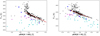 |
Fig. 3 Effective temperature Teff as a functionof pEW(K I VISred) (left) and pEW(K I IRred) (right). Stars marked in magenta are fast rotators with vsini >15 km s−1. Stars marked in cyan have spectral type M5.0 V or later and have measurable v sin i > 2 km s−1. Blue circles mark the pEW as calculated from PHOENIX spectra taken from Husser et al. (2013). |
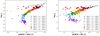 |
Fig. 4 log g as a functionof pEW(K I VISred) (left) and pEW(K I IRred) (right), respectively, and effective temperature colour coded for both cases. |
3.3 K I VIS and K I IR lines as activity tracers
The values of pEW(K I VIS) cannot be used as a direct activity indicator because they strongly depend on spectral type and are dominated by photospheric contributions. This combination prevents comparison between stars of different spectral type and also makes subtraction of a quiescent template challenging. As an illustration, we show the dependence of pEW(K I VIS) on pEW(Hα) for each spectral type in Fig. B.1.
As shown in Fig. 2 and discussed further in Sect. 3.3.1, the values of MAD(pEW(K I VISred)) are correlated with MAD(pEW(Hα)). In particular, we find a value of 0.6 for the Pearson’s correlation coefficient and a p-value of 10−31, suggesting a chromospheric origin of the variations. We do not consider pEW(K I VISblue) because of the remaining telluric contamination for many stars. Moreover, when considering MAD(pEW(K I IR)), we do not find a correlation to MAD(pEW(Hα)), showing the relative insensitiveness of the K I IR lines to stellar activity. We show our findings for MAD(pEW(K I IR)) in Fig. B.2.
3.3.1 Correlation with the Hα line
Making use of our time-series measurements, we search for possible (anti-)correlation of pEW(K I VISred) and pEW(K I IR) with pEW(Hα) in individual stars. The relevant measurements are listed in Table 2 with the full table available at CDS. In particular, the table gives a common name and also the CARMENES identification, Karmn, of each star and the value of the Pearson’s correlation coefficient between pEW(K I VIS) and pEW(Hα) along with the corresponding p-value. Moreover, Table 2 lists the median(pEW) and the MAD for Hα, the red and blue K I VIS lines, and the red and blue K I IR lines.
A pertinent example of correlation between the K I VISred and Hα line indices is observed in the M6.5 V star DX Cnc (Karmn: J08298+267), shown in Fig. 5. As may be expected, this late-type M star displays Hα emission along with an emission core in the K I VISred lines. Additionally, there is variation in K I VIS (Fig. 5). While the values of pEW(K I VISred) correlate very well with pEW(Hα), the correlation between pEW(K I VISblue) and this latter is weaker. The values of the Pearson’s correlation coefficient are 0.97 and 0.57 with p-values of 10−13 and 0.004, respectively. In contrast, neither the red nor blue component of the K I IR lines shows a significant correlation with Hα, yielding P-values larger than 0.4. We show the time-series, the correlation plot, and the spectra of the K I IR lines for DX Cnc in Fig. B.3.
To study correlations in the whole sample, we first screen the time-series based on the correlation coefficient between pEW(K I VISred) and pEW(Hα). In particular, we consider index time-series with a Pearson’s correlation coefficient of |r| > 0.4 and p < 0.005 to be good candidates for correlated evolution. A total of 59 stars match this criterion.
In a next step, we review the time-series matching the criterion by eye. This visual inspection revealed that out of the 59 candidates, 7 can be attributed to outliers in the time-series. The MADs for the 52 stars with visually confirmed correlation are plotted in Fig. 2.
For the K I IR lines, we find only five stars where both lines correlate with pEW(Hα). Again, visual inspection shows that one is attributable to outliers in its time-series. One of the four remaining stars (AD Leo) shows positive correlation and three stars (Ross 1020, GJ 1254, and Ross 271) show negative correlation. All four stars show the same behaviour in the K I VISred line. Overall, we find about ten times fewer examples of correlation or anticorrelation for the K I IR lines compared to the K I VISred line, indicating their relative insensitivity to chromospheric activity.
For both, the K I VIS and K I IR lines, examples of positive correlation and anti-correlation are found. For the K I VISred and the K I IR lines, we find that anti-correlation is typical for weakly variable stars, defined here as those with MAD(Hα) < 0.07 Å. This corresponds to the apparent gap in Fig. 2, which also roughly separates active stars with Hα in emission from stars with Hα in absorption. For stars with Hα in emission we find only positive correlation, while for stars with median(pEW(Hα)) > –0.6 Å we find three stars (Teegarden’s star, GJ 1093, and Ross 619) that nevertheless exhibit a positive correlation. This may be related to the late spectral type of these stars (M4.5–7.0 V), because all correlating stars with these spectral types show a positive correlation.
The observed behaviour agrees well with the results of Kafka & Honeycutt (2006) and Robertson et al. (2016), who found that early-type inactive M stars show an anti-correlation between pEW(K I VIS) and pEW(Hα), while activelate-type M dwarfs show a positive correlation. For the latter stars, Hα is normally in emission and higher activity corresponds to fill-in or more emission in the emission cores of the K I VIS lines. For the early-type inactive stars, Hα is normally in absorption and a fill-in is apparently accompanied by deepening of the K I VIS lines.
The least active among the active stars do not show a correlation between these two lines, which we attribute to a lower sensitivity of the K I VIS lines to changes in activity compared to Hα. Therefore, we computed a linear regression to determine the slope between pEW(K I VIS) and pEW(Hα). While for the early-type stars, we find slopes of between −0.01 and −0.10, the majority of the later type stars have slopes of between 0.003 and 0.01 with seven stars showing significantly higher slopes of between 0.01 and 0.02. While the fits of the slopes appear statistically meaningful, the cause for the steeper slopes remains elusive. For the four stars showing a correlation between pEW(K I IR) and pEW(Hα), we find comparable slopes between these lines.
The relation between the slope (of the linear regression between pEW(Hα) and pEW(K I VISred)) and Teff can be seen in Fig. 6, where the transition from negative to positive slope takes place at Teff~ 3400 K corresponding to spectral types of M3.0 V–M4.0 V. This transition from negative to positive slope may be explained by the different origin of the Hα and the K I VIS lines. While Hα originates in plages in the upper chromosphere or even the lower transition region, the K I VIS cores should originate in the lower chromosphere, as was found for the Na I D lines by Andretta et al. (1997). If the K I VIS core originates as an absorption line in spots, and higher activity levels lead to an increase in the area of spots, this would lead to a deepening line. In contrast, higher activity levels lead to more Hα emission in the upper chromosphere causing a fill-in of an Hα absorption line and therefore explaining the anti-correlation with the K I VIS line. For the late-type stars, Hα becomes an emission line, which is collisionally controlled. The same should be true for the K I VIS line, because for the late stars, which exhibit K I VIS in emission, the densities in the lower chromosphere should be quite high. As the photospheric background is also low, this emission shows up as emission cores correlated with Hα emission.
The right panel of Fig. 6 also shows that the slope of the linear regression depends on the variability of the star as measured by MAD(Hα). For anti-correlation, the slope is flattening for higher variability, while for correlation the slope is much less dependent on the MAD(Hα) and seems to be saturating at around 0.02.
The above findings indicate that K I VIS lines, and in particular the K I IR lines, are less sensitive to activity than Hα. Surprisingly, the later-type, more variable stars with Hα in emission show an even lower sensitivity of K I VIS compared to Hα than stars with Hα in absorption. This may be caused by a higher sensitivity of Hα emission lines to changes in the chromosphere compared to Hα absorption lines.
For the 16 stars of spectral type M6.0 V and later, our sample unfortunately only comprises three stars with sufficient S/N in Hα in the individual spectra to compute pEW(Hα). Therefore, we cannot compute the correlation between pEW(Hα) and pEW(K I VISred) for most of these stars. As they all show emission cores in the K I VISred lines, we nevertheless assume that for all of these stars a positive correlation exists. If this is true, the favourable redder location of the K I VIS lines can make the pEW(K I VIS) a valuable substitute for pEW(Hα).
Also, we caution that we do not identify all stars with a correlation between pEW(Hα) and pEW(K I VISred), because some stars fail our correlation criterion because of outliers in their time-series. These outliers may even be caused by flaring activity, where the K I VISred line may exhibit a different reaction to the flare than Hα, therefore diluting the correlation. An example is the M5.5 V star GJ 1002, where two flares weaken the correlation seen in the K I VISred line. Another reason for not finding existing correlations in the inactive stars may also be the constant activity level of these stars during observations, when even the Hα line shows no variation. This latter case applies to many of our sample stars. In particular, we deem all stars with MAD(pEW(Hα)) < 0.01 Å to be too constant to find a correlation. For the two stars in this regime, where we nevertheless find an anti-correlation, the slope is extraordinarily low and they both have more than 80 observed spectra. There are 67 (20%) stars in this low-variation regime.
Measured median pEWs, MADs, and correlation coefficients of the considered line.
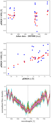 |
Fig. 5 DX Cnc time-series (top) and correlation plot (middle) for K I VISred (red circles) and K I VISblue (blue circles), and all spectra around the central wavelength of the K I VISred line, marked with a dashed line (bottom). |
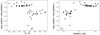 |
Fig. 6 Slope of the linear regression of pEW(Hα) and pEW(K I VISred) as function of effective temperature (left) and of MAD(Hα) (right). |
3.3.2 Variability during flares
Due to the observing scheme of CARMENES, which is optimized for planet detection, consecutive spectra exist so rarely, that the snapshot character of most of the spectra prevents us from identifying the characteristic exponential decay seen in flare light curves. Thismakes flare detection rather challenging. Nevertheless, large flares can be detected as ‘outliers’ in Hα or by asymmetries in the line shape as demonstrated for example by Fuhrmeister et al. (2018, 2020). During these flares, the K I VIS lines shows fill-in. Only for the M5.0 V star 1RXS J114728.8+664405 (Karmn: J11474+667) is a clear emission core identified. For the most part, it is the slightly cooler stars with spectral type M5.5 V that start to develop emission cores in the K I VIS lines also in quiescence. As shown in Fuhrmeister et al. (2008) using VLT/UVESobservations, CN Leo also exhibits an emission core in the K I VIS lines during a mega flare, but not during quiescence also covered by these data. In our CARMENES observations, CN Leo shows an emission core in the average spectrum, but not in every individual spectrum, which indicates that the K I VIS emission is variable.
We show two instructive examples of flare spectra in Fig. 7. In the bottom panel, we display some of our spectra of EV Lac (Karmn: J22468+443), including the spectrum taken at JD 2457633.46711 d, which corresponds to the largest flare of this star in the time-series. The behaviour of other chromospheric indicator lines during this flare has been described in Fuhrmeister et al. (2018, 2020), as well as the appearance of large red asymmetries in Hα and other lines. Here, the K IVISred line spectrum also shows this red asymmetry, which is most probably caused by mass motions.
Another example of a strong flare affecting the K I VISred line is shown in the top panel of Fig. 7 for spectra of 1RXS J114728.8+664405. One flare leads to a strong fill-in, while the second flare leads to an emission core. How this different reaction of the line shape is caused remains unknown: Hα exhibits strong red asymmetries for both flares, with the main difference being the amplitude of the Hα line. Comparison spectraof Hα and the He IIR line can be found again in Fuhrmeister et al. (2020) for the flare marked in blue in Fig. 7. The other flare has been observed more recently and is not included in the study by Fuhrmeister et al. (2020).
In contrast to the K I VIS lines, no clear variability is found in the K I IR lines, not even during the largest flares in EV Lac or 1RXS J114728.8+664405 as can be seen for EV Lac in Fig. 7. While the redder of the absorption dips of the line shows some deformation during the flare, the bluer dip does not. Though we cannot rule out some reaction to the flare, we think this is most probably noise, because the line centre does not show any variation.
This non-reaction to flares strongly suggests that the correlation or anti-correlation found between the pEW(K I IR) and pEW(Hα) for the four stars mentioned above is caused by some alternative mechanism to that causing the correlation between pEW(K I VISred) and pEW(Hα). Possible alternative mechanisms are: (i) The K I IR lines may originate not from the chromosphere, but mainly from photospheric spots, whose relative area should also be roughly correlated with Hα activity but would not change during flares. (ii) As the K I IR lines are magnetically sensitive as detailed in the following section, changes in the magnetic field may change the shape of these lines and therefore lead to variations in pEW(K I IR). If pEW(Hα) correlateswell with the magnetic field, a correlation with pEW(K I IR) should also appear.
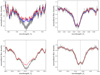 |
Fig. 7 K I VISred (left) and K I IRblue (right) spectra of 1RXS J114728.8+664405 (top) and EV Lac (bottom) during quiescence (grey lines) and flares (red and blue lines). In contrast to the K I VISred line, the K I IRblue line does not appear to react to flares. The double dip structure of the K I IRblue line is explained in Sect. 3.3.3. |
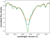 |
Fig. 8 Spectra of the M5.0 V stars G 177-025 (blue), LP 731-076 (orange), and GJ 1028 (green), depicting the different line shapes found (flat bottom, double dip structure, and unperturbed). |
3.3.3 Zeeman effect
For about 20 active stars in our sample, the K I IR lines show a double minimum structure imitating an emission core. While this profile resembles a chromospheric emission line core, we do not observe any flare-induced variability. For example, the large flare on EV Lac (see Sect. 3.3.2) leads to considerable fill-in in the K I VIS lines, as seen in Fig. 7, but does not clearly affect the profiles of the K I IR lines. Also, chromospheric computational models, such as those constructed by Hintz et al. (2019) for M2–3 dwarfs using PHOENIX, do not show any emission cores or noteworthy fill-in for the K I IR line profiles, even for extreme flaring models.
These considerations lead us to the hypothesis that the line profile is caused by magnetic Zeeman splitting. This would also explain thatfor nearly all stars with a double dip structure, the line profile of the K I IR lines is slightly broadened compared to inactive stars of the same spectral type, which show a ‘normal’ single dip line-shape. Also, in comparison to the chromospheric models by Hintz et al. (2019), who treats K I in non-LTE, the observed line profiles are broader than the profiles of the model spectra. Additionally, Shulyak et al. (2019) also used CARMENES spectra to determine magnetic fields in 29 stars using direct magnetic spectrum synthesis. Five of the stars, where we identify the peculiar double dip structure are also part of this study. We find for these five stars that the distance between the two dips grows with measured magnetic field.
Finally, we found the line profile of the K I IR lines to have a ‘flat bottom’ (a trough-like shape) in a number of stars. Examples are the stars LTT 11262, 2M J07000682-1901235, and G 177-025. Typical examples of a flat bottom, a double dip structure, and an unperturbed line can be found in Fig. 8. Measurements by Shulyak et al. (2019) for two stars with a flat bottom line shape show that their magnetic fields are of approximately the same magnitude as the stars with the double dip structure, but the same two stars have larger v sin i values in comparison. Therefore, the flat bottom may indicate unresolved Zeeman splitting, which represents the typical case for M dwarfs, while the double dip structure is due to resolved Zeeman splitting. Resolved Zeeman splitting has been used more frequently to measure field strengths in chemically peculiar early-type stars (e.g. Chojnowski et al. 2019).
In the case of resolved Zeeman splitting, the (half-)width of magnetic line splitting, Δλ, is characterised by the Landé factor, gi. In particular, the magnetic field strength B in kG is related to the split by
 (7)
(7)
where Δλ is the split in wavelength in Å (Reiners 2012). Therefore, NIR lines show greater splitting because of the quadratic dependence on wavelength. To compute the magnetic field B, the Landé factor for the line transition is required, but no experimental Landé factors are known for the K I IR line. Landé factors can be estimated with the formula given by Reiners (2012):
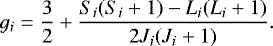 (8)
(8)
Here, S is the spin, L is the orbital angular momentum, and J is the total angular momentum quantum number, and i denotes the level (here upper and lower). Here, the two energy levels of the transition each split into two components because of spin-orbit coupling, i.e. the anomalous Zeeman effect. The Landé factors of the upper and lower energy levels for the K I IRblue line are gup = 2.0 and glow = 0.67, and for the K I IRred line gup= 2.0 and glow = 1.33, respectively.In this case, the Zeeman pattern of the spectral line only consists of components that are shifted with respect to the undisturbed wavelength, but no undisturbed component remains. The resulting pattern for the K I IRblue line is shown in Fig. 9 for different field strengths and a radial field geometry. Because all Zeeman components are shifted, the pattern develops an inversion in the centre at field strengths larger than ~ 1 kG. This inversion is reminiscent of central line emission and is more pronounced in stronger fields.
The K I VIS doublet also shows a similar pattern of Landé factors, which would lead in principle to a double dip structure in these lines as well. However, the shorter wavelength of the K I VIS lines leads to a much narrower Zeeman pattern, which prevents any observations.
The exact evaluation of the magnetic field should be performed using detailed radiative transfer calculations, which is beyond the scope of this paper. We nevertheless attempted some forward modelling of the Zeeman effect using the spectrum synthesis code MAGNESYN (Shulyak et al. 2017), which solves the radiative transfer equations for all four Stokes parameters and a given magnetic configuration. The code is part of the LLMODELS suite described in Shulyak et al. (2004) and was used by Shulyak et al. (2019) to derive magnetic fields for CARMENES spectra.
We show an example of forward modelling for the K I IRblue line in Fig. 10 for the star YZ CMi (Karmn: J07446+035). For this star, the magnetic field was determined by Shulyak et al. (2019) to be < B >= 4.6 ± 0.3 kG with a weakzero-field component. Using a model consistent with the findings by Shulyak et al. (2019) leads to the well-fitting model shown in Fig. 10. The same model leads to no double dip feature in the K I VISred line as expected from our considerations above.
 |
Fig. 9 Stokes I (solid lines) and Stokes V (dashed lines) for the K I IRblue line for different magnetic field strengths computed for a purely radial field. |
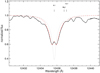 |
Fig. 10 Forward modelling of the Zeeman splitting in the K I IRblue line. Shown is the observed spectrum of YZ CMi in black. The dotted grey line is a radiative transfer model without magnetic field. The red dashed line has been computed with a magnetic field consistent with that found by Shulyak et al. (2019). Atomic lines used in the models are marked at the top. |
4 Conclusions
We present a study of the K I VIS and K I IR doublet lines in a sample of 324 M dwarfs, using a total of more than 15 000 spectra observed within the CARMENES exoplanet survey. Both doublets show prominent photospheric lines across the M dwarf sequence, the profiles of which strongly depend on effective temperature and also on gravity.
We determine pEWs for the line cores of the K I VIS and K I IR lines in band passes optimised for the study of chromospheric activity, which also allow us to deduce relations between pEW, Teff, and log g, for slow rotators with v sin i < 15 km s−1. As the pEWmeasurements for the blue line component of the K I VIS doublet can be affected by telluric correction artefacts, we only consider the K I VISred line for variability studies.
We find that stars later than spectral type M5.0 V exhibit an emission core in the K I VIS lines. Throughout the M dwarf sequence, we find 52 (16%) stars that show a close correlation or anti-correlation between pEW(K I VIS) and pEW(Hα). While stars with stronger variability – which normally also show Hα in emission and are of spectral type later than about M3.0 V – tend to show a positive correlation between pEW(K I VIS) and pEW(Hα), less-variable, inactive early-type stars show an anti-correlation. This is in agreement with the findings of Kafka & Honeycutt (2006), who found an anti-correlation between pEW(K I VIS) and pEW(Hα) for early M dwarfs, and Robertson et al. (2016), who found a correlation for two late-type M dwarfs. For the K I IR lines, we also find four (1%) cases of correlation or anti-correlation with Hα. The potassium lines are significantly less sensitive to chromospheric variability than Hα, and for the more active stars with Hα in emission the difference seems to be even more severe, which we ascribe to an increased sensitivity of the pEW(Hα) to variability for these stars. This low sensitivity of the K I VIS lines to activity-related variability in comparison to Hα – which is particularly pronounced for the K I IR lines – favours their usage in transmission spectroscopy of exoplanetary atmospheres. Also, the magnetic splitting pattern detected for the K I IR lines did not show significant changes in our data, especially not during flares, where changes in the magnetic field due to reconnection may be expected. Whether or not long-term variation of the magnetic field – especially with slow rotation or cycles – leads to changes in the line profiles remains to be investigated, but changes on these timescales should not affect transmission spectroscopy.
During strong flares, the K I VIS lines show a pronounced fill-in or development of an emission core for spectral types around M5.0 V. However, the K I IR line profiles do not show a significant change during these transient events. Nevertheless, the K I IR lines are sensitive to the stellar magnetic field. The line shape often exhibits a double dip structure for active stars, which we attribute to resolved anomalous Zeeman splitting caused by a symmetric split by the π- and σ-components. We therefore find that the K I IR lines are an important new diagnostic of magnetic fields in M dwarf stars.
Acknowledgements
B.F. acknowledges funding by the DFG under Schm 1032/69-1. CARMENES is an instrument for the Centro Astronómico Hispano-Alemán de Calar Alto (CAHA, Almería, Spain). D.S. acknowledges the financial support from the State Agency for Research of the Spanish MCIU through the “Center of Excellence Severo Ochoa” award to the Instituto de Astrofísica de Andalucía (SEV-2017-0709) We acknowledge financial support from the Agencia Estatal de Investigación of the Ministerio de Ciencia, Innovación y Universidades and the ERDF through projects PID2019-109522GB-C5[1:4]/AEI/10.13039/501100011033 PGC2018-098153-B-C33 and the Centre of Excellence “Severo Ochoa” and “María de Maeztu” awards to the Instituto de Astrofísica de Canarias (CEX2019-000920-S), Instituto de Astrofísica de Andalucía (SEV-2017-0709), and Centro de Astrobiología (MDM-2017-0737), and the Generalitat de Catalunya/CERCA programme. CARMENES is funded by the German Max-Planck-Gesellschaft (MPG), the Spanish Consejo Superior de Investigaciones Científicas (CSIC), the European Union through FEDER/ERF FICTS-2011-02 funds, and the members of the CARMENES Consortium (Max-Planck-Institut für Astronomie, Instituto de Astrofísica de Andalucía, Landessternwarte Königstuhl, Institut de Ciències de l’Espai, Institut für Astrophysik Göttingen, Universidad Complutense de Madrid, Thüringer Landessternwarte Tautenburg, Instituto de Astrofísica de Canarias, Hamburger Sternwarte, Centro de Astrobiología and Centro Astronómico Hispano-Alemán), with additional contributions by the Spanish Ministry of Economy, the German Science Foundation through the Major Research Instrumentation Programme and DFG Research Unit FOR2544 “Blue Planets around Red Stars”, the Klaus Tschira Stiftung, the states of Baden-Württemberg and Niedersachsen, and by the Junta de Andalucía.
Appendix A Relation of [Fe/H] to pEW(K I VISred) and pEW(K I IRred)
Figure A.1 shows the distribution of [Fe/H] over pEW(K I VISred) and pEW(kirr), respectively. No relation is found.
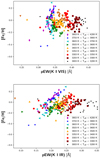 |
Fig. A.1 [Fe/H] as a function of pEW(K I VISred) (top) and pEW(K I IRred) (bottom). |
Appendix B The pEW(K I VISred) and pEW(K I IRred) as activity indicators
We additionally show the dependency of pEW(K I VISred) on pEW(Hα) for all slow rotators with vsini < 15 km s−1 in Fig. B.1. We exclude faster rotators because the flattening of the spectral lines by rotation would lead to a larger effect on the pEW. For the inactive stars with pEW(Hα) > − 0.6Å, the M0.0 V and M1.0 V stars form a cloud-like structure, while later type stars form linear segments. We therefore argue that the dependency for these stars is mainly caused by the temperature dependency and that pEW(K I VISred) is not a good activity tracer for such spectral types, at least not for comparison between stars. The same applies to the K I IRred lines for the inactive stars. Similarly, for the active stars, no clear correlation between pEW(Hα) and pEW(K I VISred) is seen. Indeed the deepest lines with the largest pEW(K I VISred) are measured for the inactive stars of each spectral subtype. While the pEW(K I VISred) for the active stars seem to be approximately constant, for the pEW(K I IRred) a weak correlation is observed with pEW(Hα) indicating some sensitivity to activity.
Moreover, as a comparison to Fig. 2 we show in Fig. B.2 the relation between MAD(K I IR) and MAD(Hα).
For comparison with Fig. 5, we show for the star DX Cnc the time-series for the K I IR lines, their correlation to pEW(Hα), and the spectra of the K I IRblue line in Fig. B.3.
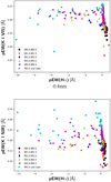 |
Fig. B.1 Dependency of pEW(K I VISred) (top) and pEW(K I IR r) (bottom) on pEW(Hα) for different spectra types for all stars with vsini < 15 km s−1. |
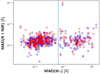 |
Fig. B.2 Same as Fig. 2, but for the K I IRred (red circles) and the K I IRblue (blue circles) line.The two outliers at the top are caused by the same star, which has only four measurements, out of which two happen to be compromised by low S/N, which leads to the large MAD(K I IR) values. |
References
- Alexoudi, X., Mallonn, M., von Essen, C., et al. 2018, A&A, 620, A142 [NASA ADS] [CrossRef] [EDP Sciences] [Google Scholar]
- Alonso-Floriano, F. J., Morales, J. C., Caballero, J. A., et al. 2015, A&A, 577, A128 [NASA ADS] [CrossRef] [EDP Sciences] [Google Scholar]
- Andretta, V., Doyle, J. G., & Byrne, P. B. 1997, A&A, 322, 266 [NASA ADS] [Google Scholar]
- Andretta, V., Giampapa, M. S., Covino, E., Reiners, A., & Beeck, B. 2017, ApJ, 839, 97 [Google Scholar]
- Baroch, D., Morales, J. C., Ribas, I., et al. 2018, A&A, 619, A32 [NASA ADS] [CrossRef] [EDP Sciences] [Google Scholar]
- Burrows, A., & Volobuyev, M. 2003, ApJ, 583, 985 [Google Scholar]
- Caballero, J. A., Guàrdia, J., López del Fresno, M., et al. 2016, in Proc. SPIE, 9910, Observatory Operations: Strategies, Processes, and Systems VI, 99100E [Google Scholar]
- Chojnowski, S. D., Hubrig, S., Hasselquist, S., et al. 2019, ApJ, 873, L5 [NASA ADS] [CrossRef] [Google Scholar]
- Czesla, S., Molle, T., & Schmitt, J. H. M. M. 2018, A&A, 609, A39 [NASA ADS] [CrossRef] [EDP Sciences] [Google Scholar]
- Fuhrmeister, B., Liefke, C., Schmitt, J. H. M. M., & Reiners, A. 2008, A&A, 487, 293 [NASA ADS] [CrossRef] [EDP Sciences] [Google Scholar]
- Fuhrmeister, B., Czesla, S., Schmitt, J. H. M. M., et al. 2018, A&A, 615, A14 [NASA ADS] [CrossRef] [EDP Sciences] [Google Scholar]
- Fuhrmeister, B., Czesla, S., Hildebrandt, L., et al. 2019, A&A, 632, A24 [NASA ADS] [CrossRef] [EDP Sciences] [Google Scholar]
- Fuhrmeister, B., Czesla, S., Hildebrandt, L., et al. 2020, A&A, 640, A52 [NASA ADS] [CrossRef] [EDP Sciences] [Google Scholar]
- Gibson, N. P., Nikolov, N., Sing, D. K., et al. 2017, MNRAS, 467, 4591 [NASA ADS] [CrossRef] [Google Scholar]
- Gizis, J. E., Monet, D. G., Reid, I. N., et al. 2000, AJ, 120, 1085 [Google Scholar]
- Gorlova, N. I., Meyer, M. R., Rieke, G. H., & Liebert, J. 2003, ApJ, 593, 1074 [NASA ADS] [CrossRef] [Google Scholar]
- Hampel, F. R. 1974, J. Am. Stat. Assoc., 69, 383 [Google Scholar]
- Hintz, D., Fuhrmeister, B., Czesla, S., et al. 2019, A&A, 623, A136 [NASA ADS] [CrossRef] [EDP Sciences] [Google Scholar]
- Husser, T.-O., Wende-von Berg, S., Dreizler, S., et al. 2013, A&A, 553, A6 [NASA ADS] [CrossRef] [EDP Sciences] [Google Scholar]
- Jeffers, S. V., Schöfer, P., Lamert, A., et al. 2018, A&A, 614, A76 [NASA ADS] [CrossRef] [EDP Sciences] [Google Scholar]
- Johns-Krull, C. M., & Valenti, J. A. 1996, ApJ, 459, L95 [NASA ADS] [Google Scholar]
- Kafka, S., & Honeycutt, R. K. 2006, AJ, 132, 1517 [NASA ADS] [CrossRef] [Google Scholar]
- Kirkpatrick, J. D., Henry, T. J., & McCarthy, Donald W., J. 1991, ApJS, 77, 417 [NASA ADS] [CrossRef] [Google Scholar]
- Kirkpatrick, J. D., Reid, I. N., Liebert, J., et al. 1999, ApJ, 519, 802 [NASA ADS] [CrossRef] [Google Scholar]
- McGruder, C. D., López-Morales, M., Espinoza, N., et al. 2020, AJ, 160, 230 [NASA ADS] [CrossRef] [Google Scholar]
- McLean, I. S., Prato, L., McGovern, M. R., et al. 2007, ApJ, 658, 1217 [Google Scholar]
- Nagel, E., Czesla, S., Schmitt, J. H. M. M., et al. 2019, A&A, 622, A153 [NASA ADS] [CrossRef] [EDP Sciences] [Google Scholar]
- Oliva, E., Origlia, L., Scuderi, S., et al. 2015, A&A, 581, A47 [NASA ADS] [CrossRef] [EDP Sciences] [Google Scholar]
- Oshagh, M., Bauer, F. F., Lafarga, M., et al. 2020, A&A, 643, A64 [NASA ADS] [CrossRef] [EDP Sciences] [Google Scholar]
- Passegger, V. M., Reiners, A., Jeffers, S. V., et al. 2018, A&A, 615, A6 [NASA ADS] [CrossRef] [EDP Sciences] [Google Scholar]
- Pavlenko, Y., Zapatero Osorio, M. R., & Rebolo, R. 2000, A&A, 355, 245 [NASA ADS] [Google Scholar]
- Pont, F., Sing,D. K., Gibson, N. P., et al. 2013, MNRAS, 432, 2917 [NASA ADS] [CrossRef] [Google Scholar]
- Quirrenbach, A., Amado, P. J., Caballero, J. A., et al. 2016, in Proc. SPIE, 9908, Ground-based and Airborne Instrumentation for Astronomy VI, 990812 [Google Scholar]
- Reiners, A. 2012, Liv. Rev. Sol. Phys., 9, 1 [Google Scholar]
- Reiners, A., & Basri, G. 2006, ApJ, 644, 497 [NASA ADS] [CrossRef] [Google Scholar]
- Reiners, A., Zechmeister, M., Caballero, J. A., et al. 2018, A&A, 612, A49 [NASA ADS] [CrossRef] [EDP Sciences] [Google Scholar]
- Robertson, P., Bender, C., Mahadevan, S., Roy, A., & Ramsey, L. W. 2016, ApJ, 832, 112 [CrossRef] [Google Scholar]
- Rousseeuw, P. J., & Croux, C. 1993, J. Am. Stat. Assoc., 88, 1273 [Google Scholar]
- Sanz-Forcada, J., & Dupree, A. K. 2008, A&A, 488, 715 [NASA ADS] [CrossRef] [EDP Sciences] [Google Scholar]
- Saumon, D., Marley, M. S., Lodders, K., & Freedman, R. S. 2003, in Brown Dwarfs, ed. E. Martín, 211, 345 [NASA ADS] [Google Scholar]
- Schmidt, S. J., Kowalski, A. F., Hawley, S. L., et al. 2012, ApJ, 745, 14 [NASA ADS] [CrossRef] [Google Scholar]
- Schöfer, P., Jeffers, S. V., Reiners, A., et al. 2019, A&A, 623, A44 [Google Scholar]
- Schweitzer, A., Passegger, V. M., Cifuentes, C., et al. 2019, A&A, 625, A68 [NASA ADS] [CrossRef] [EDP Sciences] [Google Scholar]
- Sedaghati, E., Boffin, H. M. J., Jeřabková, T., et al. 2016, A&A, 596, A47 [NASA ADS] [CrossRef] [EDP Sciences] [Google Scholar]
- Shulyak, D., Tsymbal, V., Ryabchikova, T., Stütz, C., & Weiss, W. W. 2004, A&A, 428, 993 [NASA ADS] [CrossRef] [EDP Sciences] [Google Scholar]
- Shulyak, D., Reiners, A., Engeln, A., et al. 2017, Nat. Astron., 1, 0184 [NASA ADS] [CrossRef] [Google Scholar]
- Shulyak, D., Reiners, A., Nagel, E., et al. 2019, A&A, 626, A86 [NASA ADS] [CrossRef] [EDP Sciences] [Google Scholar]
- Sing, D. K., Désert, J. M., Fortney, J. J., et al. 2011, A&A, 527, A73 [NASA ADS] [CrossRef] [EDP Sciences] [Google Scholar]
- Sing, D. K., Wakeford, H. R., Showman, A. P., et al. 2015, MNRAS, 446, 2428 [NASA ADS] [CrossRef] [Google Scholar]
- Zechmeister, M., Anglada-Escudé, G., & Reiners, A. 2014, A&A, 561, A59 [NASA ADS] [CrossRef] [EDP Sciences] [Google Scholar]
- Zirin, H. 1982, ApJ, 260, 655 [NASA ADS] [CrossRef] [Google Scholar]
All Tables
All Figures
|
Fig. 1 Spectral subtype sequence for the wavelength region around K I VISred. There is an offset added to the normalised spectra for convenience, which is larger for the M7.0 spectrum. For comparison we show PHOENIX models in black for two of the stars; more details are given in the main text. The shown spectra correspond to the following stars from bottom to top (Karmn number and corresponding line colour in parenthesis): M0.0 V: HD 23453 (J03463+262, purple); M1.0 V: GJ 2 (J00051+457, blue); M2.0 V: GJ 47 (J01013+613, dark blue); M3.0 V: G 244-047 (J02015+637, cyan); M4.0 V: LP 768-113 (J01339–176, green); M4.5 V: YZ Cet (J01125–169, lime green); M5.5 V: GJ 1002 (J00067–075, orange); M6.0 V: CN Leo (J10564+070, brown); M7.0 V: Teegarden’s Star (J02530+168, red); M8.0 V: vB 10 (J19169+051S, dark red). |
| In the text | |
|
Fig. 2 MAD(K I VISred) (red open circles) and MAD(K I VISblue) (blue open circles) as a function of MAD(Hα). Black symbols denote the dwarfs with a correlation between pEW(K I VISred) and pEW(Hα) as defined in Sect. 3.3.1. The dashed vertical line marks the gap between weakly and strongly variable stars, which corresponds roughly to inactive and active stars. |
| In the text | |
|
Fig. 3 Effective temperature Teff as a functionof pEW(K I VISred) (left) and pEW(K I IRred) (right). Stars marked in magenta are fast rotators with vsini >15 km s−1. Stars marked in cyan have spectral type M5.0 V or later and have measurable v sin i > 2 km s−1. Blue circles mark the pEW as calculated from PHOENIX spectra taken from Husser et al. (2013). |
| In the text | |
|
Fig. 4 log g as a functionof pEW(K I VISred) (left) and pEW(K I IRred) (right), respectively, and effective temperature colour coded for both cases. |
| In the text | |
|
Fig. 5 DX Cnc time-series (top) and correlation plot (middle) for K I VISred (red circles) and K I VISblue (blue circles), and all spectra around the central wavelength of the K I VISred line, marked with a dashed line (bottom). |
| In the text | |
|
Fig. 6 Slope of the linear regression of pEW(Hα) and pEW(K I VISred) as function of effective temperature (left) and of MAD(Hα) (right). |
| In the text | |
|
Fig. 7 K I VISred (left) and K I IRblue (right) spectra of 1RXS J114728.8+664405 (top) and EV Lac (bottom) during quiescence (grey lines) and flares (red and blue lines). In contrast to the K I VISred line, the K I IRblue line does not appear to react to flares. The double dip structure of the K I IRblue line is explained in Sect. 3.3.3. |
| In the text | |
|
Fig. 8 Spectra of the M5.0 V stars G 177-025 (blue), LP 731-076 (orange), and GJ 1028 (green), depicting the different line shapes found (flat bottom, double dip structure, and unperturbed). |
| In the text | |
|
Fig. 9 Stokes I (solid lines) and Stokes V (dashed lines) for the K I IRblue line for different magnetic field strengths computed for a purely radial field. |
| In the text | |
|
Fig. 10 Forward modelling of the Zeeman splitting in the K I IRblue line. Shown is the observed spectrum of YZ CMi in black. The dotted grey line is a radiative transfer model without magnetic field. The red dashed line has been computed with a magnetic field consistent with that found by Shulyak et al. (2019). Atomic lines used in the models are marked at the top. |
| In the text | |
|
Fig. A.1 [Fe/H] as a function of pEW(K I VISred) (top) and pEW(K I IRred) (bottom). |
| In the text | |
|
Fig. B.1 Dependency of pEW(K I VISred) (top) and pEW(K I IR r) (bottom) on pEW(Hα) for different spectra types for all stars with vsini < 15 km s−1. |
| In the text | |
|
Fig. B.2 Same as Fig. 2, but for the K I IRred (red circles) and the K I IRblue (blue circles) line.The two outliers at the top are caused by the same star, which has only four measurements, out of which two happen to be compromised by low S/N, which leads to the large MAD(K I IR) values. |
| In the text | |
 |
Fig. B.3 Same is in Fig. 5, but for the K I IR line. |
| In the text | |
Current usage metrics show cumulative count of Article Views (full-text article views including HTML views, PDF and ePub downloads, according to the available data) and Abstracts Views on Vision4Press platform.
Data correspond to usage on the plateform after 2015. The current usage metrics is available 48-96 hours after online publication and is updated daily on week days.
Initial download of the metrics may take a while.