| Issue |
A&A
Volume 657, January 2022
|
|
|---|---|---|
| Article Number | A77 | |
| Number of page(s) | 12 | |
| Section | Extragalactic astronomy | |
| DOI | https://doi.org/10.1051/0004-6361/202141599 | |
| Published online | 14 January 2022 | |
Transient obscuration event captured in NGC 3227
II. Warm absorbers and obscuration events in archival XMM-Newton and NuSTAR observations
1
Leiden Observatory, Leiden University, Niels Bohrweg 2, 2300 RA Leiden, The Netherlands
e-mail: This email address is being protected from spambots. You need JavaScript enabled to view it.
2
SRON Netherlands Institute for Space Research, Niels Bohrweg 4, 2333 CA Leiden, The Netherlands
3
CAS Key Laboratory for Research in Galaxies and Cosmology, Department of Astronomy, University of Science and Technology of China, Hefei 230026, PR China
4
School of Astronomy and Space Science, University of Science and Technology of China, Hefei 230026, PR China
5
Department of Astronomy, Nanjing University, Nanjing 210093, PR China
6
Key Laboratory of Modern Astronomy and Astrophysics (Nanjing University), Ministry of Education, Nanjing 210093, PR China
7
Department of Physical, Hiroshima University, 1-3-1 Kagamiyama, HigashiHiroshima, Hiroshima 739-8526, Japan
8
Department of Physics, University of Strathclyde, Glasgow G4 0NG, UK
9
Anton Pannekoek Astronomical Institute, University of Amsterdam, PO Box 94249 1090 GE Amsterdam, The Netherlands
10
Space Telescope Science Institute, 3700 San Martin Drive, Baltimore, MD 21218, USA
11
INAF-IASF Palermo, Via U. La Malfa 153, 90146 Palermo, Italy
12
INAF-Osservatorio Astronomico di Brera, Via E. Bianchi 46, 23807 Merate, LC, Italy
13
MAX-Planck-Institut für Extraterrestrische Physik, Giessenbachstrasse, 85748 Garching, Germany
14
Department of Physics, Technion-Israel Institute of Technology, 32000 Haifa, Israel
15
Dipartimento di Matematica e Fisica, Università degli Studi Roma Tre, Via della Vasca Navale 84, 00146 Roma, Italy
16
Mullard Space Science Laboratory, University College London, Holmbury St. Mary, Dorking, Surrey RH5 6NT, UK
17
Departament de Física, EEBE, Universitat Politècnica de Catalunya, Av. Eduard Maristany 16, 08019 Barcelona, Spain
18
Univ. Grenoble Alpes, CNRS, IPAG, 38000 Grenoble, France
19
Telespazio UK for the European Space Agency (ESA), European Space Astronomy Centre (ESAC), Camino Bajo del Castillo, s/n, 28692 Villanueva de la Cañada, Madrid, Spain
20
Institute of Astronomy, University of Cambridge, Madingley Road, Cambridge CB3 0HA, UK
21
School of Physics and Astronomy and Wise Observatory, Tel Aviv University, Tel Aviv 69978, Israel
22
Department of Astronomy, University of Geneva, 16 Ch. d’Ecogia, 1290 Versoix, Switzerland
23
Italian Space Agency (ASI), Via del Politecnico snc, 00133 Roma, Italy
Received:
20
June
2021
Accepted:
7
October
2021
Abstract
The relationship between warm absorber (WA) outflows of active galactic nuclei and nuclear obscuration activities caused by optically thick clouds (obscurers) crossing the line of sight is still unclear. NGC 3227 is a suitable target for studying the properties of both WAs and obscurers because it matches the following selection criteria: WAs in both ultraviolet (UV) and X-rays, suitably variable, bright in UV and X-rays, and adequate archival spectra for making comparisons with the obscured spectra. In the aim of investigating WAs and obscurers of NGC 3227 in detail, we used a broadband spectral-energy-distribution model that is built in findings of the first paper in our series together with the photoionization code of SPEX software to fit the archival observational data taken by XMM-Newton and NuSTAR in 2006 and 2016. Using unobscured observations, we find four WA components with different ionization states (log ξ [erg cm s−1] ∼ −1.0, 2.0, 2.5, 3.0). The highest-ionization WA component has a much higher hydrogen column density (∼1022 cm−2) than the other three components (∼1021 cm−2). The outflow velocities of these WAs range from 100 to 1300 km s−1, and show a positive correlation with the ionization parameter. These WA components are estimated to be distributed from the outer region of the broad line region (BLR) to the narrow line region. It is worth noting that we find an X-ray obscuration event in the beginning of the 2006 observation, which was missed by previous studies. We find that it can be explained by a single obscurer component. We also study the previously published obscuration event captured in one observation in 2016, which needs two obscurer components to fit the spectrum. A high-ionization obscurer component (log ξ ∼ 2.80; covering factor Cf ∼ 30%) only appears in the 2016 observation, which has a high column density (∼1023 cm−2). A low-ionization obscurer component (log ξ ∼ 1.0 − 1.9; Cf ∼ 20%−50%) exists in both 2006 and 2016 observations, which has a lower column density (∼1022 cm−2). These obscurer components are estimated to reside within the BLR by their crossing time of transverse motions. The obscurers of NGC 3227 are closer to the center and have larger number densities than the WAs, which indicate that the WAs and obscurers might have different origins.
Key words: X-rays: galaxies / galaxies: active / galaxies: Seyfert / galaxies: individual: NGC 3227 / techniques: spectroscopic
© ESO 2022
1. Introduction
Active galactic nuclei (AGN) accrete matter onto a central supermassive black hole (SMBH) to produce intense broadband radiation, which can ionize and drive away the surrounding matter in form of outflows. Many observational proofs have implied that outflows might play an important role in affecting the star formation and evolution of their host galaxies (see the review of King & Pounds 2015). Ionized outflows can be detected via absorption features along the line of sight in the ultraviolet (UV) and X-rays, which usually have different types (Laha et al. 2021, and references therein) such as broad absorption lines (BALs; Weymann et al. 1981), warm absorbers (WAs; Halpern 1984; Crenshaw et al. 2003), and ultrafast outflows (UFOs; Tombesi et al. 2010). Such UFOs might have an origin close to the central engine (∼0.0003 − 0.03 pc; Tombesi et al. 2012), with very high velocities (∼0.03 − 0.3c; Tombesi et al. 2010, 2012). The BALs usually reside outside the broad line region (BLR) with high outflow velocities reaching ∼30 000 km s−1 (Trump et al. 2006; Gibson et al. 2009). Compared with UFOs and BALs, WAs have lower outflow velocities from about one hundred to several thousand km s−1 (Kaastra et al. 2000; Ebrero et al. 2013) and they might originate in the accretion disk (e.g., Elvis 2000; Krongold et al. 2007), BLR (Reynolds & Fabian 1995), or dusty torus (e.g., Krolik & Kriss 2001; Blustin et al. 2005). Although different types of outflows have overlaps in their distance scales and outflow parameters, the direct connection between these outflows still remains unclear. In this work, we mainly focus on the properties of the WA outflows.
According to Tarter et al. (1969), the ionization parameter can be defined by
 (1)
(1)
where Lion is the ionizing luminosity over 1−1000 Ryd, nH is the hydrogen number density of the absorbing gas, and r is the radial distance of the absorbing gas to the central engine. The WAs might be driven by radiation pressure (e.g., Proga & Kallman 2004), magnetic forces (e.g., Blandford & Payne 1982; Konigl & Kartje 1994; Fukumura et al. 2010), or thermal pressure (e.g., Begelman et al. 1983; Krolik & Kriss 1995; Mizumoto et al. 2019), and show a wide range of ionization parameter (10−1 ≤ ξ ≤ 103 erg cm s−1) and hydrogen column density (1020 ≤ NH ≤ 1023 cm−2) (Laha et al. 2014). Investigating properties of WAs can help us to understand the formation of AGN outflows and their feedback efficiency to the host galaxy. These WAs have been found in about 50% of nearby AGN (e.g., Reynolds 1997; Kaastra et al. 2000; Porquet et al. 2004; Tombesi et al. 2013; Laha et al. 2014), and the properties of WAs show differences among different AGN, such as the different ionization states, column densities, and outflow velocities (Tombesi et al. 2013; Laha et al. 2014).
Moreover, the X-ray spectra of some AGN present dramatic hardening accompanied by flux-drops on short timescales, which might be due to the X-ray transient obscuration events (Markowitz et al. 2014). Transient obscuration events can also cause absorption features in the soft X-ray and UV bands, which usually appear and disappear on shorter timescales, as compared with outflows. These obscuration events might be explained by discrete optically thick clouds or gas clumps crossing the line of sight, which are referred to as obscurers. These shielding gas clumps or obscurers may ensure that the radiatively driven disk winds in broad absorption line quasars are not over-ionized by UV/X-ray ionizing radiation and, rather, are accelerated further (Murray et al. 1995; Proga et al. 2000; Kaastra et al. 2014). The obscuration events may be triggered by the collapse of the BLR (Kriss et al. 2019a,b; Devereux 2021). When the continuum radiation decreases, the BLR clouds will collapse toward the accretion disk; when the continuum brightens again, these collapsed clouds might be blown away as obscurers (Kriss et al. 2019b). X-ray obscuration events also have been found in many AGN, such as NGC 5548 (Kaastra et al. 2014), NGC 3783 (Mehdipour et al. 2017; Kaastra et al. 2018; De Marco et al. 2020), NGC 985 (Ebrero et al. 2016a), and NGC 1365 (Risaliti et al. 2007; Walton et al. 2014; Rivers et al. 2015). These obscurers may be located within the BLR (Lamer et al. 2003; Risaliti et al. 2007; Lohfink et al. 2012; Longinotti et al. 2013; De Marco et al. 2020; Kara et al. 2021) or close to the outer BLR (e.g., Kaastra et al. 2014; Beuchert et al. 2015; Mehdipour et al. 2017), or near the inner torus (e.g., Beuchert et al. 2017).
Until now the relation between the WA outflows and the nuclear obscuration activity has not been fully understood. The notions of whether the WAs and obscurers have the same origin or how shielding by the obscuration affects the WAs and their appearance are not well known. Studying WAs in targets that have transient obscuration has allowed us to probe these questions. Transient obscuration events have been studied simultaneously in UV and X-rays in only a few AGN that have WAs outflows, such as NGC 5548 (Kaastra et al. 2014) and NGC 3783 (Mehdipour et al. 2017), as well as Mrk 335 (Longinotti et al. 2013; Parker et al. 2019). Studying NGC 3227 (a Seyfert 1.5 galaxy at the redshift of 0.0038591) is a rare opportunity to attempt a more general characterization. In particular, NGC 3227 was one of eight suitable targets selected for the Neil Gehrels Swift Observatory monitoring and triggering program (Mehdipour et al. 2017), which matches the following selection criteria: WAs in both UV and X-rays, suitably variable, bright in UV and X-rays, and adequate archival spectra for comparing with the obscured spectra. Using our target of opportunity (ToO) monitoring program of the Neil Gehrels Swift Observatory, we captured another X-ray obscuration event in NGC 3227 in 2019 (Mehdipour et al. 2021, hereafter Paper I), which was observed simultaneously with XMM-Newton, NuSTAR, and Hubble Space Telescope/Cosmic Origins Spectrograph (HST/COS) to get a deeper multi-wavelength understanding of the transient obscuration phenomenon in AGN. The studies of WA and the obscurer are interlinked, so without having a proper model for the WA, the new obscurer cannot be accurately studied. In this work (the second paper of our series), we aim to study a comprehensive model for the WA, and then use this WA model to investigate the obscuration events appearing in NGC 3227.
It should be noted that photoionization modeling strongly depends on the ionizing spectral-energy-distribution (SED). Therefore, to properly derive the ionization structure of the WA, having an accurate broadband SED model is important. A few papers have reported studies of the WAs in NGC 3227 (Komossa & Fink 1997; Beuchert et al. 2015; Turner et al. 2018; Newman et al. 2021) and its nuclear obscurations activities (Lamer et al. 2003; Markowitz et al. 2014; Beuchert et al. 2015; Turner et al. 2018). However, the contribution of the SED components that dominate in the UV/optical band has not been adequately considered, which might affect the fitting results of the WAs and obscurers (see Paper I). The main effect of using different SEDs is that the derived ionization parameter ξ would be different. The total hydrogen column density NH of the WA (i.e., sum of the individual components) would be similar, but how NH is distributed over different ionization components depends on the SED. For more details, we refer to Mehdipour et al. (2016), who show the effect of using different SEDs and codes. With these considerations, we firstly built a broadband SED model from the near infrared (NIR) to hard X-rays for NGC 3227 in our Paper I. In this paper, we use this broadband SED model and a robust photoionization code (pion model; Mehdipour et al. 2016) in the SPEX package (Kaastra et al. 1996) v3.05.00 (Kaastra et al. 2020) to analyze the archival XMM-Newton and NuSTAR data taken in 2006 (Markowitz et al. 2009) and 2016 (Turner et al. 2018). Currently, SPEX is the only code that allows for the SED and the ionization balance to be fitted simultaneously, while all other codes have to pre-calculate the ionization balance on a given SED. The pion model is a self-consistent model that can simultaneously calculate the thermal/ionization balance and the plasma spectrum in the photoionization equilibrium. In this work, we focus on properties of the WAs and obscuration events of NGC 3227 with the archival 2006 and 2016 data. The detailed analysis of the 2019 obscuration events will be presented in Paper III by Mao et al. (in prep.). The discussion about how the obscurer changes over the course of the 2019 observations with the XMM-Newton/EPIC-pn data will be presented in Paper IV by Grafton-Waters et al. (in prep.).
This paper is organized as follows. In Sect. 2, we present the archival data that are used in this work and the data reduction process. In Sect. 3, we introduce the spectral analysis based on the broadband SED model. In Sect. 4, we present and discuss the results about WAs and obscurer components. In Sect. 5, we give a summary of our conclusions. In this work, the Cash statistic (Kaastra 2017, hereafter C-stat) will be used to estimate the goodness of fit and statistical errors will be given at 1σ (68%) confidence level. We adopt the following flat ΛCDM cosmological parameters: H0 = 70 km s−1 Mpc−1, Ωm = 0.30, and ΩΛ = 0.70.
2. Observations and data reduction
In Table 1, we list the archival data used in this work. These data include six XMM-Newton observations (Markowitz et al. 2009; Turner et al. 2018) and five NuSTAR observations (Turner et al. 2018). We do not use the archival XMM-Newton observations taken in 2000 and on November 29, 2016 because the spectrum of the 2000 observation has a lower signal to noise ratio (S/N) owing to its short exposure time, and the observation on November 29, 2016 shows a relatively unstable softness ratio curve (see Fig. 1 of Turner et al. 2018), which may bias the estimation of WAs parameters.
Archival XMM-Newton and NuSTAR data used for spectral analysis.
2.1. XMM-Newton data
The data reduction was done using XMM-Newton Science Analysis Software (SAS) version 18.0.0, following the standard data analysis procedure2. The cleaned event files of EPIC-pn data were produced using the epproc pipeline and flaring particle background larger than 0.4 count/s was excluded. The EPIC-pn spectra and lightcurves were extracted from a circular region with a radius of 30 arcsec for the source and from a nearby source-free circular region with a radius of 35 arcsec for the background. Response matrices and ancillary response files of each observation were produced using the SAS tasks arfgen and rmfgen. Following the standard procedure, the first-order data of RGS1 and RGS2 were extracted using the SAS task rgsproc and flaring particle background larger than 0.2 count/s was excluded. We then combined the spectra of RGS1 and RGS2 using the SAS task rgscombine. We refer readers to our Paper I for the detailed data reduction of the Optical Monitor (OM) data. Only the OM UVW1 filter is available for both 2006 and 2016 observations.
2.2. NuSTAR data
For the data collected by the two NuSTAR telescope modules (FPMA and FPMB), level 1 calibrated and level 2 cleaned event files were produced using the standard procedure of the nupipeline task of HEASoft v6.27. The level 3 products – including lightcurves, spectra, and response files – were extracted using the task nuproducts from a circular region with a radius of 90 arcsec for the source and from a nearby source-free circular region with the same radius for the background. Finally, we produced combined spectra of FPMA and FPMB data using the task mathpha and produced combined response files using the tasks addrmf and addarf.
3. Spectral analysis
For the 2016 archival data, we consider each set of XMM-Newton and NuSTAR observations taken on the same date as a single dataset (see Obs2 to Obs6 in Table 1), where XMM-Newton (OM UVW1 filter at ∼2910 Å, RGS data in the 6−37 Å wavelength range, and EPIC-pn data in the 2−10 keV energy band) and NuSTAR (combined FPMA and FPMB data in the 5−78 keV energy range) data are used simultaneously for the spectral analysis. For Obs1 that was taken on December 3, 2006, only the XMM-Newton observation is available (see Table 1), and we used Obs5 to verify that the best-fit parameters of the WAs do not significantly change without NuSTAR observation. In Figs. 1 and 2, we show the XMM-Newton/EPIC-pn light curves, softness ratio curves (the ratio of count rates between 0.3−2 and 2−10 keV bands), and the correlation between the softness ratio and 0.3−10 keV count rate for Obs1 to Obs6. According to these results, we were able to make a preliminary analysis for the state of each observation.
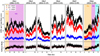 |
Fig. 1. XMM-Newton/EPIC-pn light curves (red points: 0.3−2 keV; blue points: 2−10 keV; black points: 0.3−10 keV) of NGC 3227 (top panel) and softness ratio curves between the count rates in 0.3−2 keV and 2−10 keV bands (Soft0.3 − 2 keV/Hard2 − 10 keV; bottom panel) with the time bin of 100 s. The red horizontal dashed line in the bottom panel is the average softness ratio of all the six observations. According to the difference between the softness ratio of each observation (black points in the bottom panel) and the average softness ratio (horizontal dashed line in red), Obs1 is divided into two slices that are S1a (orange region of the first column) and S1b (violet region of the first column), and Obs6 is divided into three slices that are S6a (orange region of the last column), S6b (violet region of the last column), and S6c (cyan region of the last column). |
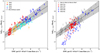 |
Fig. 2. Correlation between the softness ratio (the ratio of count rates between 0.3−2 and 2−10 keV bands), and 0.3−10 keV count rate, for Obs2 to Obs5 (left panel), and for Obs1 and Obs6 (right panel). In both left and right panels, the black solid line is the best-fit linear model of y = (0.06 ± 0.01)x + (1.54 ± 0.13) for Obs2 to Obs5. The shaded grey region is the associated 1σ uncertainty. |
Obs1. This observation was considered to be in an unobscured state by Markowitz et al. (2009). However, compared with the average softness ratio of the six observations (see the dashed red line in the bottom panel of Fig. 1), a significant spectral hardening (softness ratio below the average value) occurred in the beginning of this observation (see the bottom panel of the first column in Fig. 1), which might indicate the existence of an obscuration event. After this spectral hardening period, the softness ratio of Obs1 returns to the average value, which might indicate that this obscuration event has disappeared. These phenomena mean that these two periods of Obs1 should be analyzed separately. According to the difference between the softness ratio of Obs1 and the average softness ratio of the six observations, Obs1 is subdivided into the following two slices: S1a and S1b (see the first column in Fig. 1). S1b is consistent with being in an unobscured state as it follows the correlation of Obs2 to Obs5 (see the right panel of Fig. 2). However, S1a has a harder spectrum that is similar to S6a and S6b (see the right panel of Fig. 2), and it might be in an obscured state (however, this was not reported in previous works).
Obs2 to Obs5. According to Turner et al. (2018), Obs2 to Obs5 are in unobscured states, which show a linear correlation between the softness ratio (0.3−1/1−10 keV) and 0.3−10 keV count rate. We confirm this linear correlation for these observations (softness ratio is calculated between the 0.3−2 and 2−10 keV bands in this work) in the left panel of Fig. 2. It is worth noting that although Obs2 and Obs3 show a spectral hardening during some periods, these periods still follow the correlation of unobscured states (see the left panel of Fig. 2). Therefore, these periods might not be in obscured states.
Obs6. Turner et al. (2018) had observed a rapid obscuration event in Obs6. To restudy this obscuration event using a broadband SED model and the pion model in SPEX, we followed Turner et al. (2018) to subdivide Obs6 into three slices: S6a, S6b, and S6c (see Fig. 1). S6c shows an unobscured state as it follows the correlation of Obs2 to Obs5 (see the right panel of Fig. 2). However, S6a and S6b deviate from the correlation of Obs2 to Obs5 (see the right panel of Fig. 2); therefore, they might reside in obscured states.
Next, we carried out a detailed spectral analysis for these observational data. We began our spectral modeling by using a broadband SED model from the NIR to the hard X-ray bands for NGC 3227. We refer to our Paper I for the full details on this SED model and we only give a brief introduction here. The main spectral components that are used in this work are as follows.
1. The intrinsic broadband SED (see details in Paper I), which is composed of a disk blackbody component (dbb), a warm Comptonized disk component (comt) from the optical to the soft X-ray band, an X-ray power-law component (pow), and a neutral reflection component (refl) in the hard X-ray energy band. For the pow of NGC 3227, we used 309 keV (Turner et al. 2018) as the high-energy exponential cut-off and 13.6 eV as the low-energy exponential cut-off.
2. The obscurer components, which heavily absorb the X-ray spectrum. We used the pion model in SPEX to fit their absorption features in the spectrum.
3. The warm absorber (WA) components, which produce absorption features in soft X-rays. We also used the pion model to fit these absorption features.
4. The Galactic X-ray absorption, which was taken into account by the hot model in SPEX with the hydrogen column density NH = 2.07 × 1020 cm−2 (Murphy et al. 1996).
Obs2 to Obs5, S1b, and S6c are in unobscured states, so we will fit their spectra using the spectral components 1, 3, and 4. S1a, S6a, and S6b are in obscured states, so their spectra will be fitted with spectral components 1–4. In the next subsection, we present the details of the spectral analysis for spectral components 1, 2, and 3.
3.1. The intrinsic broadband SED
For the archival data, only the OM UVW1 filter data is available for all the six observations, so the parameters of the dbb component might not be well constrained for the fit. Moreover, we do not expect a strong variability in the shape of the emission from the outer disc on short timescales. It is also common for the variability of the flux in long wavelengths to be significantly smaller than that of the X-ray band. Therefore, we assume that the shape of the dbb component of each archival observation is similar to that of the 2019 observation which has optical and UV observational data to constrain the dbb component (see Paper I); that is to say, we fixed the maximum temperature Tmax of the dbb component of the archival data to the 10 eV of the 2019 observation (see Paper I) and scaled the dbb normalization of the archival observations according to the normalization of the 2019 observation (the scale factor of each archival observation is the OM UVW1 flux ratio between the 2019 observation and each archival observation). For the comt component, its normalization was free in the fit and the following parameters were fixed to those of the 2019 observation (see details in Paper I): seed photon temperature Tseed = 10 eV, electron temperature Te = 60 eV, and optical depth τ = 30. The dbb and comt components mainly dominate in the energy band below 0.5 keV (see Paper I), so fixing the shapes of these two components might bring uncertainties to the parameter estimates for the WAs. Even so, the normalizations of these two components, which are free in the fits, are still the main factors to affect the fitting result. For each slice in an obscured state (S1a, S6a, and S6b), we assumed that it has the same intrinsic broadband SED as the unobscured slice in the same observation (S1b, S6c, and S6c, respectively). Therefore, we fixed the parameters of dbb, comt, pow, and refl components of S1a to those of S1b in the fit. Similarly, these parameters of S6a and S6b were fixed to those of S6c. For the refl component, the scaling factor of the reflected spectrum (s) was free in the fit, the incident power-law normalization and photon index were coupled to those of the pow component. We summarize the best-fit parameters of the intrinsic broadband SED in Table 2 (discussed in Sect. 4.1).
Best-fit parameters of the intrinsic broadband SED.
3.2. Warm absorber components
The hydrogen column density (NH), outflow velocity (vout), and turbulent velocity (σv) of the WAs are not well constrained simultaneously for the spectrum with low S/N and these parameters might not vary significantly between different observations. Therefore, we fixed these parameters of Obs1–Obs4 and Obs6 to the best-fit results of Obs5 (see Table 3), because Obs5 has the highest S/N. Therefore, for Obs1–Obs4 and Obs6, only ξ was free in the fit (see Table 3). Actually, NH, vout, and σv are not expected to be constant, so our assumption will bring extra uncertainties to the parameter estimates. However, NH, vout, and σv might not vary significantly on short timescales compared with ξ, so a significant impact on the fitting results with these parameters fixed might not be expected. For simplicity, we assumed that the WAs fully cover the X-ray source (covering factor Cf = 1) and have solar abundances (Lodders et al. 2009). The best-fit results of the WAs are discussed in Sect. 4.2.
Best-fit parameters of the four WAs (WA1, WA2, WA3, WA4) for Obs1 to Obs6: hydrogen column density (NH), ionization parameter (ξ), outflow velocity (vout), and turbulent velocity (σv).
3.3. Obscurer components
Parameters vout and σv of the obscurer components were difficult to constrain owing to the lack of well defined and strong absorption lines. We verified that changing their values had little impact on other parameters. Therefore, we fixed vout and σv of the obscurer components to their default values (vout = 0 km s−1 and σv = 100 km s−1). With that, the obscurer components, NH, ξ, and Cf are free in the fit. We will discuss the best-fit results of obscurer components in Sect. 4.3.
4. Results and discussion
4.1. Intrinsic broadband SED
The broadband SED model provides a good description for the observational data (see Table 2 and Fig. 3, where Obs5 is given as an example). Compared with other observations or slices, Obs1 S1b and Obs2 have relatively worse fitting results (see Table 3); this is mainly due to the uncertainties in the intercalibration between XMM-Newton and NuSTAR. The intrinsic unabsorbed broadband SEDs of Obs1 to Obs6 are shown in Fig. 4 and their best-fit parameters are listed in Table 2. The intrinsic broadband SED of NGC 3227 shows a significant variability at energies ≥0.03 keV, especially in the X-ray band (see Fig. 4). According to the Spearman rank method, there is a positive correlation between the photon index of the pow (Γ; see Table 2) and the intrinsic 2−10 keV luminosity (L2 − 10 keV; see Table 2), where the correlation coefficients rs = 0.94 and the associated p-values ps = 0.005, showing a “softer-when-brighter” behavior. This behavior has been observed in many Seyfert galaxies (e.g., Markowitz & Edelson 2004; Ponti et al. 2006; Sobolewska & Papadakis 2009; Soldi et al. 2014). Peretz & Behar (2018) also found a softer-when-brighter variability behavior in NGC 3227, which might be driven by varying absorption rather than by the intrinsic variability of the central source. The averaged ionizing luminosity over 1−1000 Ryd is around 1.9 × 1043 erg s−1 (see Table 2), which is two times larger than the results of Beuchert et al. (2015) and Turner et al. (2018). This might be due to the different SED model in the UV and soft X-ray bands. The averaged full-band bolometric luminosity (Lbol) is about 4.6 × 1043 erg s−1 (see Table 2), which is 1.5 times smaller than the result of Woo & Urry (2002) based on the flux integration method. According to the reverberation mapping method, the black hole mass (MBH) of NGC 3227 is 5.96 × 10⁶ M⊙ for NGC 3227 (Bentz & Katz 2015). The Eddington luminosity (LEdd) of NGC 3227 is 7.45 × 1044 erg s−1, which is calculated by LEdd = 1.25 × 1038 × (MBH/M⊙) (Rybicki & Lightman 1979). Therefore, the averaged Eddington ratio of NGC 3227 is about 6%.
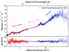 |
Fig. 3. Observational data (colored data points) with the best-fit broadband SED model in the X-ray band (black solid curve) for Obs5 (top panel). Residuals of the best-fit model (“D” is the observational data and “M” is the best-fit model) for Obs5 (bottom panel). Obs5 is given as an example (other observations have similar fitting results). |
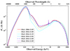 |
Fig. 4. Intrinsic unabsorbed broadband SEDs of Obs1–Obs6. |
4.2. Warm absorber components
At least four WA components (see Table 3) were required to improve the fitting result (ΔC ∼ 100 for adding WA1, ΔC ∼ 80 for adding WA2, ΔC ∼ 80 for adding WA3, ΔC ∼ 500 for adding WA4). We added another component (a fifth component), but it did not improve the fitting result (ΔC ∼ 2). Our result is not consistent with that in Turner et al. (2018), which detected three WA components. This might be due to the different SED model and photoionization models between our respective works. The best-fit model shows some weak residual emission features in the 0.5−0.6 keV band (see Fig. 3) caused by the oxygen line emission from distant regions, similarly to NGC 5548 (Mao et al. 2018). The quality of our spectrum is not equipped for a detailed modeling of these emission lines, and they are too weak to affect our modeling of the absorbing wind components. Thus, we do not discuss them further.
4.2.1. Parameters of the warm absorbers
The logarithm of the ionization parameter (in units of erg cm s−1) for each WA component is around 3.0 for WA1, 2.5 for WA2, 2.0 for WA3, and −1.0 for WA4 (see Table 3). WA2, WA3, and WA4 have a similar column density around 1021 cm−2, while WA1 has a much higher value near 1022 cm−2 (see Table 3). In Paper I, we adopt a de-ionization scenario for the WAs and simultaneous fitted the spectra of the archival unobscured observation taken on December 5, 2016 and the new obscured observations taken in 2019. In this work, we fit the spectra taken on 2016 December 05 alone. Therefore, some different results between Paper I and Paper II can be expected because of the differences in the spectral modeling. The X-ray transmission of each WA component in our line of sight to the central region is shown in the top panel of Fig. 5. We can see that WA1 mainly absorbs the continuum radiation between 0.8 and 10 keV. Furthermore, WA2 and WA3 produce absorption features between 0.7 and 5 keV, whereas WA4 heavily absorbs the continuum below 5 keV. From WA1 to WA4, the outflow velocity gradually decreases from ∼1300 to ∼100 km s−1 (see Table 3), which shows a positive correlation with the ionization parameter. This correlation is consistent with the results for AGN samples (Tombesi et al. 2013; Laha et al. 2014). These previous studies indicated that this correlation cannot be explained by the radiatively driven or magneto hydrodynamically driven outflowing mechanism (Tombesi et al. 2013; Laha et al. 2014), and it might be explained by the equilibrium between the radiation pressure on WAs and the drag pressure from the ambient circumnuclear medium (see details in Wang et al., in prep.).
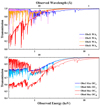 |
Fig. 5. Transmission spectra of the four WAs of Obs5 (WA1, WA2, WA3, WA4 (top panel; Obs5 is given as an example) and obscurer components of S6a, S6b, and S1a (bottom panel). OCL is the low-ionization obscurer component, while OCH is the high-ionization obscurer component. |
4.2.2. Radial location of the warm absorbers
We used three methods to estimate the upper or lower limit of the locations of the various WA components. First, we assumed that the thickness (Δr) of the WA cloud does not exceed its distance (r) to the SMBH (Krolik & Kriss 2001; Blustin et al. 2005). As NH ≈ nHCvΔr, so the upper limit of the distance rmax ≈ Δr ≈ NH/(nHCv), where Cv is the volume filling factor. Combined with Eq. (1), rmax can be estimated by
 (2)
(2)
Assuming that the total outflow momentum of the WA cloud is equal to the momentum of the absorbed radiation (Pabs) plus the momentum of the ionizing luminosity being scattered (Pscat), Cv can be calculated as follows (Blustin et al. 2005; Grafton-Waters et al. 2020):
 (3)
(3)
Here, Ṗabs is given by
 (4)
(4)
where Labs is the absorbed luminosity, and Ṗscat is calculated by
 (5)
(5)
where τT is the optical depth for Thomson scattering, and σT is the Thomson scattering cross-section. We use the ionizing luminosity of Obs5 to estimate the distance as the WAs parameters are mainly from the spectral fitting of Obs5. The estimated upper limit (rmax in Eq. (2)) of the radial location of each WA component is summarized in Table 4, which is 0.007 pc for WA1, 0.24 pc for WA2, 0.71 pc for WA3, and 265 pc for WA4.
Estimated distances (r) of the four WAs (WA1, WA2, WA3, and WA4) of NGC 3227.
The second method is based on the assumption that the outflow velocities of winds are larger than or equal to their escape velocities  (Blustin et al. 2005), then we can obtain the lower limit of r via:
 (6)
(6)
where G is the gravitational constant. The lower limit of the radial location of each WA component is estimated to be 0.03 pc for WA1, 0.2 pc for WA2, 0.3 pc for WA3, and 4 pc for WA4 (see Table 4).
The third method for estimating the radial location of WAs is based on the recombination timescale. Following Bottorff et al. (2000), the recombination timescale of the ion Xi is defined as
![Mathematical equation: $$ \begin{aligned} t_{\mathrm{rec}}(X_{\rm i}) = \bigg (\alpha _{\mathrm{r}}(X_{\rm i})n_{\rm e} \bigg [\frac{f(X_{i+1})}{f(X_{\rm i})}-\frac{\alpha _{\mathrm{r}}(X_{i-1})}{\alpha _{\mathrm{r}}(X_{\rm i})}\bigg ]\bigg )^{-1}, \end{aligned} $$](/articles/aa/full_html/2022/01/aa41599-21/aa41599-21-eq30.gif) (7)
(7)
where αr(Xi) is the recombination coefficient (recombination rate from the ion Xi + 1 to Xi), ne is the electron number density of the absorbing gas, and f(Xi) is the fraction of ion Xi. We select the ions that contribute significantly to the spectral fit for each WA component as the indicators of this component. Some of these parameters can be obtained from SPEX code (Mao & Kaastra 2016): αr(Xi) and αr(Xi − 1) come from atomic physics, and f(Xi) and f(Xi + 1) are estimated from the ionization balance. Then we can obtain ntrec (see Table 4). The trec of each WA component can be estimated by the variation timescale of the ionization parameters between different observations (e.g., Ebrero et al. 2016b). For WA1, the ionization parameter shows a significant variation between Obs2 and Obs3, so its trec might be lower than the time interval between Obs2 and Obs3 (16 days). For WA2, there is a significant change for the ionization parameter between Obs3 and Obs5, so its trec might be smaller than the time interval between Obs3 and Obs5 (10 days). For both WA3 and WA4, Obs3, and Obs4 have a significantly different ionization parameter, which indicates that their values for trec might be smaller than the time interval between Obs3 and Obs4 (6 days). However, we cannot make a clear conclusion about the lower limits of the trec for these WA components because of the low number of observations. We list the trec of each WA component in Table 4. According to trec, ntrec, and Eq. (1) (we also use the ionizing luminosity of Obs5 here), the radial distance is estimated to be ≲0.16 pc for WA1, ≲0.3 pc for WA2, ≲0.6 pc for WA3, ≲13 pc for WA4 (see Table 4). These estimates are consistent with the results obtained by Eqs. (2) and (6) (see Table 4 and Fig. 6).
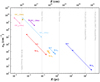 |
Fig. 6. Distances of the four WAs (WA1, WA2, WA3, WA4) and four obscurer components from the center of NGC 3227. Here, OCL is the low-ionization obscurer component and OCH is the high-ionization obscurer component. The symbols “◂” for the WAs represent the upper limits of the distance estimated by the assumption that the thickness of the WA cloud does not exceed its distance to the SMBH (see Eq. (2)). The symbols “↦” for the WAs represent the lower limits of the distance estimated by the assumption that the outflow velocities of winds are larger than or equal to their escape velocities (see Eq. (6)). The symbols “◃” for the WAs represent the upper limits of the distance estimated by the upper limits of the recombination timescale (see Eq. (7)). The symbols “▸” and “◂” for the obscurer components represent the lower and upper limits of the distance estimated by the range of the crossing time (see Eq. (10)). The radial location of the optical BLR of NGC 3227 is estimated by the time lag between the Hβ line and continuum at 5100 Å (Denney et al. 2009). The inner radii of the torus are estimated by the dust sublimation radius (see Eq. (8)) and its outer radii are estimated by Rout = Y × Rin (Y = 17 for NGC 3227; Alonso-Herrero et al. 2011). The location of the NLR is estimated by the optical [O III] λ5007 image (Mundell et al. 1995; Schmitt & Kinney 1996). |
The radial location of the optical BLR of NGC 3227 is estimated to be around 0.0032 pc from the time lag between the Hβ line and continuum at 5100 Å (Denney et al. 2009). The optical [O III] λ5007 image indicates that the narrow line region (NLR) of NGC 3227 can extend to ∼100 pc (Schmitt & Kinney 1996), even to ∼500 pc (Mundell et al. 1995). According to Nenkova et al. (2008a), the inner radius of the torus can be estimated by
 (8)
(8)
with a dust temperature of Td = 1500 K. If Lbol = 4.6 × 1043 erg s−1 (see Sect. 4.1), Rin is about 0.09 pc. The outer radius can be estimated by Rout = Y × Rin. Using the clumpy model (Nenkova et al. 2002, 2008a,b), Alonso-Herrero et al. (2011) estimated that the Y of NGC 3227 is about 17, so Rout is around 1.46 pc. The distance estimates for the BLR, torus, NLR, and each WA component of NGC 3227 are shown in Fig. 6.
As Fig. 6 shows, WA1 lies between the outer region of the BLR and the inner region of torus; WA2 and WA3 might be in the torus; WA4 likely resides between the outer torus and the NLR, and it is the one that is farthest away from the AGN compared with other WAs, which might explain the lowest ionization parameter of this component (see details in Sect. 4.2.1 and Table 3). For the distance estimation of WA1, the first and second methods give inconsistent results, which might be due to the following reasons: (1) these two methods use different assumptions, which can be expected to have different results; (2) we did not consider the possible contribution from the momentum associated with other processes (e.g., magnetic field), which might not be negligible for WA1 and might lead to an underestimation for Cv (see Eq. (3)) and rmax (see Eq. (2)).
4.3. Obscurer components
According to the softness ratio (see Sect. 3), S6a, S6b, and S1a seem to be in obscured states, which may be caused by the clouds (obscurer components) crossing the line of sight. Then we make detailed spectral modeling to check whether the obscurer components are required to explain the significant spectral variation in these slices. Firstly, we fixed the parameters of the intrinsic SED and WAs of S1a to those of S1b that is in the unobscured state because we do not expect strong variabilities in the SED shape and WAs parameters on small time scales between S1a and S1b. However, the absorption features in the soft X-rays cannot be explained by WAs alone. Therefore, we add an obscurer component, which greatly improves the fitting result (ΔC ∼ 785). Similarly, we firstly fixed the intrinsic SED and WAs parameters of S6b to those of S6c that is in the unobscured state. One obscurer component is also required to improve the fitting result with ΔC ∼ 1218. Adding a second obscurer component cannot improve the fitting result of both S1a and S6b. For S6a, we firstly fixed its intrinsic SED and WAs parameters to those of S6c, which cannot explain the observational data well. We verified that two obscurer components are required to improve the fitting result: ΔC ∼ 13 582 for adding one obscurer component and ΔC ∼ 31 for adding a second obscurer component.
4.3.1. Parameters of the obscurer components
The spectral analysis indicates that S6a has two obscurer components: a high-ionization component ( ; S6a OCH) with Cf of
  and a low-ionization component (
 ; S6a OCL) with Cf of 0.46 ± 0.03. S6b and S1a only have one low-ionization obscurer component, respectively: log ξ = 1.89 ± 0.11 for S6b OCL with Cf of 0.35 ± 0.03 and
  for S1a OCL with Cf of 0.21 ± 0.02 (see Table 5). The low-ionization obscurer component (OCL) has a lower column density (∼1022 cm−2) than the high-ionization obscurer component (OCH; NH ∼ 1023 cm−2) (see Table 5). S6a OCL has a larger covering factor than S6a OCH, considering 1σ level uncertainties. Our result for S6a is not consistent with that in Turner et al. (2018), which only found one obscurer component with NH ∼ 1022 cm−2, log ξ ∼ 2, and Cf ∼ 60%. It might be due to the different SED model and different spectral modeling process. The X-ray transmission of each obscurer component in our line of sight to NGC 3227 is shown in Fig. 5. The OCL components can produce absorption features at energies lower than 6 keV, and the OCH component mainly absorbs the continuum at energies higher than 0.5 keV.
Best-fit parameters of the obscurer components for S6a, S6b, and S1a: hydrogen column density (NH), ionization parameter (ξ), covering factor (Cf).
4.3.2. Radial location of the obscurer components
As we mention in Sect. 3.3, we cannot constrain the outflow velocities of the obscurer components, so we cannot estimate the distance of the obscurer components using the same methods as for the WAs. Here, we estimate the distance of the obscurer components based on the crossing time of the obscuring cloud. For simplicity, we assume that an obscuring cloud moves around the central black hole (MBH) in a circular orbit of radius R, so that the keplerian velocity of the obscuring cloud crossing the line of sight is  . Assuming a spherical geometry for the obscuring cloud, its diameter is D ∼ NH/nH and the size of this cloud crossing the line of sight is approximately equal to D, so that vcloud can also be given by vcloud = D/tcross = NH/(nHtcross), where tcross is the crossing time of the obscuring cloud. Therefore, we can obtain a relation for nH:
 (9)
(9)
Following Lamer et al. (2003), we combine Eqs. (1) and (9) to obtain R:
 (10)
(10)
where M7 = MBH/107 M⊙, L42 = Lion/1042 erg s−1, tdays is tcross in days, and N22 = NH/1022 cm−2.
On the one hand, Obs5 is in an unobscured state, which indicates that OCH and OCL of S6a do not start to cross the line of sight during the observational time of Obs5. One the other hand, OCH of S6a disappears in the observational time of S6b. Therefore, tcross of OCH should be larger than the exposure time of S6a (39 ks) and smaller than the time interval between Obs5 and Obs6 (309 ks). If we assume that S6a and S6b have different OCL components, tcross of S6a OCL should be also between 39 and 309 ks (similar to the case of S6a OCH), and tcross of S6b OCL should be comparable to the exposure time of S6b (20 ks). Similarly, tcross of S1a OCL should be larger than the exposure time of S1a (20 ks), and smaller than the time interval (372 days) between Obs1 and an unobscured observation taken in November 2005 (see Fig. A.12 of Markowitz et al. 2014). The estimated crossing time of each obscurer component is summarized in Table 6. Then, we can use Eq. (10) to constrain the location of each obscurer component, which is shown in Table 6 and Fig. 6. These obscurer components are estimated to be located within the BLR, which is consistent with the results in previous works (Lamer et al. 2003; Beuchert et al. 2015; Turner et al. 2018).
Crossing time (tcross) and distances (R) of the obscurer components for S6a, S6b, and S1a.
The obscurers of NGC 3227 are closer to the SMBH than the WAs and also have a significantly larger hydrogen or electron number density than the WAs (see Fig. 6). Besides that, the obscurers usually appear on a short timescale while WAs can exist for a long time, and the appearance of the obscurers mainly affects the ionization state of the WAs on the short timescale. These results indicate that the obscurers and WA outflows might have different origins. For example, obscurers might be triggered by the collapse of inner BLR clouds (Kriss et al. 2019a,b; Devereux 2021), while WA outflows might be formed by the outflowing of the clouds between outer BLR and NLR under the drive of the radiation pressure (e.g., Proga & Kallman 2004), magnetic forces (e.g., Blandford & Payne 1982; Konigl & Kartje 1994; Fukumura et al. 2010), or thermal pressure (e.g., Begelman et al. 1983; Krolik & Kriss 1995; Mizumoto et al. 2019). However, we cannot get a solid conclusion in this work, which might require more high-quality data to investigate.
5. Summary and conclusions
The relationship between WA outflows of AGN and nuclear obscuration activities remains unclear. We find that NGC 3227 is a suitable target for the study of the properties of both WAs and obscurers, which might help us understand their correlation. To investigate the WA components of NGC 3227 in detail, we used a broadband SED model (Paper I) and the photoionization model in SPEX software to fit the unobscured spectra of the archival and previously published XMM-Newton and NuSTAR observations taken in 2006 and 2016. Based on the broadband SED and WAs parameters, we also study the X-ray obscuration events in the archival observations.
We detect four ionization phases for the WAs in NGC 3227 using the unobscured observations: log ξ (erg cm s−1) ∼ −1.0, 2.0, 2.5, 3.0. The highest-ionization WA component has a much higher hydrogen column density (NH ∼ 1022 cm−2) than the other three WA components (NH ∼ 1021 cm−2). The outflow velocities of these WA components range from ∼100 to ∼1300 km s−1, and show a positive correlation with the ionization parameter. Our estimates of the radial location of these WA components indicate that the WAs of NGC 3227 might reside over radii ranging from the BLR to the torus – even up to the NLR.
We find an obscuration event in 2006, which was missed by previous studies. One obscurer component is required for this 2006 obscuration event. For the previously published obscuration event in 2016, we detect two obscurer components. A high-ionization obscurer component ( ; covering factor
  ) only appears in the 2016 observation, which has a column density around 1023 cm−2, while both the 2006 and 2016 observations have a low-ionization obscurer component (log ξ ∼ 1.0 − 1.9; Cf ∼ 0.2 − 0.5), which has a lower column density (∼1022 cm−2) than the high-ionization obscurer component. Assuming that the variations of flux is caused by the transverse motion of obscurers across the line of sight, we estimate the locations of the obscurers to be within the BLR.
The obscurers of NGC 3227 are closer to the SMBH than the WAs and have a significantly larger hydrogen or electron number density than the WAs. In addition, the obscurers usually appear on a short timescale while the WAs have the capacity to exist for a long time. These proofs indicate that the obscurers and WAs of NGC 3227 might have different origins.
The redshift of NGC 3227 is obtained from the NASA/IPAC Extragalactic Database (NED: https://ned.ipac.caltech.edu/ ). The NED is funded by the National Aeronautics and Space Administration and operated by the California Institute of Technology.
See https://www.cosmos.esa.int/web/xmm-newton/sas-threads for details.
Acknowledgments
We thank the referee for helpful comments that improved this paper. This research has made use of the NASA/IPAC Extragalactic Database (NED), which is funded by the National Aeronautics and Space Administration and operated by the California Institute of Technology. YJW gratefully acknowledges the financial support from the China Scholarship Council. YJW and YQX acknowledge support from NSFC-12025303, 11890693, 11421303, the CAS Frontier Science Key Research Program (QYZDJ-SSW-SLH006), the K.C. Wong Education Foundation, and the science research grants from the China Manned Space Project with NO. CMS-CSST-2021-A06. SRON is supported financially by NWO, the Netherlands Organization for Scientific Research. JM acknowledges the support from STFC (UK) through the University of Strathclyde UK APAP network grant ST/R000743/1. GP acknowledges funding from the European Research Council (ERC) under the European Union’s Horizon 2020 research and innovation programme (grant agreement No 865637). E.B. is funded by a Center of Excellence of THE ISRAEL SCIENCE FOUNDATION (grant No. 2752/19). SB acknowledges financial support from ASI under grants ASI-INAF I/037/12/0 and n. 2017-14-H.O., and from PRIN MIUR project “Black Hole winds and the Baryon Life Cycle of Galaxies: the stone-guest at the galaxy evolution supper”, contract no. 2017PH3WAT. BDM acknowledges support via Ramón y Cajal Fellowship RYC2018-025950-I. SGW acknowledges the support of a PhD studentship awarded by the UK Science & Technology Facilities Council (STFC). DJW acknowledges support from STFC in the form of an Ernest Rutherford fellowship. P.O.P. acknowledges financial support from the CNES french agency and the PNHE high energy national program of CNRS.
References
- Alonso-Herrero, A., Ramos Almeida, C., Mason, R., et al. 2011, ApJ, 736, 82 [NASA ADS] [CrossRef] [Google Scholar]
- Begelman, M. C., McKee, C. F., & Shields, G. A. 1983, ApJ, 271, 70 [CrossRef] [Google Scholar]
- Bentz, M. C., & Katz, S. 2015, PASP, 127, 67 [Google Scholar]
- Beuchert, T., Markowitz, A. G., Krauß, F., et al. 2015, A&A, 584, A82 [NASA ADS] [CrossRef] [EDP Sciences] [Google Scholar]
- Beuchert, T., Markowitz, A. G., Dauser, T., et al. 2017, A&A, 603, A50 [NASA ADS] [CrossRef] [EDP Sciences] [Google Scholar]
- Blandford, R. D., & Payne, D. G. 1982, MNRAS, 199, 883 [CrossRef] [Google Scholar]
- Blustin, A. J., Page, M. J., Fuerst, S. V., Branduardi-Raymont, G., & Ashton, C. E. 2005, A&A, 431, 111 [NASA ADS] [CrossRef] [EDP Sciences] [Google Scholar]
- Bottorff, M. C., Korista, K. T., & Shlosman, I. 2000, ApJ, 537, 134 [NASA ADS] [CrossRef] [Google Scholar]
- Crenshaw, D. M., Kraemer, S. B., & George, I. M. 2003, ARA&A, 41, 117 [NASA ADS] [CrossRef] [Google Scholar]
- De Marco, B., Adhikari, T. P., Ponti, G., et al. 2020, A&A, 634, A65 [NASA ADS] [CrossRef] [EDP Sciences] [Google Scholar]
- Denney, K. D., Peterson, B. M., Pogge, R. W., et al. 2009, ApJ, 704, L80 [NASA ADS] [CrossRef] [Google Scholar]
- Devereux, N. 2021, MNRAS, 500, 786 [Google Scholar]
- Ebrero, J., Kaastra, J. S., Kriss, G. A., de Vries, C. P., & Costantini, E. 2013, MNRAS, 435, 3028 [NASA ADS] [CrossRef] [Google Scholar]
- Ebrero, J., Kriss, G. A., Kaastra, J. S., & Ely, J. C. 2016a, A&A, 586, A72 [NASA ADS] [CrossRef] [EDP Sciences] [Google Scholar]
- Ebrero, J., Kaastra, J. S., Kriss, G. A., et al. 2016b, A&A, 587, A129 [NASA ADS] [CrossRef] [EDP Sciences] [Google Scholar]
- Elvis, M. 2000, ApJ, 545, 63 [NASA ADS] [CrossRef] [Google Scholar]
- Fukumura, K., Kazanas, D., Contopoulos, I., & Behar, E. 2010, ApJ, 715, 636 [NASA ADS] [CrossRef] [Google Scholar]
- Gibson, R. R., Jiang, L., Brandt, W. N., et al. 2009, ApJ, 692, 758 [Google Scholar]
- Grafton-Waters, S., Branduardi-Raymont, G., Mehdipour, M., et al. 2020, A&A, 633, A62 [EDP Sciences] [Google Scholar]
- Halpern, J. P. 1984, ApJ, 281, 90 [NASA ADS] [CrossRef] [Google Scholar]
- Kaastra, J. S. 2017, A&A, 605, A51 [NASA ADS] [CrossRef] [EDP Sciences] [Google Scholar]
- Kaastra, J. S., Mewe, R., & Nieuwenhuijzen, H. 1996, UV and X-ray Spectroscopy of Astrophysical and Laboratory Plasmas, 411 [Google Scholar]
- Kaastra, J. S., Mewe, R., Liedahl, D. A., Komossa, S., & Brinkman, A. C. 2000, A&A, 354, L83 [NASA ADS] [Google Scholar]
- Kaastra, J. S., Kriss, G. A., Cappi, M., et al. 2014, Science, 345, 64 [Google Scholar]
- Kaastra, J. S., Mehdipour, M., Behar, E., et al. 2018, A&A, 619, A112 [NASA ADS] [CrossRef] [EDP Sciences] [Google Scholar]
- Kaastra, J. S., Raassen, A. J. J., de Plaa, J., & Gu, L. 2020, https://doi.org/10.5281/zenodo.4384188 [Google Scholar]
- Kara, E., Mehdipour, M., Kriss, G. A., et al. 2021, ApJ, 922, 151 [NASA ADS] [CrossRef] [Google Scholar]
- King, A., & Pounds, K. 2015, ARA&A, 53, 115 [NASA ADS] [CrossRef] [Google Scholar]
- Komossa, S., & Fink, H. 1997, A&A, 327, 483 [NASA ADS] [Google Scholar]
- Konigl, A., & Kartje, J. F. 1994, ApJ, 434, 446 [NASA ADS] [CrossRef] [Google Scholar]
- Kriss, G. A., Mehdipour, M., Kaastra, J. S., et al. 2019a, A&A, 621, A12 [NASA ADS] [CrossRef] [EDP Sciences] [Google Scholar]
- Kriss, G. A., De Rosa, G., Ely, J., et al. 2019b, ApJ, 881, 153 [NASA ADS] [CrossRef] [Google Scholar]
- Krolik, J. H., & Kriss, G. A. 1995, ApJ, 447, 512 [NASA ADS] [CrossRef] [Google Scholar]
- Krolik, J. H., & Kriss, G. A. 2001, ApJ, 561, 684 [CrossRef] [Google Scholar]
- Krongold, Y., Nicastro, F., Elvis, M., et al. 2007, ApJ, 659, 1022 [NASA ADS] [CrossRef] [Google Scholar]
- Laha, S., Guainazzi, M., Dewangan, G. C., Chakravorty, S., & Kembhavi, A. K. 2014, MNRAS, 441, 2613 [NASA ADS] [CrossRef] [Google Scholar]
- Laha, S., Reynolds, C. S., Reeves, J., et al. 2021, Nat. Astron., 5, 13 [NASA ADS] [CrossRef] [Google Scholar]
- Lamer, G., Uttley, P., & McHardy, I. M. 2003, MNRAS, 342, L41 [NASA ADS] [CrossRef] [Google Scholar]
- Lodders, K., Palme, H., & Gail, H. P. 2009, Landolt Börnstein, 4B, 712 [Google Scholar]
- Lohfink, A. M., Reynolds, C. S., Mushotzky, R. F., & Wilms, J. 2012, ApJ, 749, L31 [NASA ADS] [CrossRef] [Google Scholar]
- Longinotti, A. L., Krongold, Y., Kriss, G. A., et al. 2013, ApJ, 766, 104 [NASA ADS] [CrossRef] [Google Scholar]
- Mao, J., & Kaastra, J. 2016, A&A, 587, A84 [NASA ADS] [CrossRef] [EDP Sciences] [Google Scholar]
- Mao, J., Kaastra, J. S., Mehdipour, M., et al. 2018, A&A, 612, A18 [NASA ADS] [CrossRef] [EDP Sciences] [Google Scholar]
- Markowitz, A., & Edelson, R. 2004, ApJ, 617, 939 [NASA ADS] [CrossRef] [Google Scholar]
- Markowitz, A., Reeves, J. N., George, I. M., et al. 2009, ApJ, 691, 922 [NASA ADS] [CrossRef] [Google Scholar]
- Markowitz, A. G., Krumpe, M., & Nikutta, R. 2014, MNRAS, 439, 1403 [Google Scholar]
- Mehdipour, M., Kaastra, J. S., & Kallman, T. 2016, A&A, 596, A65 [NASA ADS] [CrossRef] [EDP Sciences] [Google Scholar]
- Mehdipour, M., Kaastra, J. S., Kriss, G. A., et al. 2017, A&A, 607, A28 [NASA ADS] [CrossRef] [EDP Sciences] [Google Scholar]
- Mehdipour, M., Kriss, G. A., Kaastra, J. S., et al. 2021, A&A, 652, A150 [NASA ADS] [CrossRef] [EDP Sciences] [Google Scholar]
- Mizumoto, M., Done, C., Tomaru, R., & Edwards, I. 2019, MNRAS, 489, 1152 [NASA ADS] [CrossRef] [Google Scholar]
- Mundell, C. G., Holloway, A. J., Pedlar, A., et al. 1995, MNRAS, 275, 67 [NASA ADS] [Google Scholar]
- Murphy, E. M., Lockman, F. J., Laor, A., & Elvis, M. 1996, ApJS, 105, 369 [NASA ADS] [CrossRef] [Google Scholar]
- Murray, N., Chiang, J., Grossman, S. A., & Voit, G. M. 1995, ApJ, 451, 498 [NASA ADS] [CrossRef] [Google Scholar]
- Nenkova, M., Ivezić, Ž., & Elitzur, M. 2002, ApJ, 570, L9 [NASA ADS] [CrossRef] [Google Scholar]
- Nenkova, M., Sirocky, M. M., Nikutta, R., Ivezić, Ž., & Elitzur, M. 2008a, ApJ, 685, 160 [Google Scholar]
- Nenkova, M., Sirocky, M. M., Ivezić, Ž., & Elitzur, M. 2008b, ApJ, 685, 147 [Google Scholar]
- Newman, J., Tsuruta, S., Liebmann, A. C., Kunieda, H., & Haba, Y. 2021, ApJ, 907, 45 [NASA ADS] [CrossRef] [Google Scholar]
- Parker, M. L., Longinotti, A. L., Schartel, N., et al. 2019, MNRAS, 490, 683 [NASA ADS] [CrossRef] [Google Scholar]
- Peretz, U., & Behar, E. 2018, MNRAS, 481, 3563 [NASA ADS] [CrossRef] [Google Scholar]
- Ponti, G., Miniutti, G., Cappi, M., et al. 2006, MNRAS, 368, 903 [CrossRef] [Google Scholar]
- Porquet, D., Reeves, J. N., O’Brien, P., & Brinkmann, W. 2004, A&A, 422, 85 [NASA ADS] [CrossRef] [EDP Sciences] [Google Scholar]
- Proga, D., & Kallman, T. R. 2004, ApJ, 616, 688 [Google Scholar]
- Proga, D., Stone, J. M., & Kallman, T. R. 2000, ApJ, 543, 686 [Google Scholar]
- Reynolds, C. S. 1997, MNRAS, 286, 513 [NASA ADS] [CrossRef] [Google Scholar]
- Reynolds, C. S., & Fabian, A. C. 1995, MNRAS, 273, 1167 [NASA ADS] [CrossRef] [Google Scholar]
- Risaliti, G., Elvis, M., Fabbiano, G., et al. 2007, ApJ, 659, L111 [NASA ADS] [CrossRef] [Google Scholar]
- Rivers, E., Risaliti, G., Walton, D. J., et al. 2015, ApJ, 804, 107 [Google Scholar]
- Rybicki, G. B., & Lightman, A. P. 1979, Radiative Processes in Astrophysics (New York: Wiley) [Google Scholar]
- Schmitt, H. R., & Kinney, A. L. 1996, ApJ, 463, 498 [NASA ADS] [CrossRef] [Google Scholar]
- Sobolewska, M. A., & Papadakis, I. E. 2009, MNRAS, 399, 1597 [NASA ADS] [CrossRef] [Google Scholar]
- Soldi, S., Beckmann, V., Baumgartner, W. H., et al. 2014, A&A, 563, A57 [NASA ADS] [CrossRef] [EDP Sciences] [Google Scholar]
- Tarter, C. B., Tucker, W. H., & Salpeter, E. E. 1969, ApJ, 156, 943 [Google Scholar]
- Tombesi, F., Cappi, M., Reeves, J. N., et al. 2010, A&A, 521, A57 [NASA ADS] [CrossRef] [EDP Sciences] [Google Scholar]
- Tombesi, F., Cappi, M., Reeves, J. N., & Braito, V. 2012, MNRAS, 422, L1 [Google Scholar]
- Tombesi, F., Cappi, M., Reeves, J. N., et al. 2013, MNRAS, 430, 1102 [Google Scholar]
- Trump, J. R., Hall, P. B., Reichard, T. A., et al. 2006, ApJS, 165, 1 [Google Scholar]
- Turner, T. J., Reeves, J. N., Braito, V., et al. 2018, MNRAS, 481, 2470 [NASA ADS] [CrossRef] [Google Scholar]
- Walton, D. J., Risaliti, G., Harrison, F. A., et al. 2014, ApJ, 788, 76 [NASA ADS] [CrossRef] [Google Scholar]
- Weymann, R. J., Carswell, R. F., & Smith, M. G. 1981, ARA&A, 19, 41 [NASA ADS] [CrossRef] [Google Scholar]
- Woo, J.-H., & Urry, C. M. 2002, ApJ, 579, 530 [NASA ADS] [CrossRef] [Google Scholar]
All Tables
Best-fit parameters of the four WAs (WA1, WA2, WA3, WA4) for Obs1 to Obs6: hydrogen column density (NH), ionization parameter (ξ), outflow velocity (vout), and turbulent velocity (σv).
Best-fit parameters of the obscurer components for S6a, S6b, and S1a: hydrogen column density (NH), ionization parameter (ξ), covering factor (Cf).
Crossing time (tcross) and distances (R) of the obscurer components for S6a, S6b, and S1a.
All Figures
|
Fig. 1. XMM-Newton/EPIC-pn light curves (red points: 0.3−2 keV; blue points: 2−10 keV; black points: 0.3−10 keV) of NGC 3227 (top panel) and softness ratio curves between the count rates in 0.3−2 keV and 2−10 keV bands (Soft0.3 − 2 keV/Hard2 − 10 keV; bottom panel) with the time bin of 100 s. The red horizontal dashed line in the bottom panel is the average softness ratio of all the six observations. According to the difference between the softness ratio of each observation (black points in the bottom panel) and the average softness ratio (horizontal dashed line in red), Obs1 is divided into two slices that are S1a (orange region of the first column) and S1b (violet region of the first column), and Obs6 is divided into three slices that are S6a (orange region of the last column), S6b (violet region of the last column), and S6c (cyan region of the last column). |
| In the text | |
|
Fig. 2. Correlation between the softness ratio (the ratio of count rates between 0.3−2 and 2−10 keV bands), and 0.3−10 keV count rate, for Obs2 to Obs5 (left panel), and for Obs1 and Obs6 (right panel). In both left and right panels, the black solid line is the best-fit linear model of y = (0.06 ± 0.01)x + (1.54 ± 0.13) for Obs2 to Obs5. The shaded grey region is the associated 1σ uncertainty. |
| In the text | |
|
Fig. 3. Observational data (colored data points) with the best-fit broadband SED model in the X-ray band (black solid curve) for Obs5 (top panel). Residuals of the best-fit model (“D” is the observational data and “M” is the best-fit model) for Obs5 (bottom panel). Obs5 is given as an example (other observations have similar fitting results). |
| In the text | |
|
Fig. 4. Intrinsic unabsorbed broadband SEDs of Obs1–Obs6. |
| In the text | |
|
Fig. 5. Transmission spectra of the four WAs of Obs5 (WA1, WA2, WA3, WA4 (top panel; Obs5 is given as an example) and obscurer components of S6a, S6b, and S1a (bottom panel). OCL is the low-ionization obscurer component, while OCH is the high-ionization obscurer component. |
| In the text | |
|
Fig. 6. Distances of the four WAs (WA1, WA2, WA3, WA4) and four obscurer components from the center of NGC 3227. Here, OCL is the low-ionization obscurer component and OCH is the high-ionization obscurer component. The symbols “◂” for the WAs represent the upper limits of the distance estimated by the assumption that the thickness of the WA cloud does not exceed its distance to the SMBH (see Eq. (2)). The symbols “↦” for the WAs represent the lower limits of the distance estimated by the assumption that the outflow velocities of winds are larger than or equal to their escape velocities (see Eq. (6)). The symbols “◃” for the WAs represent the upper limits of the distance estimated by the upper limits of the recombination timescale (see Eq. (7)). The symbols “▸” and “◂” for the obscurer components represent the lower and upper limits of the distance estimated by the range of the crossing time (see Eq. (10)). The radial location of the optical BLR of NGC 3227 is estimated by the time lag between the Hβ line and continuum at 5100 Å (Denney et al. 2009). The inner radii of the torus are estimated by the dust sublimation radius (see Eq. (8)) and its outer radii are estimated by Rout = Y × Rin (Y = 17 for NGC 3227; Alonso-Herrero et al. 2011). The location of the NLR is estimated by the optical [O III] λ5007 image (Mundell et al. 1995; Schmitt & Kinney 1996). |
| In the text | |
Current usage metrics show cumulative count of Article Views (full-text article views including HTML views, PDF and ePub downloads, according to the available data) and Abstracts Views on Vision4Press platform.
Data correspond to usage on the plateform after 2015. The current usage metrics is available 48-96 hours after online publication and is updated daily on week days.
Initial download of the metrics may take a while.