| Issue |
A&A
Volume 657, January 2022
|
|
|---|---|---|
| Article Number | A44 | |
| Number of page(s) | 9 | |
| Section | The Sun and the Heliosphere | |
| DOI | https://doi.org/10.1051/0004-6361/202140753 | |
| Published online | 04 January 2022 | |
The polarization angle in the wings of Ca I 4227: A new observable for diagnosing unresolved photospheric magnetic fields
1
Istituto Ricerche Solari (IRSOL), Università della Svizzera italiana, 6605 Locarno-Monti, Switzerland
e-mail: capozzi.emilia@gmail.com
2
Geneva Observatory, University of Geneva, 1290 Sauverny, Switzerland
3
Instituto de Astrofísica de Canarias, 38205 La Laguna, Tenerife, Spain
4
Departamento de Astrofísica, Universidad de La Laguna, 38206 La Laguna, Tenerife, Spain
5
Leibniz-Institut für Sonnenphysik (KIS), 79104 Freiburg, Germany
6
Euler Institute, Università della Svizzera italiana, 6900 Lugano, Switzerland
7
Consejo Superior de Investigaciones Científicas, Spain
Received:
8
March
2021
Accepted:
18
October
2021
Context. When observed in quiet regions close to the solar limb, many strong resonance lines show conspicuous linear polarization signals, produced by scattering processes (i.e., scattering polarization), with extended wing lobes. Recent studies indicate that, contrary to what was previously believed, the wing lobes are sensitive to the presence of relatively weak longitudinal magnetic fields through magneto-optical (MO) effects.
Aims. We theoretically investigate the sensitivity of the scattering polarization wings of the Ca I 4227 Å line to the MO effects, and we explore its diagnostic potential for inferring information on the longitudinal component of the photospheric magnetic field.
Methods. We calculate the intensity and polarization profiles of the Ca I 4227 Å line by numerically solving the problem of the generation and transfer of polarized radiation under non-local thermodynamic equilibrium conditions in one-dimensional semi-empirical models of the solar atmosphere, taking into account the joint action of the Hanle, Zeeman, and MO effects. We consider volume-filling magnetic fields as well as magnetic fields occupying a fraction of the resolution element.
Results. In contrast to the circular polarization signals produced by the Zeeman effect, we find that the linear polarization angle in the scattering polarization wings of Ca I 4227 presents a clear sensitivity, through MO effects, not only to the flux of the photospheric magnetic field, but also to the fraction of the resolution element that the magnetic field occupies.
Conclusions. We identify the linear polarization angle in the wings of strong resonance lines as a valuable observable for diagnosing unresolved magnetic fields. Used in combination with observables that encode information on the magnetic flux and other properties of the observed atmospheric region (e.g., temperature and density), it can provide constraints on the filling factor of the magnetic field.
Key words: polarization / scattering / Sun: photosphere / Sun: chromosphere / techniques: polarimetric / Sun: magnetic fields
© ESO 2022
1. Introduction
The radiation escaping from the solar atmosphere encodes valuable information on its thermodynamic and magnetic properties. Strong resonance lines that show broad profiles in the solar spectrum are of particular diagnostic value; because their core and wing photons originate at significantly different heights, they encode information about extended regions of the solar atmosphere. When observed close to the solar limb, these lines generally present strong linear polarization signals arising from the scattering of anisotropic radiation (i.e., scattering polarization; Landi Degl’Innocenti & Landolfi 2004). A remarkable example is the Ca I 4227 Å line, which shows the largest scattering polarization signal in the visible part of the second solar spectrum (Brückner 1963; Stenflo et al. 1980, 1984; Gandorfer 2002). This signal presents a characteristic triplet-peak structure, consisting of a sharp peak in the core and broad lobes in the wings. It is well established that the scattering polarization wing lobes and line-core peak encode information on the thermodynamical structure of the photosphere and the lower chromosphere, respectively. Moreover, the latter is known to be sensitive to chromospheric magnetic fields through the Hanle effect (Stenflo 2001). More recently, Alsina Ballester et al. (2018) showed that, in addition, the scattering polarization wing lobes are sensitive to the magnetic fields in the photosphere. This sensitivity arises from the magneto-optical (MO) effects quantified by the anomalous dispersion coefficient ρV entering the radiative transfer (RT) equation, which describes the coupling between the Stokes parameters Q and U. Although the influence of MO effects in RT has been known for a long time, this had typically been observed and studied in the core of spectral lines, where their impact can be regarded as second-order effects, which are generally negligible except in the presence of strong magnetic fields. However, the theoretical works of Alsina Ballester et al. (2016) and del Pino Alemán et al. (2016) showed that, in the line wings, ρV becomes comparable to the absorption coefficient ηI in the presence of magnetic fields with a relatively small longitudinal component (i.e., the projection of the magnetic field along the line of sight, LOS), with an intensity similar to those that characterize the onset of the Hanle effect (see Alsina Ballester et al. 2019). If a sizable linear polarization signal is produced in the wings of the spectral line by another physical mechanism, most notably coherent scattering processes, it will then be strongly modified by such MO effects. This mechanism produces a rotation of the plane of linear polarization (also known as Faraday rotation), as well as a decrease in the degree of total linear polarization (Alsina Ballester et al. 2018).
Throughout this work we do not consider magnetic fields of strengths typically found in active regions. Instead, we consider scenarios in which the splitting induced by the magnetic field in the atomic levels of the Ca I 4227 Å line is significantly smaller than the width of the line profile. In such cases the linear polarization signals produced by the Zeeman effect are relatively weak (e.g., Landi Degl’Innocenti & Landolfi 2004). In the wings of the Ca I line their amplitudes are expected to be more than an order of magnitude smaller than that of the scattering polarization signals found close to the limb. For such field strengths, the ρQ and ρU anomalous dispersion coefficients, characterizing the MO effects that induce a coupling between linear and circular polarization states, are much smaller than the absorption coefficient ηI. Moreover, their ratios to ηI sharply decrease when going from the line core into the line wings (see Alsina Ballester et al. 2016, 2018). Thus, in the following sections, the impact of these physical processes will be disregarded.
2. Observational finding
Figure 1 shows the results of a spectropolarimetric observation of a region with a moderate level of magnetic activity located near the west limb of the solar disk, taken on April 19, 2019 (see Capozzi et al. 2020). The observation was performed with the Zurich Imaging Polarimeter (ZIMPOL; Ramelli et al. 2010) at the Istituto Ricerche Solari Locarno (IRSOL). The top and middle panels show the variation along the spectrograph’s slit of the linear polarization angle α and total linear polarization fraction PL, respectively, at different wing wavelengths, corresponding to the local maxima in the wings of the observed Q/I profiles (for details on the choice of the wavelengths, see Capozzi et al. 2020). The above-mentioned quantities are obtained by averaging the measured Stokes parameters over an interval of 50 mÅ, centered around these wavelengths (see Capozzi et al. 2020, for more details). We refer to the considered wavelengths as rI (in the red wing of the line) and bI, bII, and bIII (in the blue wing, at increasing distance from line center). The distances from line center are reported in the legend of Fig. 1. In contrast, the theoretical values of the same quantities, presented in the following sections, refer to the same wavelengths, but without performing any average. We find this approach to be suitable, having verified numerically that the differences between the quantities obtained when selecting a specific wavelength and when performing the average over the above-mentioned bandwidth are barely perceptible.
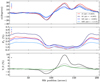 |
Fig. 1. Linear polarization angle (top panel) and total linear polarization fraction (middle panel) as a function of the position along the spectrograph’s slit at four different wavelengths in the wings of the Ca I line at 4227 Å. The various quantities are obtained by averaging the observed Stokes parameters over an interval of 50 mÅ, centered at the considered wavelength. These wavelengths are referred to as rI (red), bI (dark blue), bII (blue), and bIII (cyan), as discussed in the main text. The distance between the center of each interval and the center of the Ca I line (Δλ = λ − λ0) is indicated in the legend. For all figures the angle α is defined relative to a reference direction parallel to the nearest limb. In the bottom panel the amplitude of the blue peak of the V/I signal of Fe I 4224.2 Å (black line), Fe I 4228.7 Å (green line), and Ca I 4227 Å (gray line) are shown as a function of the slit position. The error bars are reported in the upper left of each panel. These data refer to a spectropolarimetric observation of a moderately active region close to the west limb performed on April 19, 2019. Figure adapted from Capozzi et al. (2020). |
We recall that the linear polarization angle is the angle between the direction of linear polarization and a reference direction, which in this work is taken parallel to the nearest limb. The linear polarization angle is defined within the interval between −90° and 90° (e.g., Landi Degl’Innocenti & Landolfi 2004), and is given by
with
This angle is positive when U/I > 0, meaning that the plane of linear polarization is rotated counter-clockwise relative to the above-mentioned reference direction. The total linear polarization fraction is given by
The bottom panel of Fig. 1 shows the variation with the slit position of the amplitude of the blue peak of the V/I signal of three different lines falling in the observed spectral interval, and forming in different atmospheric regions: Fe I 4228.7 Å (approximately mapping the middle photosphere, green curve), Fe I 4224.2 Å (approximately mapping the upper photosphere, black curve), and Ca I 4227 Å (region between upper photosphere and lower chromosphere, gray curve). Such spectral lines have effective Landé factors of  ,
,  , and
, and  , respectively. Information on the integration times for the above-mentioned observation, as well the uncertainties in the four Stokes parameters and in α and PL for each of the considered wavelengths, can be found in Capozzi et al. (2020). The corresponding error bars are reported in the top left corner of each panel in Fig. 1.
In Fig. 1 we highlight the appearance of three peaks, one negative and two positive, both in α (at the considered wing wavelengths) and in V/I. We recall that, for the relatively weak magnetic fields considered in this work, both these observables are sensitive to the longitudinal component of the magnetic field via the MO (see above) and Zeeman (Landi Degl’Innocenti & Landolfi 2004) effects, respectively. The comparison between the two positive peaks, found at the slit positions between 120″ and 140″ and between 155″ and 175″, reveals an interesting behavior. For all three considered lines, the V/I amplitude in the latter peak is substantially smaller than in the former, which is much more apparent for the lines forming in deeper layers (i.e., those corresponding to the black and green curves in the bottom panel). By contrast, the two peaks in α reach similar values, despite also being mainly sensitive to photospheric magnetic fields. The different behavior displayed by α and V/I indicates that these two observables are sensitive to different properties of the magnetic field. In PL, we observe that its sharpest variations occur when going from the quieter regions (characterized by small V/I and little variation in α) to those with a higher level of activity. This suggests that, compared to α, it is less sensitive to the magnetic field and more sensitive to other thermodynamic properties of the atmosphere, such as density and temperature.
3. Formulation and scope of the work
In the present article we investigate the diagnostic potential of α in the wings of the Ca I 4227 Å line to infer information on the longitudinal component of photospheric magnetic fields.
To this end, we numerically modeled the intensity and polarization profiles of this line by solving the RT problem for polarized radiation under non-local thermodynamic equilibrium (NLTE) conditions in a one-dimensional semi-empirical model of the solar atmosphere (see Alsina Ballester et al. 2017). Suitably modeling the broad wing linear polarization signals of this strong resonance line requires accounting for the frequency correlation between incoming and scattered radiation (or partial frequency redistribution, PRD; e.g., Faurobert-Scholl 1992). Its influence must be taken into account together with that of the magnetic field, through the Hanle, Zeeman, and MO effects. The numerical approach considered in this work is based on a rigorous quantum theory of polarization that can jointly account for all such effects (Bommier 1997).
Due to their strong influence on the broad wings of this line, our calculations also include the impact of a number of blended Fe I lines, which we modeled under the assumption of LTE, making use of the data presented in Kurucz (1993). We verified numerically that the influence of such blends is small or marginal at wavelengths close to bI, bII, bIII, or rI, which are the focus of the present work. Thus, the accuracy of the RT modeling of such blended lines is not critical for the reliability of our results (see Appendix A for more details).
4. Results
The synthetic profiles considered in this work are obtained from RT calculations, as described above, considering an LOS with μ = cos θ = 0.1, with θ the heliocentric angle, thus ensuring a large scattering polarization amplitude. For simplicity, we consider a magnetic field whose strength and orientation is constant at all heights in the atmospheric model. Recalling that the magnetic sensitivity in the wings is primarily due to the MO effects that are proportional to the longitudinal component of the magnetic field (Alsina Ballester et al. 2018), the calculations presented in this work consider horizontal magnetic fields contained in the plane defined by the vertical and the LOS.
4.1. Volume-filling magnetic field
In this section we consider the case of a magnetic field that occupies the entirety of the resolution element, which we hereafter refer to as volume-filling. The sensitivity of the scattering polarization wings of Ca I 4227 to such magnetic fields, calculated using the semi-empirical model C of Fontenla et al. (1993), hereafter FAL-C, is illustrated in Fig. 2. This figure shows that even relatively weak magnetic fields give rise to signals of considerable amplitude in the wings of the U/I profile and a conspicuous magnetic sensitivity in both the Q/I and U/I wings. Furthermore, as the magnetic field increases an overall decrease in the linear polarization fraction can also be clearly observed (for a more in-depth discussion, see Alsina Ballester et al. 2018). The magnetic sensitivity found in the line-core scattering polarization signal at similar field strengths is due to the Hanle effect. On the other hand, the circular polarization V/I signal found around the core region is produced by the Zeeman effect.
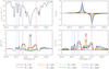 |
Fig. 2. Stokes I, V/I, Q/I, and U/I profiles of the Ca I 4227 Å obtained through the RT calculations described in the text. In this figure and those shown below, a LOS with μ = 0.1 is considered, and the magnetic fields are taken to be horizontal and contained in the plane defined by the vertical and the LOS. The FAL-C atmospheric model has been used for the calculations and field strengths between 0 G and 200 G are considered (see legend). The vertical lines indicate the wavelengths introduced in Capozzi et al. (2020), corresponding to rI (red), bI (dark blue), bII (blue), and bIII (cyan). A narrower spectral range is considered for the panel showing the Stokes V/I profile. The positive reference direction for Stokes Q is taken parallel to the nearest limb. |
The fact that the magnetic sensitivity of the various Stokes parameters at different wavelengths is driven mainly by different physical mechanisms is supported by compelling theoretical arguments (Landi Degl’Innocenti & Landolfi 2004; Sampoorna et al. 2009; Alsina Ballester et al. 2016). For the Ca I line considered here, we verified this through a numerical investigation based on response functions. The same investigation confirms that the magnetic sensitivity in the wing scattering polarization arises from MO effects, primarily due to the fields present in a narrow range of photospheric depths, extending roughly 300 km (see Appendix B for more details).
4.2. Magnetic fields occupying a fraction of the resolution element
In general, the magnetic field may permeate only a given fraction of the resolution element. The observed radiation results from the contribution from all spatial points within this area, each with its own magnetic field strength and orientation. It is well known that the circular polarization signals produced by the Zeeman effect are sensitive to the magnetic flux, but not to the fraction of the area that the magnetic field occupies. On the other hand, previous theoretical investigations (Alsina Ballester et al. 2019) hinted that the α value in the line wings may depend on this fraction and on the flux. In order to quantify this sensitivity, we assume that a uniform magnetic field is present in a fraction of the resolution element, whereas the rest is devoid of any magnetic field. We compare several realizations in which magnetic fields with different strength B are present within a different fraction f of the total area (or filling factor). These values were selected so that the average magnetic field over the resolution element, given by

which is proportional to the flux1, is the same for all cases. Specifically, we assumed f = 1 and B = 40 G (representative of a volume-filling magnetic field), f = 0.5 and B = 80 G, and f = 0.2 and B = 200 G, all corresponding to Bav = 40 G.
The observables α, PL, and V/I resulting from these realizations are shown in the top, middle, and bottom panel, respectively, of Fig. 3. The Stokes V/I signals found in the core of the Ca I line coincide for the three considered cases. We note that the RT code used in this investigation does not allow modeling the V/I signals in the nearby blended lines, and that the purpose of presenting such a comparison is only to emphasize that all the circular polarization signals produced by the Zeeman effect depend primarily on the magnetic flux when considering relatively weak magnetic fields as in the present work (e.g., Landi Degl’Innocenti & Landolfi 2004). By contrast, α and PL present clear differences between the three realizations, which can be found both in the line core, where they can be attributed to the impact of the Hanle effect, and in the line wings, where they are due to MO effects.
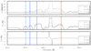 |
Fig. 3. Linear polarization angle α (top panel), linear polarization fraction PL (middle panel), and Stokes V/I (bottom panel) across the Ca I 4227 Å line, calculated in the FAL-C atmospheric model for an LOS with μ = 0.1. The various curves correspond to calculations considering horizontal fields with Bav = 40 G (see text), but different filling factors and field strengths: f = 1 and B = 40 G (dashed line), f = 0.5 and B = 80 G (dotted line), and f = 0.2 and B = 200 G (solid line). The vertical lines indicate the same wavelengths as in the previous figure. |
The magnetic sensitivity of the line wings is further highlighted by the results shown in Fig. 4, where the polarization angles at the bI (left panel) and bII (right panel) wing wavelengths are plotted as a function of Bav, considering horizontal magnetic fields with different filling factors. For each considered factor f (see legend) we took a series of realizations in which the field strength within the magnetized region B increases from 0 to 300 G in steps of 20 G, considering also the 10 G case. All such calculations were carried out considering both models C and P of Fontenla et al. (1993), representative of typical conditions of an average quiet region of the solar atmosphere and of a solar plage, respectively. For a given value of Bav, the polarization angle strongly depends on the value of f, sharply increasing with it. This is a finding of great diagnostic interest as it implies that the values of α at such wavelengths encode information on the fraction of resolution element occupied by the magnetic field, which can be directly obtained if an independent estimate of the magnetic flux is available. Such information may be accessible, for instance, from the circular polarization signals of photospheric spectral lines, and could be determined through the application of a number of widely known techniques, including for example the magnetograph formula or inversion codes that are freely available to the solar physics community (e.g., Ruiz Cobo & del Toro Iniesta 1992; Socas-Navarro et al. 2015).
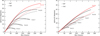 |
Fig. 4. Linear polarization angle α at the bI (left panel) and bII (right panel) wavelengths (see text) for an LOS with μ = 0.1 as a function of Bav considering horizontal magnetic fields with different filling factors f, for the atmospheric models FAL-C (solid line) and FAL-P (dashed line). For the sake of clarity, the curves corresponding to f = 1 are shown in red. |
We observe that this proposed diagnostic approach relies on the assumption that the strength and orientation of the magnetic field is constant with height in the solar atmosphere, similar to other commonly used diagnostic methods such as the magnetograph formula. In this case this assumption is justified on the grounds that the scattering polarization wings of the Ca I are sensitive, via MO effects, to the magnetic fields in a relatively narrow range of photospheric heights.
From Fig. 4 it can be seen that the sensitivity of α with respect to f is higher at the bI wavelength than at bII. This is a consequence of the larger impact of MO effects at wing wavelengths closer to the line center (see Appendix A). We also verified that this sensitivity is even lower at the bIII wavelength, while those at rI and bI are very similar to each other. The results of Fig. 4 also show that the magnetic sensitivity of α is appreciably model-dependent. Thus, in order to reliably use this observable to infer the magnetic filling factor, one must also obtain information about thermodynamic properties of the atmosphere, for instance, by making use of the above-mentioned inversion codes.
Furthermore, we find the polarization fraction PL (not shown in the previous figure) to be far less suitable as an observable for extracting information on the magnetic field. By contrast to α, which is zero in the absence of a magnetic field, its zero-field reference value is not known because it depends primarily on the radiation anisotropy in the solar atmosphere. For this reason, it is far more model-dependent than α, and therefore very precise information on the temperature and density stratification of the solar atmosphere would be necessary in order to reliably use it for magnetic diagnostics.
5. Conclusions
The present work builds upon the theoretical finding that the scattering polarization wings of strong resonance lines are sensitive to the longitudinal component of relatively weak magnetic fields through MO effects. For the Ca I 4227 Å line, this mechanism allows the investigation of photospheric magnetic fields in the gauss range, in which the Hanle effect also operates.
Further motivated by recent spectropolarimetric observations (Capozzi et al. 2020), the present investigation shows that the linear polarization angle α measured in the wings of the Ca I 4227 Å line encodes information not only on the magnetic flux, but also on the filling factor of the magnetic field, which remains hidden to diagnostic techniques based on the circular polarization signals produced by the Zeeman effect. This information can be directly obtained from α if the magnetic flux is known (e.g., by applying well-established Zeeman-based methods which rely on the weak-field assumption). Observations of this line with reasonably short integration times (see Capozzi et al. 2020) yield relatively low uncertainties for α in the wings, suggesting that such diagnostic methods should be suitable for applying valuable constraints on the filling factor of photospheric magnetic fields. Furthermore, observing that the core of the Ca I 4227 Å line forms in the lower chromosphere, the magnetic sensitivity of the scattering polarization in the wings (due to MO effects) can be exploited in combination with that in the core (due to the Hanle and Zeeman effects) to simultaneously obtain information on the magnetic fields present at different atmospheric heights, from the photosphere to the chromosphere.
The results of this work can also be applied to other strong resonance lines with extended wing scattering polarization signals. Notable examples are the H I Ly-α line at 1215 Å (Alsina Ballester et al. 2019), and the Mg II k line at 2795 Å (Alsina Ballester et al. 2016; del Pino Alemán et al. 2016, 2020), whose near wings originate at chromospheric heights. The magnetic sensitivity of α is necessarily model-dependent. The required information on the thermodynamic properties of the observed atmospheric region may be accessible through the application of state-of-the-art inversion codes. The findings shown in this article illustrate that new inversion codes fully accounting for the impact of magnetic fields of arbitrary strength and orientation in strong resonance lines, combining the Hanle, Zeeman, and MO effects, would be very valuable tools to access unexplored aspects of solar magnetism.
Acknowledgments
This research work was financed by the Swiss National Science Foundation (SNSF) through grants 200020_169418 and 200020_184952. E. A. B. and L. B. gratefully acknowledge financial support by SNSF through grant 200021_175997. L. B. and J. T. B. gratefully acknowledge financial support by SNSF through grant CRSII5_180238. J. T. B. acknowledges the funding received from the European Research Council through Advanced Grant Agreement no. 742265. IRSOL is supported by the Swiss Confederation (SEFRI), Canton Ticino, the city of Locarno and the local municipalities.
References
- Alsina Ballester, E., Belluzzi, L., & Trujillo Bueno, J. 2016, ApJ, 831, L15 [Google Scholar]
- Alsina Ballester, E., Belluzzi, L., & Trujillo Bueno, J. 2017, ApJ, 836, 6 [Google Scholar]
- Alsina Ballester, E., Belluzzi, L., & Trujillo Bueno, J. 2018, ApJ, 854, 150 [Google Scholar]
- Alsina Ballester, E., Belluzzi, L., & Trujillo Bueno, J. 2019, ApJ, 880, 85 [Google Scholar]
- Beckers, J. M., & Milkey, R. W. 1975, Sol. Phys., 43, 289 [Google Scholar]
- Bommier, V. 1997, A&A, 328, 706 [NASA ADS] [Google Scholar]
- Brückner, G. 1963, Z. Astrophys., 58, 73 [Google Scholar]
- Capozzi, E., Ballester, E. A., Belluzzi, L., et al. 2020, A&A, 641, A63 [NASA ADS] [CrossRef] [EDP Sciences] [Google Scholar]
- del Pino Alemán, T., Casini, R., & Manso Sainz, R. 2016, ApJ, 830, L24 [Google Scholar]
- del Pino Alemán, T., Trujillo Bueno, J., Casini, R., & Manso Sainz, R. 2020, ApJ, 891, 91 [CrossRef] [Google Scholar]
- Faurobert-Scholl, M. 1992, A&A, 258, 521 [NASA ADS] [Google Scholar]
- Fontenla, J. M., Avrett, E. H., & Loeser, R. 1993, ApJ, 406, 319 [Google Scholar]
- Gandorfer, A. 2002, The Second Solar Spectrum: A high spectral resolution polarimetric survey of scattering polarization at the solar limb in graphical representation. Volume II: 3910 Å to 4630 Å (vdf ETH) [Google Scholar]
- Kurucz, R. L. 1993, SYNTHE spectrum synthesis programs and line data [Google Scholar]
- Landi Degl’Innocenti, E., & Landi Degl’Innocenti, M. 1977, A&A, 56, 111 [NASA ADS] [Google Scholar]
- Landi Degl’Innocenti, E., & Landolfi, M. 2004, Polarization in Spectral Lines (Dordrechet: Kluwer) [Google Scholar]
- Ramelli, R., Balemi, S., Bianda, M., et al. 2010, in Ground-based and Airborne Instrumentation for Astronomy III, Proc. SPIE, 7735, 77351Y [NASA ADS] [Google Scholar]
- Ruiz Cobo, B., & del Toro Iniesta, J. C. 1992, ApJ, 398, 375 [Google Scholar]
- Sampoorna, M., Stenflo, J. O., Nagendra, K. N., et al. 2009, ApJ, 699, 1650 [Google Scholar]
- Socas-Navarro, H., de la Cruz Rodríguez, J., Asensio Ramos, A., Trujillo Bueno, J., & Ruiz Cobo, B. 2015, A&A, 577, A7 [NASA ADS] [CrossRef] [EDP Sciences] [Google Scholar]
- Stenflo, J. 2001, in Solar Magnetic Field: Zeeman and Hanle Effects, ed. P. Murdin, 2236 [Google Scholar]
- Stenflo, J. O., Baur, T. G., & Elmore, D. F. 1980, A&A, 84, 60 [NASA ADS] [Google Scholar]
- Stenflo, J. O., Solanki, S., Harvey, J. W., & Brault, J. W. 1984, A&A, 131, 333 [NASA ADS] [Google Scholar]
- Supriya, H. D., Smitha, H. N., Nagendra, K. N., et al. 2014, ApJ, 793, 42 [Google Scholar]
- Uitenbroek, H. 2006, in Solar MHD Theory and Observations: A High Spatial Resolution Perspective, eds. J. Leibacher, R. F. Stein, & H. Uitenbroek, ASP Conf. Ser., 354, 313 [NASA ADS] [Google Scholar]
Appendix A: Impact of the blends on the polarization angle
The calculations presented in this article include the impact of a number of blended Fe I lines (see Sect. 3). Given that these Fe I lines are relatively weak, and that their NLTE modeling would represent a major task, we modeled them under the assumption of LTE. Their impact was taken into account by adding at each point in the spectral grid of the RT calculations their opacity and emissivity contributions to those of the continuum. Here, we analyze the influence of these blends on the scattering polarization profiles through RT calculations like those presented in the main text of the article, considering the FAL-C atmospheric model, for an LOS with μ = 0.1. In this analysis we focus particularly on the reference wavelength positions introduced in the main text (bI, bII, bIII, and rI). The upper panel of Figure A.1 shows the Q/I profiles calculated in the absence of magnetic fields, comparing the results obtained when taking into account (solid curve) and neglecting the blends (dashed curve). For all the wavelengths of interest, highlighted with colored vertical lines (see legend), the blends appear to have a marginal impact, with the exception of rI. In the same panel, the magenta line indicates the wavelength position in the blue wing where the linear polarization amplitude is largest when all blends are neglected (hereafter bI′).
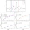 |
Fig. A.1. Results of RT calculations considering the FAL-C atmospheric model, for the radiation emerging at a LOS with μ = 0.1. The top panel shows the Q/I profile of the Ca I 4227 Å line as a function of wavelength, obtained in the absence of magnetic fields. The solid curve shows the profile obtained when including the effects of blends, and the dashed curve shows the profile obtained when neglecting them. The colored vertical lines give the wavelength positions of interest introduced in the article (see legend), with bI′ defined in the text. The bottom panels show the linear polarization angle α as a function of field strength, at the various wavelength positions of interest (see legend). These calculations were performed in the presence of a horizontal magnetic field contained in the plane defined by the local vertical and the LOS (see text). The solid and dashed curves represent the results obtained when accounting for the blends and neglecting them, respectively. |
The four lower panels show the variation of the linear polarization angle α with the magnetic field strength for the above-mentioned wavelengths, accounting for (solid curves) and neglecting (dashed curves) the impact of blends. As in the main text, the orientation of the magnetic fields is taken to be horizontal and contained in the plane defined by the LOS and the local vertical. The RT calculations were carried out for magnetic field strengths between 0 and 200 G in increments of 1 G. This figure clearly shows that the inclusion of blends has comparatively little impact on both the value of α and its magnetic dependence (compare the dashed and solid curves in the figure), even for rI. This supports the claim made in the main text that the accuracy in the modeling of the blends is not critical for the reliability of our RT calculations. In agreement with the results shown in Fig. 4, for all considered wavelengths, we find a monotonic increase of α with field strength, eventually reaching a plateau. We observe that such magnetic sensitivity depends on the considered wavelength, being stronger for those closer to the line core.
Appendix B: Response function
As pointed out in Sect. 4, depending on the considered spectral region, the magnetic sensitivity of the various Stokes parameters of the Ca I line is driven by different physical mechanisms. Here, this is illustrated through a numerical investigation based on response functions. The response functions (RFs, see Beckers & Milkey 1975; Landi Degl’Innocenti & Landi Degl’Innocenti 1977; Uitenbroek 2006) characterize the response of the intensity and polarization of the emergent radiation to the variation of a given physical quantity at any height and for a given wavelength. The RFs for the magnetic field for each of the Stokes parameters S = {I, Q, U, V} can be determined numerically through
where  , with
  and
and  the Stokes parameters at wavelength λ obtained when applying a perturbation up to height point z and without applying it, respectively. These Stokes parameters are obtained from RT calculations using atmospheric model FAL-C and for an LOS with μ = 0.1. We took the perturbation to be a 20 G horizontal magnetic field contained in the plane defined by the LOS and the local vertical, thus having ΔB = 20 G in Eq. (B.1). For
  this perturbation is applied form the lower boundary of the considered atmospheric model up to the spatial grid point corresponding to height z. In such calculations the impact of the blended lines was taken into account (see Sect. 3 and Appendix A for details).
To highlight the impact of Faraday rotation in the wing linear polarization signals, we computed the RFs both accounting for all MO effects in the spectral synthesis (see the upper four panels of Fig. B.1) and artificially setting to zero the anomalous dispersion coefficient ρV in the transfer equation (see the lower four panels of Fig. B.1). In order to ease this comparison, the RF for each Stokes parameter was normalized to its maximum absolute value for all heights and frequencies, considering both the calculations accounting for ρV and neglecting it2. It can be observed that the intensity and the linear polarization signals in the line core are most sensitive to variations in the magnetic field at depths corresponding to the middle chromosphere (between 800 and 1000 km). The magnetic sensitivity of the circular polarization signals, at the wavelength positions corresponding to their maxima, is strongest at slightly greater depths, centered at roughly 800 km. These results are in agreement with those of Supriya et al. (2014).
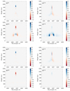 |
Fig. B.1. Response functions of the Ca I 4227 Å line, calculated in the FAL-C atmospheric model for an LOS with μ = 0.1. The upper four panels show, clockwise from the upper left, the RF for the Stokes parameters I, V, U, and Q, accounting for all MO effects. The bottom four panels show the RF for the same Stokes parameters, artificially setting the ρV coefficients to zero in the RT calculations from which the RF is computed. |
Farther into the line wings the magnetic sensitivity of the four Stokes parameters is strongest at considerably deeper layers of the solar atmosphere. The comparison between the RFs for Stokes Q and U obtained accounting for the above-mentioned MO effects and neglecting them indicates that the strong sensitivity in the wing linear polarization to magnetic fields at photospheric heights of around 300 km is almost entirely a consequence of such effects. In the wings the strongest response of the circular polarization is found at heights that correspond to a range that goes from the photosphere to the lower chromosphere. As wing wavelengths farther from the line core are considered, this sensitivity both weakens and is centered on slightly deeper regions.
All Figures
|
Fig. 1. Linear polarization angle (top panel) and total linear polarization fraction (middle panel) as a function of the position along the spectrograph’s slit at four different wavelengths in the wings of the Ca I line at 4227 Å. The various quantities are obtained by averaging the observed Stokes parameters over an interval of 50 mÅ, centered at the considered wavelength. These wavelengths are referred to as rI (red), bI (dark blue), bII (blue), and bIII (cyan), as discussed in the main text. The distance between the center of each interval and the center of the Ca I line (Δλ = λ − λ0) is indicated in the legend. For all figures the angle α is defined relative to a reference direction parallel to the nearest limb. In the bottom panel the amplitude of the blue peak of the V/I signal of Fe I 4224.2 Å (black line), Fe I 4228.7 Å (green line), and Ca I 4227 Å (gray line) are shown as a function of the slit position. The error bars are reported in the upper left of each panel. These data refer to a spectropolarimetric observation of a moderately active region close to the west limb performed on April 19, 2019. Figure adapted from Capozzi et al. (2020). |
| In the text | |
|
Fig. 2. Stokes I, V/I, Q/I, and U/I profiles of the Ca I 4227 Å obtained through the RT calculations described in the text. In this figure and those shown below, a LOS with μ = 0.1 is considered, and the magnetic fields are taken to be horizontal and contained in the plane defined by the vertical and the LOS. The FAL-C atmospheric model has been used for the calculations and field strengths between 0 G and 200 G are considered (see legend). The vertical lines indicate the wavelengths introduced in Capozzi et al. (2020), corresponding to rI (red), bI (dark blue), bII (blue), and bIII (cyan). A narrower spectral range is considered for the panel showing the Stokes V/I profile. The positive reference direction for Stokes Q is taken parallel to the nearest limb. |
| In the text | |
|
Fig. 3. Linear polarization angle α (top panel), linear polarization fraction PL (middle panel), and Stokes V/I (bottom panel) across the Ca I 4227 Å line, calculated in the FAL-C atmospheric model for an LOS with μ = 0.1. The various curves correspond to calculations considering horizontal fields with Bav = 40 G (see text), but different filling factors and field strengths: f = 1 and B = 40 G (dashed line), f = 0.5 and B = 80 G (dotted line), and f = 0.2 and B = 200 G (solid line). The vertical lines indicate the same wavelengths as in the previous figure. |
| In the text | |
|
Fig. 4. Linear polarization angle α at the bI (left panel) and bII (right panel) wavelengths (see text) for an LOS with μ = 0.1 as a function of Bav considering horizontal magnetic fields with different filling factors f, for the atmospheric models FAL-C (solid line) and FAL-P (dashed line). For the sake of clarity, the curves corresponding to f = 1 are shown in red. |
| In the text | |
|
Fig. A.1. Results of RT calculations considering the FAL-C atmospheric model, for the radiation emerging at a LOS with μ = 0.1. The top panel shows the Q/I profile of the Ca I 4227 Å line as a function of wavelength, obtained in the absence of magnetic fields. The solid curve shows the profile obtained when including the effects of blends, and the dashed curve shows the profile obtained when neglecting them. The colored vertical lines give the wavelength positions of interest introduced in the article (see legend), with bI′ defined in the text. The bottom panels show the linear polarization angle α as a function of field strength, at the various wavelength positions of interest (see legend). These calculations were performed in the presence of a horizontal magnetic field contained in the plane defined by the local vertical and the LOS (see text). The solid and dashed curves represent the results obtained when accounting for the blends and neglecting them, respectively. |
| In the text | |
|
Fig. B.1. Response functions of the Ca I 4227 Å line, calculated in the FAL-C atmospheric model for an LOS with μ = 0.1. The upper four panels show, clockwise from the upper left, the RF for the Stokes parameters I, V, U, and Q, accounting for all MO effects. The bottom four panels show the RF for the same Stokes parameters, artificially setting the ρV coefficients to zero in the RT calculations from which the RF is computed. |
| In the text | |
Current usage metrics show cumulative count of Article Views (full-text article views including HTML views, PDF and ePub downloads, according to the available data) and Abstracts Views on Vision4Press platform.
Data correspond to usage on the plateform after 2015. The current usage metrics is available 48-96 hours after online publication and is updated daily on week days.
Initial download of the metrics may take a while.