| Issue |
A&A
Volume 657, January 2022
|
|
|---|---|---|
| Article Number | A28 | |
| Number of page(s) | 18 | |
| Section | Stellar structure and evolution | |
| DOI | https://doi.org/10.1051/0004-6361/202039318 | |
| Published online | 24 December 2021 | |
First models of the s process in AGB stars of solar metallicity for the stellar evolutionary code ATON with a novel stable explicit numerical solver
1
Konkoly Observatory, Research Centre for Astronomy and Earth Sciences, Eötvös Loránd Research Network (ELKH), Konkoly Thege Miklós út 15-17, 1121 Budapest, Hungary
e-mail: This email address is being protected from spambots. You need JavaScript enabled to view it.
2
Instituto de Astrofísica de Canarias, C/Via Láctea s/n, 38205 La Laguna, Spain
3
Departamento de Astrofísica, Universidad de La Laguna (ULL), 38206 La Laguna, Spain
4
INAF-Osservatorio Astronomico di Roma, via Frascati 33, 00040 Monteporzio, Italy
5
School of Physics and Astronomy, Monash University, Clayton, VIC 3800, Australia
6
ELTE Eötvös Loránd University, Institute of Physics, Pázmány Péter sétány 1/A, Budapest 1117, Hungary
7
X Computational Physics (XCP) Division, Los Alamos National Laboratory, Los Alamos, NM 87545, USA
8
Computer, Computational and Statistical Sciences (CCS) Division, Los Alamos National Laboratory, Los Alamos, NM 87545, USA
Received:
1
September
2020
Accepted:
20
September
2021
Abstract
Aims. We describe the first s-process post-processing models for asymptotic giant branch (AGB) stars of masses 3, 4, and 5 M⊙ at solar metallicity (Z = 0.018) computed using the input from the stellar evolutionary code ATON.
Methods. The models are computed with the new code SNUPPAT (S-process NUcleosynthesis Post-Processing code for ATON), which includes an advective scheme for the convective overshoot that leads to the formation of the main neutron source, 13C. Each model is post-processed with three different values of the free overshoot parameter. Included in the code SNUPPAT is the novel Patankar-Euler-Deflhard explicit numerical solver, which we use to solve the nuclear network system of differential equations.
Results. The results are compared to those from other s-process nucleosynthesis codes (Monash, FRUITY, and NuGrid), as well as observations of s-process enhancement in AGB stars, planetary nebulae, and barium stars. This comparison shows that the relatively high abundance of 12C in the He-rich intershell in ATON results in an s-process abundance pattern that favours the second over the first s-process peak for all the masses explored. Also, our choice of an advective as opposed to a diffusive numerical scheme for the convective overshoot results in significant s-process nucleosynthesis for the 5 M⊙ models as well, which may be in contradiction with observations.
Key words: stars: abundances / stars: AGB and post-AGB / methods: numerical / nuclear reactions, nucleosynthesis, abundances
NuGrid collaboration, http://nugridstars.org
© ESO 2021
1. Introduction
Low- to intermediate-mass (initial mass in the range 0.8 M⊙ ≤ M ≤ 8 M⊙) thermally pulsing asymptotic giant branch (AGB; Iben & Renzini 1983) stars are predicted to contribute ∼50% of the cosmic abundances of elements heavier than iron in the Galaxy (e.g., Arlandini et al. 1999). These late-stage stars are structured as an inert CO core surrounded by a He-rich region (known as the He intershell) contained inside a H-rich convective envelope. Energy generation is alternately activated in two sites: the bottom of the He intershell through He burning and the H-burning shell through the CNO cycle. Depending on the active burning process, the star is found to be either in a thermal pulse (TP; He-burning phase) or an inter-pulse period (H-burning phase). There are two important changes in the stellar structure when the star goes through a TP (e.g., Herwig 2000). The first is the formation in the He intershell of a convective zone known as the pulse-driven convective zone (PDCZ). The second, which takes place after the PDCZ disappears, is the penetration of the H-rich convective envelope into the He intershell, a process known as the third dredge-up (TDU), which allows the products of He burning to reach the stellar surface.
Heavy element nucleosynthesis via the slow neutron-capture process (s process; e.g., Clayton et al. 1961) occurs in the He intershell of AGB stars (Schwarzschild & Härm 1967; Sanders 1967; Iben 1975b). The s process consists of a chain of neutron captures and β decays that increase the heavy nucleus abundances along the valley of stability. The s process takes place in the He intershell when enough free neutrons are present due to the activation of two neutron source reactions: 13C(α,n)16O and 22Ne(α,n)25Mg (see Sect. 2 for a more detailed description). During the TDU events, the products of the s process are mixed up to the stellar surface, where they can be observed, and they affect the chemical evolution of the Galaxy because they are ejected by the strong stellar winds that develop during the AGB (for a comprehensive review, see Karakas & Lattanzio 2014).
To understand both galactic and AGB chemical evolution, it is essential to study the s process with the help of numerical simulations that use information on AGB stellar structure evolution to calculate the s-process nucleosynthesis. Owing to the computationally expensive solution of the nucleosynthesis equations, a common approach (e.g., Karakas & Lugaro 2016; Pignatari et al. 2016) is to divide the calculation into two steps. The first step is to calculate the relatively computationally cheap stellar structure evolution with a nuclear network that contains only the most relevant reactions from an energetic point of view. The second step is to run a post-processing code using the stellar structure as an input and a more complete nuclear network capable of following the s-process nucleosynthesis. On top of temperatures and densities, information about the location and extent of the convective regions is needed to correctly simulate the PDCZ and the effect of TDU on the surface stellar abundances. A less common, but more realistic and computationally expensive, alternative is to solve the nucleosynthesis and structural equations simultaneously (e.g., Cristallo et al. 2015).
A traditional approach to solving a nuclear network is to use an implicit or semi-implicit numerical solver (Longland et al. 2014), that is, an integration method that uses information about future abundances to solve for those same future abundances. The advantage of such solvers is that they are numerically stable, keeping the future abundances bounded between a maximum and minimum value if the analytical solution is expected to be bounded as well (see e.g., Bader & Deuflhard 1983). The main disadvantage is that these solvers require the solution to an algebraic system of equations, which is computationally costly. In order to sidestep this disadvantage, we present the explicit Patankar-Euler-Deuflhard (PED) solver, which has the advantage of being numerically stable and does not require the solution to an algebraic system of equations.
Different AGB stellar evolutionary codes adopt different prescriptions to describe the physical processes inside AGB stars. Consequently, the predicted stellar structure evolution differs from code to code, affecting the nucleosynthesis calculations. In particular, the stellar structure evolutionary code ATON (Ventura et al. 1998, 2008) stands apart in that it uses the full spectrum of turbulence (FST; Canuto et al. 1996), a model for convection that takes the full spectrum of the eddies into account in the evaluation of the convective flux. Most stellar evolutionary codes instead use the mixing length theory (MLT; Böhm-Vitense 1958) scheme for convection, which only takes one large eddy into account. The use of the FST scheme along with other physical choices, such as the stellar wind prescription or the equation of state in the pressure ionisation regime, produces notable differences in several nucleosynthesis mechanisms. Examples of such mechanisms are the hot bottom burning (HBB) strength (that is, proton burning at the bottom of the convective envelope; see Mazzitelli et al. 1999), the number of TPs, and the maximum He intershell temperature. Analysing and comparing the s-process nucleosynthesis predictions obtained from the stellar structure provided by ATON to those calculated with other evolutionary codes can help us test the validity of the simulations of both the stellar evolutionary and nucleosynthesis processes. However, while there are s-process nucleosynthesis models for the codes that use the MLT convection scheme, no such calculations have been carried out for ATON, limiting its predictive capabilities (e.g., García-Hernández et al. 2013). With these calculations as our objective, we developed the SNUPPAT (S-process NUcleosynthesis Post-Processing code for ATON) code described in this paper.
The paper is structured as follows: A brief introduction to the s-process nucleosynthesis can be found in Sect. 2. The methodology of this work is split into Sect. 3.1, which presents the ATON models used as input for our post-processing code SNUPPAT, and Sect. 3.2, which describes the post-processing code itself, including the novel explicit numerical solver used in this work. The results are presented in Sect. 4, which deals with the formation of the main neutron source, 13C, in the post-processing code and presents the stellar surface abundances for a range of simulation parameters. Finally, the results are discussed and compared to other codes and observations in Sect. 5, and our final remarks and information on future work can be found in Sect. 6.
2. s-Process nucleosynthesis in AGB stars
As mentioned above, two neutron sources in the He intershell provide the free neutrons needed for the s process. The first is the 13C(α,n)16O reaction (e.g., Straniero et al. 1995; Gallino et al. 1998; Abia et al. 2001). This reaction takes place in a 13C-rich region known as the 13C pocket that forms when enough protons from the H-rich convective envelope are mixed into the 12C-rich He intershell during the deepest extent of the TDU through the 12C(p,γ)13N(β+,ν)13C reaction. This 13C burns radiatively during the inter-pulse period that lasts thousands to tens of thousands of years, generating a neutron density ∼108 cm−3. Its nucleosynthesis products are then engulfed into the PDCZ. Although the exact mechanisms of the proton mixing are unknown, several possibilities have been invoked, such as convective overshoot (e.g., Herwig et al. 1997; Herwig 2000; Cristallo et al. 2009), rotation (e.g., Herwig et al. 2003), gravity waves (Denissenkov & Tout 2003), and magnetic buoyancy (Trippella et al. 2016). This proton mixing must present a decreasing profile with a shallow enough slope (i.e. it must produce a partial mixing zone; see Goriely & Mowlavi 2000; Lugaro et al. 2003; Cristallo et al. 2009; Buntain et al. 2017) to result in a significant production of s-process elements. This is because where too many protons are mixed, 13C is destroyed, producing the neutron poison 14N through 13C(p,γ)14N, which captures the neutrons generated by the remaining 13C and inhibits the s-process nucleosynthesis. It is useful to define the quantity
 (1)
(1)
which, where greater than zero, is known as the effective 13C pocket (see Cristallo et al. 2009) and defines the region in which the s-process nucleosynthesis takes place for the 13C neutron source. Additionally, it has been predicted (Goriely & Siess 2004) that under a diffusive mixing approach, if the temperature at the bottom of the convective envelope where the 13C pocket forms is above ∼70 MK during the deepest extent of the TDU (known as a ‘hot TDU’), the 13C pocket is always contained inside a 14N pocket, inhibiting this neutron source altogether. These hot TDUs can be found to occur in initial masses above ∼4 M⊙ for solar metallicity and down to ∼3 M⊙ for lower metallicities.
The addition of a chemical mixing mechanism through rotation can also inhibit the 13C neutron source due to potential overlap of the 13C and 14N pockets. The main difference between this kind of inhibition and the one predicted in Goriely & Siess (2004), besides the intrinsic physical mechanism, is that chemical mixing through rotation can inhibit the 13C neutron source even in low-mass stars (Herwig et al. 2003; Siess et al. 2004; Piersanti et al. 2013), which contradicts the observational data of s-process enhanced objects such as Ba stars (Cseh et al. 2018). Moreover, recent simulations compared to asteroseismologic observations of the core rotation of giant stars indicate that rotation might not affect the s-process nucleosynthesis in a significant way (den Hartogh et al. 2019).
The second neutron source is the 22Ne(α,n)25Mg reaction (e.g., Cameron 1960; Iben 1975b,a; Busso et al. 1999; García-Hernández et al. 2006). This reaction occurs at the bottom of the PDCZ, which is rich in the 22Ne produced by two successive α captures on the 14N ingested from the H-burning ashes. This neutron source is limited by its high activation temperature of ≳300 MK, restricting it to the more massive (> 3 M⊙) of the intermediate-mass AGB stars (e.g., García-Hernández et al. 2006, 2009), and by the timescale of the PDCZ. Contrary to the 13C neutron source, the 22Ne neutron source acts in a much shorter timescale of decades, but provides a significantly higher neutron density of up to 1013 cm−3 (van Raai et al. 2012; Fishlock et al. 2014). Another key difference is that, because the 22Ne neutron source takes place at the bottom of the PDCZ, the enriched material is replenished by fresh material from the rest of the PDCZ, effectively further lowering the neutron exposure.
These two neutron sources produce markedly different s-process abundance patterns. In particular, at solar metallicity the 22Ne neutron source produces the elements of the first s-process peak (elements with a neutron magic number of 50, such as Sr, Y, or Zr, also known as the light s-process elements) and increases certain elemental ratios such as [Rb/Sr]1. The 13C neutron source produces elements of the second (magic number of neutrons of 82, such as Ba, La, or Ce, also known as the heavy s-process elements) and third (Pb) s-process peaks. There are two reasons for these unique signatures: (1) the different neutron densities, which activate different paths due to the possible activation of the s-process branching points, and (2) the time span during which each neutron source reaction is active, which changes the neutron exposure and, therefore, the relative production of the s-process peaks. We briefly review both mechanisms.
(1) Branching points are nuclei on the s-process path for which the fastest timescale can switch from the β-decay to the neutron capture reaction. A well known example of a branching point is 86Rb (e.g., van Raai et al. 2012), for which the probability of decaying before capturing a neutron increases from 2.58% for a neutron density of 108 cm−3 to 99.96% for a neutron density of 1013 cm−3. This branching point, along with that at 85Kr, leads to the creation of 87Rb, a long-lived (∼1010 years) Rb isotope with a magic number of 50 neutrons (e.g., García-Hernández et al. 2006). Because the neutron densities necessary to activate these branching points are restricted to the 22Ne neutron source, their activation signals the presence of this neutron source in AGB stars. Therefore, the abundance of Rb is an indicator of the neutron density attained in the stellar interior. A similar situation can be found for 135Cs (half-life of ∼106 years), which can only be produced from the stable 133Cs by neutron captures on the 134Cs (half-life of ∼2 years).
(2) The neutron exposure τ, defined as
 (2)
(2)
where Nn is the neutron density and uT is the thermal velocity, is the main predictor of the overall elemental s-process abundance distribution. Values below ∼0.4 mbarn−1 (calculated for a temperature of about 100 MK; see Fig. 2 of Herwig et al. 2003), heavily favour the first s-process peak over the second and third, while a higher neutron exposure increases the production of the second and third peaks instead. The reason is that due to the small neutron capture cross sections of isotopes with a magic number of neutrons, the s-process peaks act as bottlenecks on the s-process path, halting it until the abundance build-up of these isotopes brings the neutron capture probability on par with that of the nuclei before the peak. An increase in either the neutron density or the time that neutron-capture reactions are active increases the neutron exposure, enhancing the production of heavy elements with respect to lower neutron exposures.
3. Methods and models
As stated in the Introduction, our approach involves using the ATON stellar evolutionary code and a post-processing code that uses the ATON results as an input to accurately follow the s-process nucleosynthesis.
3.1. AGB modelling with FST
We used three models with initial masses of 3, 4, and 5 M⊙ and a metallicity of Z = 0.018 (scaled solar from Asplund et al. 2009) calculated with ATON. These models were run with 30 species from H to Si, those necessary to correctly follow the most important reactions for the stellar evolution, with the cross sections taken from the NACRE compilation (Angulo et al. 1999). For all the models we used the FST prescription for convection, with the fine tuning parameter β set to 0.2, consistent with previous works (e.g., Ventura et al. 1998; Mazzitelli et al. 1999). Regarding overshoot of the convective eddies into radiative stable regions, we assumed that convective velocities decay from the formal interface between the convective and radiative regions with an e-folding distance of ζHP, where ζ = 0.002; this choice is in agreement with the calibration based on the luminosity function of C-stars in the Large Magellanic Cloud given in Ventura et al. (2014). For the mass loss prescription, we used the Blöcker mass loss with a Reimers parameter of 0.02 (Blöcker 1995). Some of the stellar structure features are presented in Tables 1–3, respectively, for the 3, 4, and 5 M⊙ stars.
Physical characteristics related to the TDU events in a 3 M⊙ ATON simulation.
These models were chosen because each one represents a distinctly different regime from a nucleosynthesis perspective: The 3 M⊙ model surface composition is mostly changed due to TDU episodes and the presence of the 13C neutron source. The 5 M⊙ model surface composition is affected by a strong HBB and 22Ne neutron source activation. Lastly, the 4 M⊙ model sits in between, with a weaker HBB and 22Ne neutron source activation.
The TDU efficiency λ parameter2 and the ratio of dredged mass to envelope mass are the best indicators of the efficiency of envelope enrichment of each TDU event. The former is the measure of the proportion of the s-process enriched mass that is dredged to the surface, and the latter indicates the dilution of the s-process elements in the convective envelope. Higher values of any of these two quantities favour the stellar surface s-process enrichment, either by introducing more freshly synthesised material into the envelope, or reducing the dilution factor. The λ parameter found in the ATON models is generally lower than that found in other evolutionary codes, with the exception of FRUITY3. For example, Karakas (2014) finds λmax = 0.93 for a 4 M⊙ star at a metallicity of Z = 0.014, while Pignatari et al. (2016) have λmax ≈ 1.1 for the 4 M⊙ star at a metallicity of Z = 0.02, in contrast with the ATONλmax of 0.48 for the same initial mass.
Regarding the temperatures, ATON reaches higher temperatures both in the He intershell and at the base of the convective envelope (BCE) compared to other evolutionary models of the same core mass. These differences are determined by the use of the FST model for turbulent convection, which significantly affects the thermal stratification of the stellar regions laying close to the bottom of the outer convective envelope. These higher temperatures can affect both the 22Ne and 13C neutron sources. For the 22Ne neutron source, the higher temperature in the He intershell leads to a stronger activation than in other nucleosynthesis codes. In fact, this neutron source is active in the three masses presented here, with the 3 M⊙ star showing a marginal activation in those TPs where the maximum temperature reaches just above the 300 MK threshold.
For the 13C neutron source, the higher BCE temperature reached in ATON translates into an activation of the HBB at lower masses than other codes (see e.g., Sect. 7 of Ventura et al. 2018). In fact, the HBB already activates in ATON around an initial mass of 3.5 M⊙ (García-Hernández et al. 2013 and references therein), which means that the only carbon star (a star in which the surface C/O > 1) of the set presented here is the 3 M⊙ model. This is because the HBB activation burns C through proton captures, decreasing its surface abundance. Higher BCE temperatures also lead to more hot TDU events, which, as mentioned in Sect. 2, may inhibit the 13C neutron source.
3.2. SNUPPAT
3.2.1. Nuclear network solver
A post-processing code dedicated to the s process must correctly follow the nucleosynthesis equations for a large number (> 300) of species. Because nucleosynthesis processes are mathematically described by a coupled system of ordinary differential equations, and the reaction rates vary greatly between species (forming what is commonly known as a stiff system of equations), numerical instabilities arise during the integration unless specific care is taken in the choice of the integration method (see Longland et al. 2014). Common knowledge of numerical integration states that to avoid these numerical instabilities, an implicit or semi-implicit (linearised implicit) method is needed. The downside is that the number of operations necessary to advance each time step is greatly increased, which makes finding a fast and reliable method a priority. Our particular choice of numerical integration scheme is based on the Bader-Deuflhard (BD) method (Bader & Deuflhard 1983; Deuflhard 1983), a semi-implicit method with variable order of accuracy and automatic time step selection. The basic idea revolves around the use of a semi-implicit modification of the Gragg-Bulirsch-Stoer (GBS) algorithm (Gragg 1965; Bulirsch 1966). Here we were able to combine some of the techniques from the BD algorithm with a Patankar-type algorithm (e.g., Burchard et al. 2003, 2005) to obtain a completely original stable explicit solver for nucleosynthesis equations. We refer to this solver as the PED solver.
Before explaining the PED solver, we describe shortly the BD algorithm, because our solver is based on it.
The core of the BD algorithm solves the initial values problem,
 (3)
(3)
by dividing the integration step H into n sub-steps of size h = H/n with the following discretisation (Bader & Deuflhard 1983):
![Mathematical equation: $$ \begin{aligned}&\Delta _0 = (I - h J_{{ y}_0})^{-1} h(\eta _0)\nonumber \\&\Delta _k = \Delta _{k - 1} + 2(I - h J_{{ y}_0})^{-1} [hf(\eta _k) - \Delta _{k - 1}]\nonumber \\&\Delta _n = (I - h J_{{ y}_0})^{-1} [hf(\eta _n) - \Delta _{n - 1}]\nonumber \\&\eta (H, h) = \eta _n + \Delta _n, \end{aligned} $$](/articles/aa/full_html/2022/01/aa39318-20/aa39318-20-eq4.gif) (4)
(4)
where η0 = y0, ηk = ηk − 1 + Δk − 1, k = 1, …, n − 1, Jy0 is the initial Jacobian (df/dy) calculated for y = y0, and I is the identity matrix of the same size as the Jacobian. The array η(H, h) is the approximate solution of Eq. (3) after a time H for sub-steps of size h. Unfortunately, this algorithm requires the solution of the algebraic equation (I − hJy0)Y = X for different known X vectors. Although this can be made faster with the LU algorithm by decomposing once I − hJy0 per combination of y0 and h, it is still the slowest operation in the method.
The error expansion of this discretisation can be written as
 (5)
(5)
and allows for an efficient Richardson extrapolation such as that from the GBS algorithm. As an example, if the solution is re-calculated for a smaller sub-step of h′=h/2, one can see that
 (6)
(6)
with the drawback of having to perform twice the number of operations. One can then combine the solution with h and h′ to remove the g1(H) term, improving the convergence speed of the method. In Deuflhard (1983), the preferred extrapolation method is
 (7)
(7)
where Ti, 0 = η(H, hi) = η(H, H/ni). Once the Ti, k term has been calculated, the gk(H) term has been removed from the error expansion.
One can then calculate the kth relative error ϵk by using the Ti, k (see below for our particular choice) and test whether ϵk is below the desired tolerance, TOL. If the maximum ni is reached before that, then H must be reduced and the calculation tried again.
The next step is to choose the correct following H for the calculation. The basic formula for the error ϵk is
 (8)
(8)
Although, in principle, one can choose the last k, such that ϵk < TOL, Deuflhard (1983) takes into account the amount of work needed to arrive to that order, and whether it is better to aim for a smaller k, thus reducing the time step, or to attempt for an order increase (higher k and time step). The description of these steps is complex and outside of the scope of this paper, and if desired, they can be included in the same way for the BD algorithm and our solver.
The basic difference between our novel solver and the BD algorithm is the Patankar-Euler discretisation. In essence, this discretisation can be used for Eq. (3) if the right-hand side f(y) can be written as
 (9)
(9)
with K, D > 0, as is the case for nuclear networks. Then, Eq. (3) can be solved by using the following discretisation:
 (10)
(10)
where h is the time step chosen, Ki = K(yi), and Di = D(yi).
It is immediately apparent from Eq. (10) that this discretisation is unconditionally stable for any positive h. That is, that yi + 1 remains bounded even when h does not. However, the method itself does not require solving any algebraic equation, because all the terms on the right-hand side are known, making it much faster than the BD algorithm.
Unfortunately, the basic Patankar-Euler algorithm converges like the Euler method, that is, with a global truncation error proportional to h. We can accelerate the solver using a Richardson extrapolation, like for the BD algorithm. Unlike the BD algorithm, the Patankar-Euler error expansion does not contain only even powers of h. In fact, it can be shown to behave as
 (11)
(11)
It follows then that, for the Richardson extrapolation, we must use the recursive expression
 (12)
(12)
instead of Eq. (7).
The third and final difference between the BD algorithm and our novel solver, is that, instead of using Eq. (8) for the step size predictor, we must use
 (13)
(13)
With these three changes, we end up with a solver that combines the speed of the explicit methods with the stability of the implicit methods. The potential limitations of this solver lie on the stiffest of problems; however, our tests so far (Yagüe et al., in prep.) indicate that this solver behaves well for H burning, He burning, and both the main and the weak s process. A typical number of total sub-steps for the harder global integration steps during the s process may be of the order of 1000, divided among smaller integration steps of irregular size Hi each. We show the comparisons for both the main and weak s process between the backward Euler (BE), the BD algorithm, and this solver in Sect. 4.1.
Given that we have a powerful solver for the nucleosynthesis equations, and with the intention to easily parallelise the code, we chose to solve the changes to the abundance due to mixing and nucleosynthesis separately. We detail our specific numerical choices for each case below.
The use of an explicit method with automatic time step selection and accuracy monitoring makes it straightforward to follow all the coupled nucleosynthesis equations from neutrons to 210Po. For the results presented in this paper, we are using the 328 element nuclear network provided by Karakas & Lugaro (2016). Numerically, we allow a maximum average relative error of 5 × 10⁻⁵, this relative accuracy is calculated through the expression
 (14)
(14)
where  are the jth order Richardson extrapolations of the solution to species i for the kth index in the extrapolation sequence, yscale is a numerical lower limit to the abundances (10−24 in these calculations), N is the total number of species, and we use the extrapolation error as a proxy of the numerical approximation error. We note that we prefer not to use the initial abundances Yi for scaling the error to avoid some undesirable behaviours corresponding to rapid changes in the abundances. In particular, we want to prevent an artificial bottleneck to the calculation if it turns out that some
  is much larger than its corresponding initial abundance. In the same vein, we would like to avoid an underestimation of the error if the
  end up being much lower than the initial abundances. Tests done to the numerical methods used in SNUPPAT show that Eq. (14) is a good approximation of the error to the analytical solution for the required precision.
3.2.2. Mixing solver
We opted for a simplistic instantaneous mixing for the convective regions. However, for the overshoot mixing needed for the formation of the 13C pocket (see discussion in Sect. 2), we opted for a so-called linear, or advective, approach similar to that of Straniero et al. (2006), as opposed to the diffusive approach by Herwig et al. (1997) and Goriely & Siess (2004). We couple the mixing and nucleosynthesis mechanisms by using an operator-splitting approach, which consists in solving each process separately by solving the first process alone and using its solutions as initial values for the second process4. The differential equations we are using for overshoot mixing are
 (15)
(15)
where Yc is the instantaneously mixed abundance in the convective zone, Yj is the abundance in the radiative shell j, ξj is inverse of the time it takes for a mass element to travel from the convective zone to the shell j, and τj is related to ξj through abundance conservation. The coefficient ξj can be calculated as
 (16)
(16)
where rc and rj are the spatial coordinates of the edge of the convective region and the overshot shell, respectively, and uc is the turbulent velocity at the edge of the convective region. The relation between the overshoot velocity and uc, as well as the description for fthick, can be found in Ventura et al. (1998). As usual for these kinds of prescriptions, ω is the free overshoot parameter that is to be calibrated with observations. Values of ω larger than 0.14 are not explored due to numerical limitations. Specifically, values above ω ∼ 0.2 result in the introduction of protons into the PDCZ, where the instantaneous convection adopted here mixes them into the He-exhausted core, producing non-physical results.
The abundance profile resulting from solving the system (15) is a straight line in a logarithmic plot, with the ω parameter controlling the extent of the mixed region (known as partial mixing zone). A specific example for a 4 M⊙ model is depicted in Fig. 1, showing the difference between using ω = 0.10 and ω = 0.14.
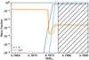 |
Fig. 1. Abundance profiles resulting from overshoot mixing using Eq. (15) with the parameters ω = 0.10 (dashed) and ω = 0.14 (solid) for a 4 M⊙ case. Not only does the extent of the overshot region grow with the increase in the free parameter, but the slope of the proton profile decreases, which results in wider effective 13C pockets. The convective envelope is shown as the hatched area. |
The fact that our overshoot method results in an exponential proton profile into the He intershell helps to compare it with other similar profiles, such as those detailed in Buntain et al. (2017). From that work and others, we know that we can expect an effective 13C pocket with a mass roughly half of that of the partial mixing zone. The main difference with the standard H inclusion profile of Buntain et al. (2017) is that we also find an extension of the convective envelope abundances into the He intershell. As an example, we note how in Fig. 1 the convective envelope abundances extend to the radiative region, and that this extension depends on the overshoot parameter. This additional completely mixed region is unavoidable for large enough overshoot parameters, given that when a deeper section of the He intershell is reached by the partial mixing, the earlier shells experience an increased mixing efficiency. This effectively represents an extension of the TDU with respect to the Tables 1–3 of around 10−4 M⊙. This behaviour is also reproduced in other simulations such as those computed with the FRUITY code, as can be seen in Fig. 5 of Cristallo et al. (2009).
To simulate the 22Ne neutron source, which burns convectively, we need to make sure that our operator-splitting along with instantaneous mixing approach is well suited to simulate this neutron source activation. In general terms, there are three possibilities regarding the interaction between convective mixing and the nuclear burning: (i) The nuclear burning is much faster than the convective mixing, (ii) the timescales for both processes are comparable, and (iii) the convective mixing is much faster than the nuclear burning. Among these three cases, only the last can be accurately simulated with an instantaneous mixing approach, while the first two require the solution of the convective mixing with a time-dependent algorithm.
In order to assess which of these regimes corresponds to the 22Ne(α,n)25Mg reaction within a PDCZ, we perform a comparison between the reaction and mixing timescales. The reaction timescale can be calculated by taking the typical PDCZ temperature in the ATON models between 4 and 6 M⊙, around 350 MK. At this temperature and with a 4He abundance of ∼0.2 mol g−1, we have a timescale for the 22Ne(α,n)25Mg reaction of
 (17)
(17)
Meanwhile, the mixing timescale can be approximated with the expression
 (18)
(18)
where u is the turbulent velocity and L the characteristic PDCZ length. By taking L to be ∼109 cm and u ∈ [104, 106] cm s−1, which are typical values for these PDCZ in ATON, we find that τdiff ∈ [103, 105], or that the mixing rate is between 10 and 1000 times faster than the burning rate. Therefore, the instantaneous convective mixing approach is a good enough simulation of reality when concerning this neutron source (e.g., Marigo et al. 2013).
We must point out, however, that our operator-splitting approach supposes that both the nuclear burning and the mixing have a time dependence that can approximate their behaviour to the real solution for arbitrarily small time steps. This supposition is critical for two reasons: (i) There are individual species, such as neutrons, for which the nuclear burning timescale is always orders of magnitude faster than any mixing process, and we cannot correctly model their behaviour if mixing instantaneously. We tested that the choice between mixing the neutrons along with the other species or burning them locally where they are created, appears to have no impact in the final s-process overabundances. This equivalence has been calculated and reported before in the literature (Hollowell & Iben 1990). (ii) The numerical approximation error cannot be assessed when one of the components acts instantaneously. This is because any way to measure this error depends on the possibility of obtaining the final results with an ever decreasing time step until the relative difference between two consecutive solutions are bounded by a tolerance imposed by the user, which is not possible to do if one of the processes is instantaneous. Given that our mixing implementation is not time-dependent, we briefly address its limitations.
First, we side-stepped the limitation on the calculation of the numerical approximation error by not making that calculation. Instead, we ensured a short enough time step by taking every one of the outputted ATON models in each post-processing simulation during a TP (when the time step between two models is approximately 0.1 years), and intercalating a number of instantaneous mixing episodes between the nuclear burning reaction calculations, such that no more than 0.02 years pass between mixing episodes. Second, we point out that the choice of an operator-splitting solution is unavoidable when taking an instantaneous mixing approach if we wish to avoid the one-shell burning approximation (that considers a constant T and ρ equal to an average on the mixing zone) to the convective regions. Conversely, operator-splitting allows for a very simple and effective parallelisation of the post-processing code.
The last situation where the mixing and burning happen at the same time is during the HBB. In this case, the mixing timescale at the BCE and the proton burning timescale are comparable (see e.g., Ritter et al. 2018) and can be in the timescale of years to days for ATON. The operator-splitting method is not accurate with an instantaneous mixing approximation when the burning and mixing timescales are similar (in particular for species such as Li). However, by reducing the timestep to approximately 0.01 years (around 100 hours), SNUPPAT can more closely follow the ATON HBB nucleosynthesis. Moreover, the final s-process abundance is not significantly affected (by less than a 4%) when the timestep is reduced to more closely simulate the HBB nucleosynthesis. This is expected due to the little effect that this timestep change has on He intershell 12C abundance (below 0.3%) and on the envelope hydrogen abundance (below 0.03%) in our models.
4. Results
4.1. Solver comparison
We implemented the PED solver in the NuPPN (NuGrid Post-Processing Network) code, where an implementation of the BD and BE methods already exist and are used for NuGrid nucleosynthesis calculations. This allows us to compare our solver directly to two already tested methods, showcasing its accuracy and speed. We decided to compare it in two trajectories: a He-burning trajectory in a 12 M⊙ star and a 13C pocket trajectory. For each method and trajectory, the basic time steps have been forcibly subdivided into a number of n = {1, 2, 4, 8, 16} steps, which the BD and PED solvers automatically divide further into sub-steps to calculate the Richardson expansion as described in Sect. 3.2.1. Each method was run with a tolerance of 10−3. This tolerance is the maximum error allowed according to the method error monitor. For example, for the PED solver this error is given by Eq. (14).
In Fig. 2 we show the error of each of the methods and chosen trajectories by choosing a single relevant isotope. The solutions are compared each to a calculation with the BD solver with n = 32 steps. Both the BD and PED solvers converge to the same L15 distance to the solution by n = 16 steps. It is likely that the BE converges also for larger values of n, owing to its lower convergence order.
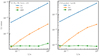 |
Fig. 2. L1 error (sum of the absolutes of the differences) for a chosen species and process when changing the number of steps n = {1, 2, 4, 8, 16} for each solver for the current NuPPN implementation. Each solution is compared to the solution yielded by the BD solver for n = 32 steps with a tolerance of 10−3. Left panel: final abundance for 16O in a 12 M⊙ He-burning trajectory. Right panel: final abundance for 138Ba for a 13C pocket trajectory. The BD and PED converge to the same solution. The slower convergence of the BE solver is due to its lower convergence order. |
In Fig. 3 we show the real time6 it takes for each solver to give a solution for a n number of steps. In the bottom panel the times are normalised to those of the BE solver. The main difference in times between the BD and the PED solvers, despite a similar accuracy of the solution, lies in solving the algebraic equation discussed before in the BD solver. Despite the PED solver requiring a higher number of iterations to achieve the same convergence order, the lower number of operations per iteration results in an overall much faster solution.
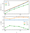 |
Fig. 3. Comparison of the time it takes for each solver to compute a solution for a 13C pocket trajectory. Top panel: time in absolute seconds. Lower panel: all the times normalised to the BE times. It is worth noting that even if BE is faster than BD, BE is less accurate for the same time steps, as shown in Fig. 2. The PED method is faster than the other two in all cases. |
4.2. Intershell 12C abundance
For consistency with the ATON models (Ventura et al. 2018; see also the ζ parameter in Sect. 3.1), we included overshoot at the bottom of the PDCZ with a value for the SNUPPAT overshoot parameter of ω = 0.002. This overshoot affects the s-process nucleosynthesis in several ways by increasing the 12C abundance in the He intershell, the TP luminosity and the maximum temperature, and the TDU penetration (Herwig 2000; Ventura et al. 2013). The effects of a higher intershell temperature and TDU penetration have been discussed in Sects. 2 and 3.1. Consequences of an increase in the 12C abundance in the He intershell for the 13C neutron source arise because the additional 12C is turned into additional 13C. A higher 13C abundance generates more free neutrons, which, therefore, increases the neutron exposure affecting the s-process abundance distribution (e.g., see Lugaro et al. 2003). The values of the ATON12C intershell mass fraction per pulse and initial mass are shown in Fig. 4. The difference in the He-intershell 12C abundance evolution between the 3 M⊙ and the other two models is explained by a more efficient TDU in the 3 M⊙ model, which drags more 12C to the surface than is replenished by the TP.
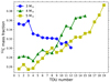 |
Fig. 4. Evolution of the He intershell 12C mass fraction during each of the TDU events represented in Tables 1–3. |
4.3. Formation of the 13C pocket
We ran three separate post-processing simulations for each mass with ω = 0.10, 0.12, and 0.14. The evolution and dependence of the effective 13C pocket mass extent and maximum 13C abundance on the ω overshoot parameter is shown in Fig. 5, and the average effective 13C pocket masses for each model are presented in Table 4. Although the absolute TP-averaged pocket mass depends on the ω parameter; the relative maximum  and the mass of each pocket for a given ω is controlled by the 12C mass fraction and the proton mixing profile. Because the overshoot mixing profile (Fig. 1) depends on ξj (that is, the inverse of the time it takes for a mass element to cover the distance from the convective envelope to the shell j) calculated by Eq. (16), we conclude that the relative differences between pockets for the same ω at different inter-pulse periods come from differences in either the pressure gradient or the turbulent velocity uc. In fact, the travelling time 1/ξj increases with a steeper pressure profile or a lower uc, resulting in a smaller overshoot mixing mass, and a less massive effective 13C pocket. Steeper pressure profiles as the star evolves can be a consequence, for example, of larger λ parameters.
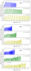 |
Fig. 5. Evolution of the effective 13C pocket in the 3, 4, and 5 M⊙ stars for the overshoot parameters ω = 0.10, 0.12, and 0.14. The y axis shows the mass fraction of effective 13C as defined in Eq. (1), while the x axis shows the width of the pockets in solar masses, with each pocket representing the widest mass extent of the effective 13C pocket in each inter-pulse. This occurs once the protons have burned completely in the He intershell but before the 13C starts to burn. The pockets are artificially arranged, with the earliest inter-pulse to the left to the latest on the right, to show the temporal evolution of their shape and size. There is not a one-to-one correspondence of the number of 13C pockets presented here and the number of TP shown in Fig. 4. This is because a higher ω forces a higher TDU efficiency, forming more 13C pockets. |
TP average of the effective 13C pocket mass extent  for each of the models presented here.
We point out that when running these post-processing simulations with different ω parameters, we are using the same ATON model calculated with a ζ = 0.002. This results in an inconsistency where the stellar structure does not react to the mixing of envelope material into the He intershell. This inconsistency is also found in other codes, such as Monash (e.g., Buntain et al. 2017), and its existence means that, in these codes, the s-process results must be understood with the caveat that there is no feedback between the overshoot (or partial-mixing zone, in the case of Monash) and the stellar structure. A more in-depth study on the feedback between overshoot extent and s-process nucleosynthesis due to changes in stellar structure in ATON is left to future work.
The average mass extent of the pocket decreases with the initial mass due to the shrinking of the He-intershell as the initial core mass increases and as the star evolves, and the increasing in absolute value of the pressure gradient (as already described by Cristallo et al. 2009, 2011, 2015).
Finally, the choice of overshooting scheme can have a profound effect on the formation of the 13C pocket. In particular, the inhibition of the effective 13C pocket during hot TDU events, as described by Goriely & Siess (2004), does not happen for our choice of overshooting scheme (given by Eq. (15)). The reason is that the overshot proton abundances are not connected with those of the neighbouring regions, only with the convective envelope. Therefore, the protons travelling from the envelope to the deeper layers cannot burn before reaching them, even if the temperature is high enough. Although the protons may quickly burn on arrival, the profile is not affected by these temperatures. To show this, we included a diffusive overshoot scheme in our code following Herwig et al. (1997) and performed two calculations during the same hot TDU in the 4 M⊙ model where the only difference between the calculations is the scheme used for overshoot. This test shows that for the same pulse the advective overshoot does not inhibit the effective 13C pocket (see Fig. A.1), while the diffusive one does (see Fig. A.2). We have included the figures for this test in Appendix A.
4.4. Stellar surface s-process results
The s-process nucleosynthesis results of our models are presented in Fig. 6 and Table 5. From Sect. 3.2 and Fig. 1 we know that the change in the overshoot parameter affects two important aspects of the nucleosynthesis calculation: the dredge-up efficiency parameter λ and the mass extent of the effective 13C pocket. An increase in either of these two quantities enhances the overall final stellar surface overabundance values. A larger dredged-up mass mixes more material from the intershell region into the convective envelope, naturally boosting the stellar surface overabundance values. A more massive 13C pocket results in s-process nucleosynthesis in a larger number of mass shells, which results in higher intershell overabundances and, therefore, higher stellar surface overabundances.
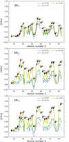 |
Fig. 6. Final stellar surface abundances of the elements heavier than Fe for the 3, 4, and 5 M⊙ ATON stars (top, middle, and bottom panel, respectively), post-processed with SNUPPAT with three different convective overshoot parameters, ω. The elements marked in red are those most sensitive to the neutron density. The breaks in the abundance distribution are due to the unstable isotopes Tc (Z = 43) and Pm (Z = 61). |
Selected final stellar surface overabundances.
Another critical aspect is the neutron exposure. This is tied to the 13C intershell mass fraction, which, in turn, depends on the 12C intershell mass fraction. Models with a higher 12C intershell abundance produce higher [hs/ls]7 ratios, that is, the relative production of the second to the first s-process peaks (Lugaro et al. 2003).
We start discussing the results with the 3 M⊙ star. As expected, the higher the ω parameter, the higher the stellar surface overabundances (see top panel of Fig. 6 and top rows of Table 5 for the 3 M⊙ model). The largest differences can be found around the s-process peaks. For example, the Ba abundance (represented by [Ba/Fe]), increases from approximately 0.7–0.9 dex when increasing ω from 0.10 to 0.14.
The abundance distribution (that is, the relative differences between the abundances of different elements) is for the most part independent of ω, with the only exception being the isotopes contributed by the 22Ne neutrons source, as can be seen from the [hs/ls] ratio that remains at ∼0.30 for almost every ω. The reason is that a larger ω only results in a more massive 13C pocket and greater TDU efficiency, not in a larger local neutron exposure. This independence of the abundance distribution for most isotopes with the mass extent of the partially mixed region is an intrinsic property of the models and is found also using the artificial partial mixing zone of Buntain et al. (2017). The [Rb/Sr] ratio in this 3 M⊙ model is negative, and decreases from −0.11 to −0.24 when increasing the ω parameter. This behaviour is consistent with the fact that the 22Ne neutron source is weakly activated and it is only mildly dependent on ω, as more massive effective 13C pockets increase the [Sr/Fe] without affecting [Rb/Fe].
In the 4 M⊙ star, the largest changes in abundances when changing ω are concentrated around the s-process peaks. However, the effect of the stronger activation of the 22Ne neutron source in this model, relative to the 3 M⊙ case, is clearly seen at both the first and second peaks in the increase in the [Rb/Sr] and [Cs/Ba] ratios. This is due to the activation of branching points, as discussed in Sect. 2. The [hs/ls] ratio is positive, but lower than the 3 M⊙ star. This is somewhat expected, given that the 22Ne neutron source favours the production of the first s-process peak at this metallicity. The increase in the [Rb/Zr] ratio from −0.01 to 0.11 and the [Cs/Ba] ratio before decay8 from −0.04 to 0.18 when incrementing ω from 0.10 to 0.14 (not shown in Table 5) is probably due to an increased amount of 14N, product of the more extended proton-mixed region in the He intershell. The additional 14N created by the larger overshoot is transmuted into 22Ne, which in turn boosts the efficiency of this neutron source.
The 5 M⊙ star behaves similarly to the 4 M⊙ case. An increase in the ω free parameter not only boosts the total stellar surface abundances, but also changes the elements Rb and Cs that are produced by branching points that depend on the activation of the 22Ne neutron source. Critically, the 13C neutron source is still active in this star, which may be in contradiction with the few observations of solar metallicity massive AGB stars at the beginning of the TP phase available in the literature, which show the lack of Tc suggesting the non-activation of the 13C neutron source (García-Hernández et al. 2013). This is a consequence of our numerical approach to the overshoot given that, as described in Sect. 4.3, a diffusive approach such as that of Goriely & Siess (2004) can prevent the formation of the effective 13C pocket.
5. Discussion
5.1. Comparison with the results from other codes
One of the most important uncertainties of the s-process nucleosynthesis simulations for low- and intermediate-mass stars is the formation of the 13C pocket. We described the formation of the 13C pocket in SNUPPAT in Sect. 4.3; here, we analyse the differences with the pocket formation in other simulations.
The  profiles of the Monash models (Buntain et al. 2017) have the most similar shape to those obtained in this work. Those are produced by an artificial proton profile within a partial-mixing zone of mass Mmix (a free parameter) at the deepest penetration of the convective envelope in the He-intershell during each TDU event. Taking the standard linear (in a log scale) hydrogen profile from that work, which covers log(XH) from 0 to −4 and forms an effective 13C pocket below around log(XH) = − 2, the mass extension of the effective 13C pocket is approximately half of the Mmix parameter. In the case of 3 and 4 M⊙, this means a 13C pocket mass extension between 5 × 10⁻⁴ and 10−3 M⊙ in their standard models. These effective 13C pockets are between two and five times larger than the largest average presented in Table 4.
We treat overshoot in a similar fashion as the FRUITY models. However, the proton profiles presented by Cristallo et al. (2009) for a 2 M⊙, Z = 0.014 case are ∼3 times larger in mass than those presented here for the 3 M⊙ case (our least massive case), when considering their β parameter (which is analogous to the parameter ω discussed in this work) in the range 0.075 to 0.125. This difference is likely related to the lower initial stellar mass of the FRUITY model we are comparing to, as the mass extent of the 13C pocket increases with decreasing initial mass. Another difference between the proton profiles in Figs. 1 and 2 of Cristallo et al. (2009) and in our Fig. 1 is that our H profile is approximately a straight line in logarithmic representation, while in FRUITY the slope of this H profile decreases in absolute value towards the inside of the star. We attribute this difference to the specific choice of the function of the velocity decay from the border of the convective zone. In the FRUITY models this depends on the distance from the BCE measured in Hp. In our models, it depends instead on the normalised pressure (see Eq. (16)). The effective 13C pocket mass extent of the FRUITY models with β = 0.1 is approximately 3 times larger than what we obtain with ω = 0.14.
Finally, we compare to the 13C pockets presented in Battino et al. (2016) and Pignatari et al. (2016) (that is, the NuGrid models), which come from diffusive overshoot9 as opposed the linear approach used by us and FRUITY. Despite this essential difference in the overshoot treatment, the proton profile obtained in Battino et al. (2016) is remarkably similar to what we obtain and, as a consequence, it produces an effective 13C pocket that resembles ours. In particular, from their Fig. 4 we recognise a similar shape and a mass extent of the same order of magnitude (∼10−4 M⊙) as those we obtain for an overshoot parameter of ω = 0.14. The effective 13C pockets presented by Pignatari et al. (2016) are much smaller than what we obtain. For example, in their Fig. 9, they present an effective 13C pocket of 5 × 10⁻⁶ M⊙ for a 5 M⊙ star, which is at least one order of magnitude lower than what we find for the same mass and metallicity. The difference between Battino et al. (2016) and Pignatari et al. (2016) is that in Battino et al. (2016) two diffusive steps are used. The consequence is a more extended partially mixed zone, resulting in a more massive effective 13C pocket and higher surface overabundances. For example, for a 2 M⊙ model at solar metallicity, Pignatari et al. (2016) produce pockets of ∼5 × 10⁻⁵ M⊙, almost an order of magnitude lower than those at 3 M⊙ while Battino et al. (2016) produce a ∼10−4 M⊙ effective 13C pocket for a 3 M⊙ simulation, which is only ∼2.5 times smaller than the average mass extension of the pockets we obtain. We do not include the models from Battino et al. (2019) in the interest of clarity, because for the relevant case (3 M⊙ and Z = 0.02) the overall production sits between that of Battino et al. (2016) and Pignatari et al. (2016) and so is covered by these two extremes.
5.2. Comparison of the s-process distributions
5.2.1. 3 M⊙ models
The 3 M⊙ comparison is presented in Fig. 7 and shows that the Monash model produces more s-process elements than the other codes. For example, the Monash [Ba/Fe] is ∼3 times higher than what we find for an overshoot parameter of ω = 0.14, while the [Sr/Fe] is 10 times higher than in our model. This can be explained by a combination of the λ parameter and the mass extent of the effective 13C pockets as discussed in Sect. 4.4. The Monash effective 13C pocket mass extent is around 10−3 for the model selected in Fig. 7, while in our models is ≲2.5 × 10⁻⁴ M⊙. The lower [hs/ls] fraction in Monash shown here is due to the lower effective 13C pocket mass fraction.
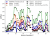 |
Fig. 7. Comparison of s-process nucleosynthesis results on the stellar surface of 3 M⊙ models at solar metallicity of Monash, FRUITY, NuGrid, and SNUPPAT. From Monash, we selected the Z = 0.14 model with Mmix equal to 2 × 10⁻³ M⊙ (Karakas 2014; Karakas & Lugaro 2016). From the FRUITY models, we selected the Z = 0.014 and Z = 0.02 models. From NuGrid, we chose the Z = 0.02 models from Battino et al. (2016), marked in the legend as ‘B16’, and Pignatari et al. (2016), marked in the legend with ‘P16’. |
Like with the Monash model, the FRUITY models show a more massive 13C pocket, but with a lower effective 13C mass fraction when compared to ours, and a similar λ parameter. This means that a lower neutron exposure is spread over a larger number of mass shells, resulting in an overall lower [hs/ls] ratio for a comparable or even larger overabundance than in the 3 M⊙ model with ω = 0.14 presented here.
For the NuGrid models, we included the results from applying the two different kinds of overshoot explained in Sect. 5.1. Battino et al. (2016) obtain a less massive effective 13C pocket, but a larger λ parameter, around two times larger than ours. The resulting stellar surface overabundances reported in Battino et al. (2016) are very similar to those produced by our ω = 0.14 model in both s-process peaks.
As can be seen in Fig. 7, the [hs/ls] ratio value covers a wide range in the results considered here. For example, both in the Monash models and the FRUITY models, this ratio is lower than 0.1 dex at solar metallicity (Z = 0.014 in FRUITY and Monash). On the other hand, the NuGrid models (Pignatari et al. 2016; Battino et al. 2016) find values closer to ours for 3 M⊙ models at solar metallicity (Z = 0.02), with ∼0.15 dex in Pignatari et al. (2016) and up to 0.25 dex in Battino et al. (2016) while, when using their definition for [hs/ls]10, our maximum sits at 0.14 dex.
These differences are explained by the intershell abundance of 12C, which affects the 13C mass fraction generated by proton captures, as outlined in Sect. 3.1. In the Monash models (Buntain et al. 2017), the intershell 12C mass fraction is below approximately 0.25, which means that the effective 13C mass fraction remains below 0.025, providing an [hs/ls] ratio of approximately zero. In the FRUITY models (see Cristallo et al. 2011, 2015), the 13C mass fraction is below 0.02, which results in a negative [hs/ls] ratio. Finally, the NuGrid models show an intershell 12C mass fraction between 0.4 and 0.5 (see Fig. 10 of Battino et al. 2016), resulting in a final [hs/ls] ratio similar to ours.
5.2.2. 4 M⊙ models
The nucleosynthesis of 4 M⊙ models is compared in Fig. 8. There are no models above 3 M⊙ in the work by Battino et al. (2016), so we compare to the Pignatari et al. (2016) results only. In the 4 M⊙ case, the 22Ne neutron source is strongly activated in all models except for FRUITY, where the effects of this neutron source cannot be seen in the surface s-process distribution. An explanation for this difference given by Karakas & Lugaro (2016) is that FRUITY models have fewer TDU episodes, and because the 22Ne neutron source generally activates more strongly towards the latest TPs, models with fewer TDUs will likely show fewer 22Ne neutron source effects in the surface. We find that this difference in number of TDUs exists in our case too, with the ATON 4 M⊙ model predicting 14 TDUs with λ > 0.05 and the 4 M⊙ FRUITY model at solar metallicity predicting only 8 TDUs above the same threshold.
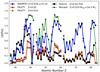 |
Fig. 8. Same as Fig. 7, but for 4 M⊙ models, except that we halve the value of Mmix for the Monash model. |
For this mass, although the standard Monash effective 13C pocket of 10−3 M⊙ is ∼4 times larger than that calculated by SNUPPAT with ω = 0.14 (both pockets having roughly half the mass extent of those found in the 3 M⊙ models), both codes predict abundances of approximately the same order. This is due to the fact that in SNUPPAT, the 22Ne neutron source activates more strongly than in Monash, providing higher neutron exposure for the nucleosynthesis. The stronger 22Ne neutron source activation is shown by the increase in the [Rb/Zr] ratio, higher in SNUPPAT than in Monash.
The FRUITY and NuGrid models both present much lower s-process overabundance than Monash and SNUPPAT. In the case of FRUITY, the 22Ne neutron source is not activated, which, along with the reduction with increasing initial mass of the 13C-pocket size, reduces the overall s production in FRUITY between the 3 M⊙ star and the 4 M⊙ star. This is further composed by the fact that FRUITY has smaller λ values than the other codes. In the NuGrid case, we infer from Pignatari et al. (2016) that a 4 M⊙ star should produce an effective 13C pocket with a mass extent between 5 × 10⁻⁵ and 10−6 M⊙. This is one to two orders of magnitude lower than what we obtain and is reflected in lower abundances than ours, particularly beyond the first s-process peak.
5.2.3. 5 M⊙ models
For the 5 M⊙ star (Fig. 9) the main difference relative to the comparisons for the 3 and 4 M⊙ models is that the standard Monash simulation has no partial mixing at the bottom of the convective envelope (i.e. no 13C pocket). This is motivated by the spectroscopic observations of solar metallicity massive AGB stars at the beginning of the TP phase (García-Hernández et al. 2013). Such stars display high Li coupled with low Rb and Zr and non-detection of Tc, which suggests the inhibition of the 13C neutron source. Given that our effective 13C is not inhibited by the hot TDU mechanism, we decided to add to the comparisons a 5 M⊙ model from Monash with a Mmix = 10−4 M⊙, which results in an effective 13C pocket of about 5 × 10⁻⁵ M⊙, roughly half the 1.10 × 10⁻⁴ M⊙ effective 13C pocket of the ω = 0.14 SNUPPAT case. For this reason, we decided to also include the ω = 0.12 calculation, which has an average mass extension of the effective 13C pocket of about 8.5 × 10⁻⁵ M⊙. This SNUPPAT model shows a better agreement with the Monash model. We note that the high Pb abundance in the ω = 0.14 model comes from the strong activation of both neutron sources, which does not happen in any of the other models presented here from FRUITY, Monash nor NuGrid.
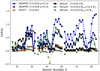 |
Fig. 9. Same as Fig. 7 but for 5 M⊙ models, except that we include Monash models with Mmix of 10−4 M⊙ and 0. We have also included a model with ω = 0.12 for SNUPPAT and removed one of the FRUITY models for clarity. |
Out of the models presented in Fig. 9, only those from non-standard Monash and SNUPPAT show an production factor in the second s-process peak of about 0.5 dex. The NuGrid model shows a greater first s-process peak resulting from a strong 22Ne neutron source activation. Both the FRUITY and standard Monash models (Mmix = 0 M⊙) show a small s-process overabundance, the consequence of an insignificant size of the effective 13C pocket.
5.3. Comparison to the observations
The products of the s-process nucleosynthesis in AGB stars can be measured in the AGB stars themselves (Abia et al. 2002; García-Hernández et al. 2006, 2007, 2013), the AGB binary companions enriched by AGB winds (e.g., Ba stars, Bidelman & Keenan 1951; de Castro et al. 2016), post-AGB stars (see van Winckel 2003 for a review, De Smedt et al. 2016), planetary nebulae (PNe; e.g., Schoenberner 1981; Sterling 2020), and stardust grains (e.g., Zinner 2014 for a review). Each source allows us to observe different evolutionary stages of the s-process nucleosynthesis, as well as different elements or even isotopes in the grains. The only site not included in this comparison is the post-AGB stars themselves because of the strong low-mass (< 3 M⊙), low-metallicity ([Fe/H] < −0.2) bias due to the short-lived nature of this evolutionary phase (e.g., van Winckel 2003; Reyniers et al. 2007; De Smedt et al. 2016). This lower mass and metallicity fall below those considered here.
We note that the comparisons in this section are limited for two main reasons: i) the first models presented here do not cover the full range of possible progenitor masses (especially the lower masses); and ii) there are several observational limitations; especially the low number of (key) elements that can be measured from stellar/nebular spectra and that strongly varies from C- and O-rich AGB stars to PNe and Ba stars.
At solar metallicity, only Rb and upper limits to Zr have been measured in massive O-rich AGB stars, while for C-rich AGB stars Rb, Sr, Y, and Zr are mostly available with additional Ba, La, Nd, Sm, and Ce abundances in only seven solar metallicity C-rich AGB stars. From PN nebular spectra Se, Br, Kr, Rb, and Xe are available in two PNe. Finally, for the Ba stars, only 5 s-process elements (Y, Zr, La, Ce, and Nd) are mostly available (with La being unreliable; Cseh et al. 2018 and sometimes Nb and Sm could be measured; e.g., Jorissen et al. 2019).
5.3.1. Carbon stars
We consider the carbon stars observed by Abia et al. (2001, 2002). These authors presented observations of a number of s elements such as Rb, Sr or Ba as well as Tc in carbon-rich AGB stars. The key measurement of radioactive Tc was made to discriminate between intrinsic s-process-enhanced stars (where the s-process enhancement is produced in the star, henceforth ‘intrinsic s star’) and extrinsic s-process-enhanced stars (s-process enhancement obtained after a mass transfer from a companion AGB star, henceforth ‘extrinsic s star’), where the presence of Tc indicates the former and its absence the latter. We compare our models to the Ba abundance from this work to calibrate our ω parameter (we included the abundances we are comparing to in Table B.1). The median [Ba/Fe]11 abundance of the intrinsic s stars observed by Abia et al. (2002) is 0.75 with an uncertainty of 0.30, leaving the three choices for our ω parameter well within this observational constraint for the 3 M⊙, which is the only among our models that becomes a C star. In Fig. 10 we show the [hs/ls] ratio versus the [s/Fe] ratio12 as they evolve with time in our 3 M⊙ models along with the data by Abia et al. (2001, 2002). We can see that our results for five out of the seven objects fall within the observational uncertainties, with the other two likely being lower-mass stars.
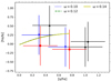 |
Fig. 10. Observed [s/Fe] and [hs/ls] ratios for solar metallicity C stars from Abia et al. (2001, 2002) alongside the evolution of ratios for the 3 M⊙ models. The red squares are stars with ‘doubtful’ Tc detection. The blue inverted triangles are stars with bolometric magnitude lower than −5.5, which should correspond to the more massive among the sample, closer to our 3 M⊙ simulations. The black triangles are stars with bolometric magnitude higher than −5.5 and Tc detection. The uncertainties are those given in Abia et al. (2001, 2002). |
A more comprehensive way to select the best overshooting parameter may be a comparison with the individual elemental abundances (between 7–9 elements, depending on the star) reported by Abia et al. (2001, 2002). Because for AGB stars we are not necessarily witnessing the final composition (see Fig. 10), we compared, for each star, all the model predictions from the 3 M⊙ simulation with the abundances observed. In order to find the best fit, we calculated the average L2 error (i.e. the squared difference) between the surface abundances in the simulation and the observed surface abundances. The values for the best fit for each one of the 3 M⊙ runs are shown in Table 6. Interestingly, this table shows that the best fits are obtained for (i) the more luminous stars (Mbol ≤ −5.7) with Tc (in principle, the higher-mass intrinsic AGB stars in the sample) or (ii) the stars with doubtful Tc, which might be extrinsic s stars. Overall, the overshoot parameter of ω = 0.14 gives the best fit for all the observations.
Comparison with carbon star observations.
5.3.2. Planetary nebulae
In Fig. 11 we show the abundances from Madonna (2018) (and references therein, such as García-Rojas et al. 2015; Madonna et al. 2018) observed in PNe NGC 3918 and NGC 7027 along with our final selected surface abundance results presented in Fig. 6 for the 3 and 4 M⊙ stars. We selected these two PNe because they have the most complete and recent solar metallicity PNe observations in regards to neutron-capture elements. As can be seen in the figure, the PNe measurements show an opposite trend for the [Kr/Rb] ratio than our s-process models in the range of masses considered here. This ratio may be reversed for less massive stellar models, as is the case with Monash models from 1 to 3 M⊙ (Madonna 2018). Finally, we point out that one important conclusion of Madonna (2018) is that PNe that show evidence of HBB activation have low s-process production (see the case of NGC 2440). This observation hints towards either the activation of the hot TDU mechanism that inhibits the 13C source in more massive stars, in contrast with our models, or the shortening of the AGB lifetime due to a mass transfer scenario.
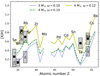 |
Fig. 11. Observed abundances from Madonna (2018) of PN NGC 3918 (open triangles) and NGC 7027 (filled squares) alongside the best fitting of our overabundance results (lines and filled dots). In grey are shown the uncertainties for each of the measurements. |
5.3.3. Barium stars
In addition to the previous calibration, we can place our results in context with the work on Ba stars presented by de Castro et al. (2016) and Cseh et al. (2018). These stars are extrinsic s stars, which means that the observed abundances are diluted with respect to those of the intrinsic s stars. The effects of this dilution are not trivial when transforming from the intrinsic s-star abundances to the extrinsic s-star abundances. For example, if we consider that a fraction k of the extrinsic s-star envelope mass has been added and mixed from the intrinsic s-star envelope, the abundances are related by
![Mathematical equation: $$ \begin{aligned} \left[X/\mathrm{Fe}\right]_{\rm e} = \log _{10}\left(\left(1 - k\right) + k10^{\left[X/\mathrm{Fe}\right]_{\rm i}}\right) , \end{aligned} $$](/articles/aa/full_html/2022/01/aa39318-20/aa39318-20-eq26.gif) (19)
(19)
where the sub-indices i and e represent the abundances from the intrinsic s star and extrinsic s star, respectively, and considering that the AGB envelope iron abundance is not significantly modified. This means that, in general, the quantities in Table 7 are affected by the dilution process. However, we can safely assert that, for the values presented in Table 7 (that correspond to a k = 1), [Y/Fe] and [Ce/Fe] are more affected than the [Ce/Y] ratio when k < 1. This is because the dilution process will affect both Ce and Y while leaving Fe unchanged, due to both AGB and the companion star having the same Fe abundance.
Average of [Y/Fe] and [Ce/Fe] as well as ratio [Ce/Y] by mass and overshoot parameter, ω, from our simulations.
We can compare our results of Table 7 to Fig. 6 of Cseh et al. (2018), where the bulk of [Ce/Y] values at solar metallicity range from −0.4 dex to below 0.2 dex. At this metallicity, our [Ce/Y] ratios are above the trend shown by the observations, slightly above the 4 M⊙ FRUITY and Monash ratios. If we consider dilution in the range of 0.1 < k < 0.5, our results move towards the bulk of the measurements, although remaining with the positive [Ce/Y] abundances. Because the masses of both the observed and the companion stars are estimated to be in the range of 1 to 4 M⊙, we included our 3 and 4 M⊙ models in the comparison.
Similarly to the C-rich AGB stars, we compared the individual abundances observed in the solar metallicity Ba star BD-142678 (de Castro et al. 2016) with those predicted by our best fit 3 and 4 M⊙ models with ω = 0.14. We selected this particular Ba star because its progenitor mass is inferred to be 3 M⊙ (i.e. closer to our models), when compared with both Monash and FRUITY model predictions diluted to fit the observed [Ce/Fe] ratio (Cseh et al. 2020). The comparison is shown in Table 8, where we also list the dilution factor k needed to get the best match as well as the average L2 errors. It should be noted that for the 3 M⊙ star model we report a value of k = 1, which corresponds to the maximum possible value for k, not necessarily the value with the best fit, which needs k > 1. Such a value would require yields that are not attainable by diluting our model. If we try to fit the observed [Ce/Fe] ratio, then our best fit 3 M⊙ model would need a dilution of k = 0.83, which is very close to the dilution value of 0.93 for the 3 M⊙ FRUITY model fitted for this Ba star by Cseh et al. (2020).
Comparison with Ba star individual observed abundances.
5.3.4. Massive AGB stars
Another test of our simulations is a comparison with the observed [Rb/Fe] abundances in massive solar metallicity AGB stars. Some of the first observations of the [Rb/Fe] ratio (with a typical large uncertainty up to ±0.8 dex) were obtained by García-Hernández et al. (2006), who reported values ranging from −1.0 to 2.5 dex. More recent work by Zamora et al. (2014) and Pérez-Mesa et al. (2017) narrows this spread to values between −0.7 and 1.3 dex with an uncertainty of ±0.7 dex. As can be seen from Fig. 6, our [Rb/Fe] values fall well within those constrains for our more massive models. However, the [Rb/Zr] ratios reported in Zamora et al. (2014) and Pérez-Mesa et al. (2017) range from −0.3 dex to 0.7 dex with uncertainties between 0.7 and 1 dex, while in our 4 and 5 M⊙ models we find that the [Rb/Zr] ratio remains between −0.1 and 0.1 dex. This is consistent with the ratios found by other groups. This gap between models and observation has been discussed in the literature before, and may be attributed to the different dust condensation temperatures of Zr and Rb, with Zr being removed from the gas at higher temperatures than Rb (see e.g., García-Hernández et al. 2009; van Raai et al. 2012).
5.3.5. Dust grains
Finally, we compare to isotopic ratios of s-process elements measured in meteoritic silicon carbide (SiC) (Lugaro et al. 2018). Most of these grains formed in AGB C-rich stars such as our 3 M⊙ model (see Dell’Agli et al. 2015 and references therein) and carry information on the s-process nucleosynthesis of the stars where they formed (e.g., see Liu et al. 2014; Lugaro et al. 2014). Certain isotopes, such as those of Zr, strongly depend on the s-process neutron density due to a branching point in 95Zr, as well as both the neutron exposure and s-process production given by the effective 13C pocket mass fraction and mass extension. By comparing our results (Table 9) with Fig. 2 of Lugaro et al. (2018), we find that our 3 M⊙ models cover some of the observed values of δ91Zr/94Zr13, δ92Zr/94Zr, and δ96Zr/94Zr, with larger ω values agreeing better with the observed ratios. In fact, our 3 M⊙ models are very similar to the ‘M2.z2m2’ points shown in Fig. 14 of Battino et al. (2016), just shifted left towards the bulk of the measurements. This is expected because our high [hs/ls] for this 3 M⊙ model is produced by a high neutron exposure due to the large effective 13C mass fraction, which is also tied to a high neutron density for the 13C neutron source and the partial activation of the 22Ne neutron source due to the higher temperature.
Comparison with Zr dust grains.
6. Conclusions
We have presented new s-process nucleosynthesis predictions based on the ATON stellar evolutionary models at solar metallicity (Z = 0.018) for stars of 3, 4, and 5 M⊙. These results show that:
-
In the more massive AGB stars (≳4 M⊙), our overshoot prescription does not find the effective 13C pocket inhibition described by Goriely & Siess (2004). This is because the overshoot scheme adopted in SNUPPAT is advective instead of diffusive. Therefore, for simulations where hot TDU episodes are expected to inhibit the effective 13C pocket, this overshoot prescription should not be used. If a diffusive overshoot scheme is implemented instead, the 13C pocket may be inhibited in our 4 and 5 M⊙ cases because in ATON both those stars experience hot TDU episodes for most of their lifetimes. This may also be the reason for the slight disagreement with the PN observations, in particular the lower s-process yield of some of them. This needs to be investigated in future work.
-
The envelope overshoot parameter of ω = 0.14 reproduces the observed abundance of [Ba/Fe] well for solar metallicity carbon stars. This parameter also yields the best agreement with other standard s-process nucleosynthesis models, especially for the first and second s-process peaks. We note that this overshoot parameter is a consequence of post-processing models that have inconsistent overshoot with the structure models. If the overshoot feedback were included in the structure models, it is likely that we would obtain a smaller overshoot parameter.
-
Due to the high 12C intershell mass fraction, our models produce a higher neutron exposure and [hs/ls] value than the Monash and FRUITY models of the same mass. For stars of < 4 M⊙, we find very similar results to NuGrid despite our different approaches to the overshoot mechanism.
-
The ATON models achieve a high intershell maximum temperature, efficiently activating the 22Ne neutron source for the 4 and 5 M⊙ models and producing high [Rb/Fe] ratios, in accordance with observations of massive AGB stars. Although the [Rb/Zr] ratios are much lower than those observed, they remain in agreement with the other s-process nucleosynthesis models.
-
Some of the isotopic Zr dust grain measurements can be reproduced by our C-rich 3 M⊙ model, although there is still some disagreement with the δ96Zr/94Zr value for the bulk of the measurements, which is likely attributable to the high neutron exposure occurring in our simulations. The ω necessary to reproduce these results could be lower if the feedback between overshoot and structure were taken into account.
We have also introduced a new explicit integration method, the PED solver, and we have shown that an implementation in NuPPN is as accurate as the BD solver and faster than both the BD and BE implementations for the same tolerance in He burning and 13C pocket trajectories.
The natural extension of this work is to explore s-process abundances produced by ATON models for sub-solar and super-solar metallicities and to extend our mass range to lower and higher initial stellar masses. Furthermore, we will experiment with different overshoot and convective mixing prescriptions to understand the effects that both hot TDU episodes and the HBB can have on the s-process overabundances depending on the numerical modelling. Finally, we will also explore more systematically the effects of the feedback between overshoot and stellar structure on s-process nucleosynthesis.
The bracket notation [A/B] is defined as log(YA/YB) − log(YA/YB)⊙, where YA is the number fraction of element A.
λ = ΔMdredge/ΔMcore, where ΔMdredge is the TDU penetration into the He intershell and ΔMcore is the growth of the H-exhausted core during the previous inter-pulse.
As an example, we can consider the linear equation y′=(a − b)y with solution y = y0exp[(a − b)Δt]. We obtain the same expression by solving first the equation, y′=ay, for Δt and then taking the solution y = y0exp(aΔt) as the initial value for the equation y′= − by and solving it for Δt as well. Although the operator-splitting method is only exact for linear equations, it remains a useful technique for non-linear equations too.
Defined as the sum of the absolutes of the differences.
That is, the time in seconds that the program takes to run according to a real clock.
Where [hs/ls] is defined as the difference between [hs/Fe] and [ls/Fe]. The ratio [ls/Fe] is the average of [Sr/Fe], [Y/Fe], and [Zr/Fe], and the ratio [hs/Fe] is the average of [Ba/Fe], [La/Fe], and [Ce/Fe]; see e.g., Karakas & Lattanzio (2014).
The values presented in the tables and figures of this paper are decayed for 104 years to remove some of the transient features displayed by short-lived isotopes, such as those from 135Cs.
In the NuGrid papers, the term ‘convective boundary mixing’ is used instead of overshoot. However, for consistency with the nomenclature of this work, we use the term overshoot to refer to this boundary mixing as well.
The definition of [hs/Fe] used in Pignatari et al. (2016) is slightly different to what we use as they chose the average of [Ba/Fe], [La/Fe], [Nd/Fe], and [Sm/Fe].
Although the value is given in [Ba/M], with the metallicity, M, being an average of Ca, Ti, V, Fe, and Co, we decided to leave the ratio with respect to Fe for consistency. Both values are virtually identical, with a typical [M/Fe] ∼ −0.002 dex.
The [s/Fe] ratio is calculated as the average of all the [X/Fe] ratios used for the [hs/Fe] and [ls/Fe] calculations.
The δ notation is the per mil variation compared to the solar ratios, which are δ = 0 by definition.
Acknowledgments
This work has been supported by the European Research Council (ERC-2016-CO Grant 724560) and by the US Department of Energy LDRD program through the Los Alamos National Laboratory. Los Alamos National Laboratory is operated by Triad National Security, LLC, for the National Nuclear Security Administration of US Department of Energy (Contract No. 89233218NCA000001). D.A.G.H. acknowledges support from the State Research Agency (AEI) of the Spanish Ministry of Science, Innovation and Universities (MCIU) and the European Regional Development Fund (FEDER) under grant AYA-2017-88254-P. C. D. acknowledges support from the Lendület-2014 Programme of the Hungarian Academy of Sciences. We thank the anonymous referee for their useful comments that improved the quality of this work.
References
- Abia, C., Busso, M., Gallino, R., et al. 2001, ApJ, 559, 1117 [Google Scholar]
- Abia, C., Domínguez, I., Gallino, R., et al. 2002, ApJ, 579, 817 [NASA ADS] [CrossRef] [Google Scholar]
- Angulo, C., Arnould, M., Rayet, M., et al. 1999, Nucl. Phys. A, 656, 3 [Google Scholar]
- Arlandini, C., Käppeler, F., Wisshak, K., et al. 1999, ApJ, 525, 886 [Google Scholar]
- Asplund, M., Grevesse, N., Sauval, A. J., & Scott, P. 2009, ARA&A, 47, 481 [NASA ADS] [CrossRef] [Google Scholar]
- Bader, G., & Deuflhard, P. 1983, Numer. Math., 41, 373 [CrossRef] [Google Scholar]
- Battino, U., Pignatari, M., Ritter, C., et al. 2016, ApJ, 827, 30 [NASA ADS] [CrossRef] [Google Scholar]
- Battino, U., Tattersall, A., Lederer-Woods, C., et al. 2019, MNRAS, 489, 1082 [Google Scholar]
- Bidelman, W. P., & Keenan, P. C. 1951, ApJ, 114, 473 [Google Scholar]
- Blöcker, T. 1995, A&A, 297, 727 [NASA ADS] [Google Scholar]
- Böhm-Vitense, E. 1958, Z. Astrophys., 46, 108 [Google Scholar]
- Bulirsch, R., & Stoer, J. 1966, Numer. Math., 8, 1 [CrossRef] [Google Scholar]
- Buntain, J. F., Doherty, C. L., Lugaro, M., et al. 2017, MNRAS, 471, 824 [NASA ADS] [CrossRef] [Google Scholar]
- Burchard, H., Deleersnijder, E., & Meister, A. 2003, Appl. Numer. Math., 47, 1 [Google Scholar]
- Burchard, H., Deleersnijder, E., & Meister, A. 2005, Ocean Dyn., 55, 326 [NASA ADS] [CrossRef] [Google Scholar]
- Busso, M., Gallino, R., & Wasserburg, G. J. 1999, ARA&A, 37, 239 [Google Scholar]
- Cameron, A. G. W. 1960, AJ, 65, 485 [CrossRef] [Google Scholar]
- Canuto, V. M., Goldman, I., & Mazzitelli, I. 1996, ApJ, 473, 550 [NASA ADS] [CrossRef] [Google Scholar]
- Clayton, D. D., Fowler, W. A., Hull, T. E., & Zimmerman, B. A. 1961, Ann. Phys., 12, 331 [NASA ADS] [CrossRef] [Google Scholar]
- Cristallo, S., Straniero, O., Gallino, R., et al. 2009, ApJ, 696, 797 [NASA ADS] [CrossRef] [Google Scholar]
- Cristallo, S., Piersanti, L., Straniero, O., et al. 2011, ApJS, 197, 17 [NASA ADS] [CrossRef] [Google Scholar]
- Cristallo, S., Straniero, O., Piersanti, L., & Gobrecht, D. 2015, ApJS, 219, 40 [Google Scholar]
- Cseh, B., Lugaro, M., D’Orazi, V., et al. 2018, A&A, 620, A146 [NASA ADS] [CrossRef] [EDP Sciences] [Google Scholar]
- Cseh, B., Viĺagos, B., Lugaro, M., et al. 2020, J. Phys. Conf. Ser., 1668, 012009 [NASA ADS] [CrossRef] [Google Scholar]
- de Castro, D. B., Pereira, C. B., Roig, F., et al. 2016, MNRAS, 459, 4299 [NASA ADS] [CrossRef] [Google Scholar]
- Dell’Agli, F., Ventura, P., Schneider, R., et al. 2015, MNRAS, 447, 2992 [Google Scholar]
- den Hartogh, J. W., Hirschi, R., Lugaro, M., et al. 2019, A&A, 629, A123 [NASA ADS] [CrossRef] [EDP Sciences] [Google Scholar]
- Denissenkov, P. A., & Tout, C. A. 2003, MNRAS, 340, 722 [NASA ADS] [CrossRef] [Google Scholar]
- De Smedt, K., Van Winckel, H., Kamath, D., et al. 2016, A&A, 587, A6 [NASA ADS] [CrossRef] [EDP Sciences] [Google Scholar]
- Deuflhard, P. 1983, Numer. Math., 41, 399 [CrossRef] [Google Scholar]
- Fishlock, C. K., Karakas, A. I., Lugaro, M., & Yong, D. 2014, ApJ, 797, 44 [Google Scholar]
- Gallino, R., Arlandini, C., Busso, M., et al. 1998, ApJ, 497, 388 [Google Scholar]
- García-Hernández, D. A., García-Lario, P., Plez, B., et al. 2006, Science, 314, 1751 [Google Scholar]
- García-Hernández, D. A., García-Lario, P., Plez, B., et al. 2007, A&A, 462, 711 [NASA ADS] [CrossRef] [EDP Sciences] [Google Scholar]
- García-Hernández, D. A., Manchado, A., Lambert, D. L., et al. 2009, ApJ, 705, L31 [CrossRef] [Google Scholar]
- García-Hernández, D. A., Zamora, O., Yagüe, A., et al. 2013, A&A, 555, L3 [NASA ADS] [CrossRef] [EDP Sciences] [Google Scholar]
- García-Rojas, J., Madonna, S., Luridiana, V., et al. 2015, MNRAS, 452, 2606 [CrossRef] [Google Scholar]
- Goriely, S., & Mowlavi, N. 2000, A&A, 362, 599 [NASA ADS] [Google Scholar]
- Goriely, S., & Siess, L. 2004, A&A, 421, L25 [NASA ADS] [CrossRef] [EDP Sciences] [Google Scholar]
- Gragg, W. B. 1965, SIAM J. Numer. Anal., 2, 384 [NASA ADS] [Google Scholar]
- Herwig, F. 2000, A&A, 360, 952 [NASA ADS] [Google Scholar]
- Herwig, F., Blöcker, T., Schönberner, D., & El Eid, M. 1997, A&A, 324, L81 [NASA ADS] [Google Scholar]
- Herwig, F., Langer, N., & Lugaro, M. 2003, ApJ, 593, 1056 [NASA ADS] [CrossRef] [Google Scholar]
- Hollowell, D., & Iben, I., Jr 1990, ApJ, 349, 208 [NASA ADS] [CrossRef] [Google Scholar]
- Iben, I., Jr 1975a, ApJ, 196, 525 [NASA ADS] [CrossRef] [Google Scholar]
- Iben, I., Jr 1975b, ApJ, 196, 549 [NASA ADS] [CrossRef] [Google Scholar]
- Iben, I., Jr, & Renzini, A. 1983, ARA&A, 21, 271 [NASA ADS] [CrossRef] [Google Scholar]
- Jorissen, A., Boffin, H. M. J., Karinkuzhi, D., et al. 2019, A&A, 626, A127 [NASA ADS] [CrossRef] [EDP Sciences] [Google Scholar]
- Karakas, A. I. 2014, MNRAS, 445, 347 [NASA ADS] [CrossRef] [Google Scholar]
- Karakas, A. I., & Lattanzio, J. C. 2014, PASA, 31, e030 [NASA ADS] [CrossRef] [Google Scholar]
- Karakas, A. I., & Lugaro, M. 2016, ApJ, 825, 26 [NASA ADS] [CrossRef] [Google Scholar]
- Liu, N., Savina, M. R., Davis, A. M., et al. 2014, ApJ, 786, 66 [NASA ADS] [CrossRef] [Google Scholar]
- Longland, R., Martin, D., & José, J. 2014, A&A, 563, A67 [NASA ADS] [CrossRef] [EDP Sciences] [Google Scholar]
- Lugaro, M., Herwig, F., Lattanzio, J. C., Gallino, R., & Straniero, O. 2003, ApJ, 586, 1305 [NASA ADS] [CrossRef] [Google Scholar]
- Lugaro, M., Tagliente, G., Karakas, A. I., et al. 2014, ApJ, 780, 95 [Google Scholar]
- Lugaro, M., Karakas, A. I., Pető, M., & Plachy, E. 2018, Geochim. Cosmochim. Acta, 221, 6 [CrossRef] [Google Scholar]
- Madonna, S. 2018, PhD Dissertation, University of La Laguna, Spain [Google Scholar]
- Madonna, S., Bautista, M., Dinerstein, H. L., et al. 2018, ApJ, 861, L8 [NASA ADS] [CrossRef] [Google Scholar]
- Marigo, P., Bressan, A., Nanni, A., Girardi, L., & Pumo, M. L. 2013, MNRAS, 434, 488 [Google Scholar]
- Mazzitelli, I., D’Antona, F., & Ventura, P. 1999, A&A, 348, 846 [NASA ADS] [Google Scholar]
- Pérez-Mesa, V., Zamora, O., García-Hernández, D. A., et al. 2017, A&A, 606, A20 [NASA ADS] [CrossRef] [EDP Sciences] [Google Scholar]
- Piersanti, L., Cristallo, S., & Straniero, O. 2013, ApJ, 774, 98 [NASA ADS] [CrossRef] [Google Scholar]
- Pignatari, M., Herwig, F., Hirschi, R., et al. 2016, ApJS, 225, 24 [NASA ADS] [CrossRef] [Google Scholar]
- Reyniers, M., van de Steene, G. C., van Hoof, P. A. M., & van Winckel, H. 2007, A&A, 471, 247 [NASA ADS] [CrossRef] [EDP Sciences] [Google Scholar]
- Ritter, C., Herwig, F., Jones, S., et al. 2018, MNRAS, 480, 538 [NASA ADS] [CrossRef] [Google Scholar]
- Sanders, R. H. 1967, ApJ, 150, 971 [NASA ADS] [CrossRef] [Google Scholar]
- Schoenberner, D. 1981, A&A, 103, 119 [NASA ADS] [Google Scholar]
- Schwarzschild, M., & Härm, R. 1967, ApJ, 150, 961 [NASA ADS] [CrossRef] [Google Scholar]
- Siess, L., Goriely, S., & Langer, N. 2004, A&A, 415, 1089 [NASA ADS] [CrossRef] [EDP Sciences] [Google Scholar]
- Sterling, N. C. 2020, Galaxies, 8, 50 [NASA ADS] [CrossRef] [Google Scholar]
- Straniero, O., Gallino, R., Busso, M., et al. 1995, ApJ, 440, L85 [NASA ADS] [CrossRef] [Google Scholar]
- Straniero, O., Gallino, R., & Cristallo, S. 2006, Nucl. Phys. A, 777, 311 [NASA ADS] [CrossRef] [Google Scholar]
- Trippella, O., Busso, M., Palmerini, S., Maiorca, E., & Nucci, M. C. 2016, ApJ, 818, 125 [Google Scholar]
- van Raai, M. A., Lugaro, M., Karakas, A. I., García-Hernández, D. A., & Yong, D. 2012, A&A, 540, A44 [NASA ADS] [CrossRef] [EDP Sciences] [Google Scholar]
- van Winckel, H. 2003, ARA&A, 41, 391 [Google Scholar]
- Ventura, P., Zeppieri, A., Mazzitelli, I., & D’Antona, F. 1998, A&A, 334, 953 [Google Scholar]
- Ventura, P., D’Antona, F., & Mazzitelli, I. 2008, Ap&SS, 316, 93 [CrossRef] [Google Scholar]
- Ventura, P., Di Criscienzo, M., Carini, R., & D’Antona, F. 2013, MNRAS, 431, 3642 [Google Scholar]
- Ventura, P., Dell’Agli, F., Schneider, R., et al. 2014, MNRAS, 439, 977 [NASA ADS] [CrossRef] [Google Scholar]
- Ventura, P., Karakas, A., Dell’Agli, F., García-Hernández, D. A., & Guzman-Ramirez, L. 2018, MNRAS, 475, 2282 [NASA ADS] [Google Scholar]
- Zamora, O., García-Hernández, D. A., Plez, B., & Manchado, A. 2014, A&A, 564, L4 [NASA ADS] [CrossRef] [EDP Sciences] [Google Scholar]
- Zinner, E. 2014, in Presolar Grains, ed. A. M. Davis, 1, 181 [Google Scholar]
Appendix A: Test of overshoot schemes for the inhibition of the effective 13C pocket
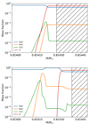 |
Fig. A.1. Chemical profiles of one of the hot TDUs in our 4 M⊙ model with advective mixing. Top: Prior to the deepest extent of the TDU. Bottom: Afterwards. The uninhibited effective C13 source is clear in this case. |
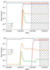 |
Fig. A.2. Same as Fig. A.1, but with a diffusive mixing. In this case the coupling of mixing and burning through operator splitting inhibits the C13 neutron source by placing the C13 pocket inside of the N14 pocket. |
Appendix B: Relevant data
Observed values reported by Abia et al. (2001, 2002) for the seven solar metallicity stars that we compare with our values in this work.
All Tables
TP average of the effective 13C pocket mass extent for each of the models presented here.
Average of [Y/Fe] and [Ce/Fe] as well as ratio [Ce/Y] by mass and overshoot parameter, ω, from our simulations.
Observed values reported by Abia et al. (2001, 2002) for the seven solar metallicity stars that we compare with our values in this work.
All Figures
|
Fig. 1. Abundance profiles resulting from overshoot mixing using Eq. (15) with the parameters ω = 0.10 (dashed) and ω = 0.14 (solid) for a 4 M⊙ case. Not only does the extent of the overshot region grow with the increase in the free parameter, but the slope of the proton profile decreases, which results in wider effective 13C pockets. The convective envelope is shown as the hatched area. |
| In the text | |
|
Fig. 2. L1 error (sum of the absolutes of the differences) for a chosen species and process when changing the number of steps n = {1, 2, 4, 8, 16} for each solver for the current NuPPN implementation. Each solution is compared to the solution yielded by the BD solver for n = 32 steps with a tolerance of 10−3. Left panel: final abundance for 16O in a 12 M⊙ He-burning trajectory. Right panel: final abundance for 138Ba for a 13C pocket trajectory. The BD and PED converge to the same solution. The slower convergence of the BE solver is due to its lower convergence order. |
| In the text | |
|
Fig. 3. Comparison of the time it takes for each solver to compute a solution for a 13C pocket trajectory. Top panel: time in absolute seconds. Lower panel: all the times normalised to the BE times. It is worth noting that even if BE is faster than BD, BE is less accurate for the same time steps, as shown in Fig. 2. The PED method is faster than the other two in all cases. |
| In the text | |
|
Fig. 4. Evolution of the He intershell 12C mass fraction during each of the TDU events represented in Tables 1–3. |
| In the text | |
|
Fig. 5. Evolution of the effective 13C pocket in the 3, 4, and 5 M⊙ stars for the overshoot parameters ω = 0.10, 0.12, and 0.14. The y axis shows the mass fraction of effective 13C as defined in Eq. (1), while the x axis shows the width of the pockets in solar masses, with each pocket representing the widest mass extent of the effective 13C pocket in each inter-pulse. This occurs once the protons have burned completely in the He intershell but before the 13C starts to burn. The pockets are artificially arranged, with the earliest inter-pulse to the left to the latest on the right, to show the temporal evolution of their shape and size. There is not a one-to-one correspondence of the number of 13C pockets presented here and the number of TP shown in Fig. 4. This is because a higher ω forces a higher TDU efficiency, forming more 13C pockets. |
| In the text | |
|
Fig. 6. Final stellar surface abundances of the elements heavier than Fe for the 3, 4, and 5 M⊙ ATON stars (top, middle, and bottom panel, respectively), post-processed with SNUPPAT with three different convective overshoot parameters, ω. The elements marked in red are those most sensitive to the neutron density. The breaks in the abundance distribution are due to the unstable isotopes Tc (Z = 43) and Pm (Z = 61). |
| In the text | |
|
Fig. 7. Comparison of s-process nucleosynthesis results on the stellar surface of 3 M⊙ models at solar metallicity of Monash, FRUITY, NuGrid, and SNUPPAT. From Monash, we selected the Z = 0.14 model with Mmix equal to 2 × 10⁻³ M⊙ (Karakas 2014; Karakas & Lugaro 2016). From the FRUITY models, we selected the Z = 0.014 and Z = 0.02 models. From NuGrid, we chose the Z = 0.02 models from Battino et al. (2016), marked in the legend as ‘B16’, and Pignatari et al. (2016), marked in the legend with ‘P16’. |
| In the text | |
|
Fig. 8. Same as Fig. 7, but for 4 M⊙ models, except that we halve the value of Mmix for the Monash model. |
| In the text | |
|
Fig. 9. Same as Fig. 7 but for 5 M⊙ models, except that we include Monash models with Mmix of 10−4 M⊙ and 0. We have also included a model with ω = 0.12 for SNUPPAT and removed one of the FRUITY models for clarity. |
| In the text | |
|
Fig. 10. Observed [s/Fe] and [hs/ls] ratios for solar metallicity C stars from Abia et al. (2001, 2002) alongside the evolution of ratios for the 3 M⊙ models. The red squares are stars with ‘doubtful’ Tc detection. The blue inverted triangles are stars with bolometric magnitude lower than −5.5, which should correspond to the more massive among the sample, closer to our 3 M⊙ simulations. The black triangles are stars with bolometric magnitude higher than −5.5 and Tc detection. The uncertainties are those given in Abia et al. (2001, 2002). |
| In the text | |
|
Fig. 11. Observed abundances from Madonna (2018) of PN NGC 3918 (open triangles) and NGC 7027 (filled squares) alongside the best fitting of our overabundance results (lines and filled dots). In grey are shown the uncertainties for each of the measurements. |
| In the text | |
|
Fig. A.1. Chemical profiles of one of the hot TDUs in our 4 M⊙ model with advective mixing. Top: Prior to the deepest extent of the TDU. Bottom: Afterwards. The uninhibited effective C13 source is clear in this case. |
| In the text | |
|
Fig. A.2. Same as Fig. A.1, but with a diffusive mixing. In this case the coupling of mixing and burning through operator splitting inhibits the C13 neutron source by placing the C13 pocket inside of the N14 pocket. |
| In the text | |
Current usage metrics show cumulative count of Article Views (full-text article views including HTML views, PDF and ePub downloads, according to the available data) and Abstracts Views on Vision4Press platform.
Data correspond to usage on the plateform after 2015. The current usage metrics is available 48-96 hours after online publication and is updated daily on week days.
Initial download of the metrics may take a while.