| Issue |
A&A
Volume 697, May 2025
|
|
|---|---|---|
| Article Number | A48 | |
| Number of page(s) | 18 | |
| Section | Stellar structure and evolution | |
| DOI | https://doi.org/10.1051/0004-6361/202453089 | |
| Published online | 05 May 2025 | |
Impact of T- and ρ-dependent decay rates and new (n,γ) cross-sections on the s process in low-mass asymptotic giant branch stars
1
Department of Experimental Physics, Institute of Physics, University of Szeged, H-6720 Szeged, Dóm tér 9, Hungary
2
Konkoly Observatory, HUN-REN CSFK/RCAES, Konkoly Thege Miklós út 15-17, H-1121 Budapest, Hungary
3
CSFK, MTA Centre of Excellence, Konkoly Thege Miklós út 15-17., H-1121 Budapest, Hungary
4
Computer, Computational and Statistical Sciences (CCS) Division, Center for Theoretical Astrophysics, Los Alamos National Laboratory, Los Alamos, NM 87545, USA
5
School of Physics and Astronomy, Monash University, VIC 3800, Australia
6
ARC Centre of Excellence for All Sky Astrophysics in 3 Dimensions (ASTRO 3D), Clayton, VIC 3800, Australia
7
ELTE Eötvös Loránd University, Institute of Physics and Astronomy, Pázmány Péter sétány 1/A, Budapest 1117, Hungary
⋆ Corresponding author: This email address is being protected from spambots. You need JavaScript enabled to view it.
Received:
20
November
2024
Accepted:
1
March
2025
Abstract
Aims. We study the impact of nuclear input related to weak-decay rates and neutron-capture reactions on predictions for the slow neutron-capture process (s process) in asymptotic giant branch (AGB) stars. We provide the first database of surface abundances and stellar yields of the isotopes heavier than iron from the Monash models.
Methods. We ran nucleosynthesis calculations with the Monash post-processing code for seven stellar structure evolution models of low-mass AGB stars with three different sets of nuclear inputs. The reference set has constant decay rates and represents the set used in the previous Monash publications. The second set contains the temperature and density dependence of β decays and electron captures based on the default rates of nuclear NETwork GENerator (NETGEN). In the third set, we further update 92 neutron-capture rates based on re-evaluated experimental cross sections from the ASTrophysical Rate and rAw data Library. We compare and discuss the predictions of the sets relative to each other in terms of isotopic surface abundances and total stellar yields. We also compare the results to isotopic ratios measured in presolar stardust silicon carbide (SiC) grains from AGB stars.
Results. The new sets of models result in a ∼66% solar s-process contribution to the p-nucleus 152Gd, confirming that this isotope is predominantly made by the s process. The nuclear input updates result in predictions for the 80Kr/82Kr ratio in the He intershell and surface 64Ni/58Ni, 94Mo/96Mo, and 137Ba/136Ba ratios that are more consistent with the corresponding ratios measured in stardust; however, the new predicted 138Ba/136Ba ratios are higher than the typical values of the SiC grains. The W isotopic anomalies are in agreement with data from the analyses of other meteoritic inclusions. We confirm that the production of 176Lu and 205Pb is affected by too large uncertainties in their decay rates from NETGEN.
Key words: nuclear reactions / nucleosynthesis / abundances / methods: numerical / stars: AGB and post-AGB
© The Authors 2025
 Open Access article, published by EDP Sciences, under the terms of the Creative Commons Attribution License (https://creativecommons.org/licenses/by/4.0), which permits unrestricted use, distribution, and reproduction in any medium, provided the original work is properly cited.
This article is published in open access under the Subscribe to Open model. This email address is being protected from spambots. You need JavaScript enabled to view it. to support open access publication.
1. Introduction
At the end of their lives, low-mass stars (1 M⊙ ≲ M ≲ 8 M⊙) evolve to the asymptotic giant branch (AGB, Iben & Renzini 1983; Busso et al. 1999; Herwig 2004; Karakas & Lattanzio 2014). AGB stars are characterised by a degenerate C-O core, a H and a He shell, and an extensive, convective, H-rich envelope. The two shells are separated by a thin He-rich layer called the intershell. The energy production occurs in cycles: a relatively long phase of H burning is periodically (every ∼103–105 years, depending on the stellar mass) interrupted by a thermal instability of the He shell, which is called a thermal pulse (TP, Schwarzschild & Härm 1965; Weigert 1966). The rapid release of a substantial amount of energy during a TP causes the development of a convective region in the intershell, hereafter referred to as a ‘convective pulse’, and the star to expand from the He shell outward. This expansion allows the envelope to extend downwards after the extinction of the convective pulse, potentially penetrating the intershell region and carrying material from there to the surface. The resulting mixing episodes are collectively referred to as the third dredge-up (TDU). The intershell material carried to the stellar surface contains a large amount of carbon produced by partial He burning; therefore, the TDU can convert the surface layers of the AGB star to evolve from being oxygen-rich to being carbon-rich (C/O ≥ 1, Wallerstein & Knapp 1998). The cycle described above is repeated several times (tens to hundreds of times, depending on the initial mass) before the envelope is completely eroded by mass loss, and the C-O core of the star is left as a white dwarf.
In the thermally pulsing AGB phase, conditions are suitable for (α,n) neutron-source reactions to be initiated in the intershell. The 22Ne(α, n)25Mg reaction (Cameron 1960; Truran & Iben 1977) is activated for temperatures greater than 300 MK during the convective pulses of AGB stars with an initial mass greater than ∼3 M⊙ and results in a high maximum neutron density (∼1013 n cm−3, e.g. Fishlock et al. 2014) but a low total amount of free neutrons. The 13C(α, n)16O reaction (initially reported by Hollowell & Iben 1988) is activated during the H-burning phase, at T ∼ 90 MK and results in a high total amount of free neutrons but a low maximum neutron density (∼107 n cm−3, Straniero et al. 1995). The captures of the resulting free neutrons drive slow neutron captures; that is, the s process (Burbidge et al. 1957; Käppeler et al. 2011; Lugaro et al. 2023b), which produces roughly half of the abundances of elements heavier than iron (up to lead) in the Universe (see review by Lugaro et al. 2023b).
During the s process, by definition, the probability of neutron capture on an unstable isotope is lower than its decay; therefore, the main neutron-capture path follows the valley of β-stability. However, depending on the temperature, density, and neutron density, the neutron-capture rate of some unstable isotope may compete with their decay rate. These unstable isotopes are known as branching points on the s-process path (e.g. Bisterzo et al. 2015; Lugaro & Chieffi 2018). The branching factor, fβ, is defined as:
 (1)
(1)
where fn is the branching factor of the neutron capture channel, λβ is the β-decay rate (λβ = ln2  , where t1/2 is the half-life), and λn = Nn ⟨σv⟩ is the neutron-capture rate given by the neutron density, Nn, the relative velocity of neutrons and target nuclei, v, and the neutron capture cross section, σ. The ⟨σv⟩ can be approximated as the product of the Maxwellian-average cross section (MACS or σM) and the thermal velocity, vth.
The calculation of fβ is not trivial because not only Nn varies; λβ and σM can also change with T and ρ. Neutron-capture rates on a nucleus ground state do not significantly vary with temperature; however, to obtain neutron-capture rates in a stellar environment, in addition to laboratory ground-state cross sections, the theoretical relative contribution of excited states (Rauscher 2012), generally described using a stellar enhancement factor (SEF), needs to be included. Also, laboratory β-decay rates can be largely modified at stellar temperatures due to the thermal population of low-lying excited states, which may have different β-decay lifetimes (e.g. Reifarth et al. 2018a). In addition, temperature and electron density change the population of electronic states, providing the possibility of the bound-state decay (Bahcall 1961). Electron-capture rates are also influenced by temperature and electron density: the likelihood of a bound electron near the nucleus decreases with temperature, while the probability of a free electron near the nucleus increases with electron density (e.g. Takahashi & Yokoi 1987). Accounting for these effects is essential for the accurate modelling of the s process in AGB stars.
Here, we present a major upgrade of nuclear reaction rates of the Monash nucleosynthesis code. We replaced the constant radioactive-decay and electron-capture reactions with T- and ρ-dependent tables. The tables were based on the compilation of NETGEN (nuclear NETwork GENerator, Jorissen & Goriely 2001; Aikawa et al. 2005; Xu et al. 2013). Most other sets of models – NuGrid (Nucleosynthesis Grid, e.g. Pignatari & Herwig 2012), FUNS (FUll Network Stellar, e.g. Straniero et al. 2006), and STAREVOL (e.g. Siess 2006) – have already implemented T- and ρ-dependent decay rates and provided the resulting yields and abundances. However, the thorough analysis that we present here regarding the impact of using variable weak rates on the activation of branching points and the implications on the comparison with observations, including the interpretation of stardust grain data, is still missing from the literature. To our knowledge, recently only Bisterzo et al. (2015) have presented a detailed analysis of branching points, but from the point of view of the impact of the uncertainties of the neutron source reactions. Furthermore, we include new tabulated neutron-capture rates for 92 reactions using re-evaluated experimental MACSs from the ASTRAL database (ASTrophysical Rate and rAw data Library, Reifarth et al. 2018b; Vescovi & Reifarth 2021; Vescovi et al. 2023) and SEFs from KaDoNiS (Karlsruhe Astrophysical Database of Nucleosynthesis in Stars, Dillmann et al. 2006). We provide the first database of surface abundances and stellar yields of the isotopes heavier than iron from the Monash models.
The paper is organised as follows. We start with a description of our methods and of the seven stellar evolutionary models used for the post-processing nucleosynthesis calculations (Sect. 2). In Sect. 3, we present the impact of nuclear input changes on nucleosynthesis predictions and discuss the results including a comparison to other studies and a selection of isotopic ratios measured in presolar stardust silicon carbide (SiC) grains from AGB stars. The conclusions are provided in Sect. 4.
2. Methods and models
We provide predictions for stellar abundances from AGB stars, using the Monash post-processing nucleosynthesis code (Cannon 1993), which calculates the changes in the abundances of currently 328 nuclear species due to convective mixing and nuclear burning on the basis of detailed stellar structure calculated by the Monash evolution code (Lattanzio 1986; Karakas 2014). In summary, the current nuclear reaction network of the nucleosynthesis code includes 2351 reactions, most of which are based on the JINA reaclib database (Cyburt et al. 2010), where reaction rates are expressed as a function of temperature T9 (in units of 109 Kelvin) using a seven-parameter (a0 − 6) analytical formula (Thielemann et al. 1986):
![Mathematical equation: $$ \begin{aligned} \lambda = \mathrm{exp} \left[a_0 + \sum _{\mathrm{i} = 1}^{5} a_{\mathrm{i} }\,T_9^{\frac{2\mathrm{i} -5}{3}} + a_6\,\mathrm{ln} T_9\right]. \end{aligned} $$](/articles/aa/full_html/2025/05/aa53089-24/aa53089-24-eq3.gif) (2)
(2)
While the JINA reaclib database is advantageous for building a large network, it has two major disadvantages: (1) For some experimental rates, there can be a variation of up to 10%–20% of the fit from the actual rate. (2) The β-decay and electron-capture rates are constant; that is, they do not depend on temperature and electron density. For these reasons, a new version of the nucleosynthesis code was developed by van Raai et al. (2012), which includes a routine that allows us to use specific reaction rates as tabulated values instead of the reaclib fit, and here it was extended to decay rates.
2.1. Stellar models
As input for post-processing nucleosynthesis calculations, we used a selection from the stellar structure evolution models presented in Karakas (2014) and Karakas & Lugaro (2016). We selected M = 2, 3, 4 M⊙, Y = 0.28 stellar models of solar metallicity (Z = 0.014, based on the solar abundances from Asplund et al. 2009), M = 3, 4 M⊙, Y = 0.26 stellar models at half-solar metallicity (Z = 0.007), and M = 3, 4 M⊙, Y = 0.30 stellar models at double-solar metallicity (Z = 0.03)1. Input physics and methodology of the stellar structure models are described in full in the papers mentioned above. In summary, mass loss was not included in the red giant branch (RGB) phase and the mass-loss rate of Vassiliadis & Wood (1993) was used in the AGB phase. The models used the mixing length theory of convection with a mixing-length parameter α = 1.86. The convective overshoot was not included in the calculations except for the 3 M⊙Z = 0.03 model, where an overshoot parameter (Nov = 1) was used which resulted in a C-rich star.
Table 1 shows some relevant properties of the calculated AGB models. (1) The total number of TDUs increases with increasing initial stellar mass. (2) The number of TPs during which the envelope is C-rich depends also on the mass, the mass loss, and the activation of hot bottom burning (i.e. H-burning at the base of the envelope) in the 4 M⊙ stars. (3) The maximum temperature reached during TPs, which controls the activation of the 22Ne(α, n)25Mg neutron source increases with increasing stellar mass and decreasing metallicity.
Relevant features of the stellar models grouped by metallicity.
2.2. Post-processing calculations
The operation of the 13C(α, n)16O neutron source requires the formation of a partial mixing zone (PMZ), where protons from the convective envelope are mixed with the intershell matter and captured by the abundant 12C, resulting in the so-called 13C pocket (Straniero et al. 1997; Gallino et al. 1998; Goriely & Mowlavi 2000). Our method of including the 13C pocket is described in detail in Karakas & Lugaro (2016). In summary, protons are partially mixed at the end of each TDU down to a mass extent in the intershell denoted by MPMZ, using an exponential profile. At the top of the intershell (corresponding to the base of the envelope during the TDU), the abundance of protons Xp is that of the envelope, while at MPMZ in the intershell it is Xp = 10−4. Below this mass point, Xp = 0. Different MPMZ values as functions of the stellar mass are defined and justified by Karakas & Lugaro (2016) and Buntain et al. (2017). Here, we used the ‘standard’ values reported in Table 1.
We ran post-processing nucleosynthesis calculations with three different inputs (see Table 2) for the nuclear network. The original set (hereafter Set 0) contains nuclear reactions mostly from the JINA reaclib database. The neutron-source reactions 13C(α, n)16O and 22Ne(α, n)25Mg are from Heil et al. (2008a) and Iliadis et al. (2010), respectively. For neutron capture reactions, Set 0 uses the ka02 labelled fits of JINA reaclib, which are based on the KaDoNiS database, except for Zr isotopes, whose rates are from Lugaro et al. (2014a), and for a few other isotopes, whose rates are taken directly from KaDoNiS. These were selected because the JINA fit did not accurately cover the KaDoNiS data. This is the same network used by Karakas & Lugaro (2016), except that in Set 0 we updated the temperature dependence of the β-decay rate of 134Cs from Takahashi & Yokoi (1987) used in Karakas & Lugaro (2016) to Li et al. (2021) and of 181Hf from Lugaro et al. (2014b), which was included as terrestrial constant in Karakas & Lugaro (2016).
Sources of the reaction rates in the different sets.
In the second set (hereafter Set 1), we implemented the temperature and density dependence of β-decays and electron captures in the network using the default (most recent) rates from the NETGEN library. Below mass number A = 56, the rates are based on Horiguchi et al. (1996), except for the β−-decay rate of 48Ca, which is based on Langanke & Martínez-Pinedo (2000), and the electron-capture rates of 7Be and 36Cl, which are based on Caughlan & Fowler (1988) and Oda et al. (1994), respectively. Above A = 56, the rates are based on the nominal rates of Goriely (1999), while the reactions not included in Goriely (1999) are based on Takahashi & Yokoi (1987), except for the β−-decay rate of the excited 85Kr isomer, which is based on Horiguchi et al. (1996). In addition, we extend the reaction list by including the bound-state β decay of the terrestrial stable 205Tl based on Goriely (1999). Most of our decay tables contain the values in a grid of 250 temperature points between 1 MK and 1 GK on a logarithmic scale. For the rates that also depend on the electron density, the NETGEN tables consist of data in the same temperature grid as above for four electron densities: 1, 3, 9.5 or 10 (depending on the reference), and 30 × 1026 cm−3, except for 36Cl and 48Ca, which include data for 11 electron density points between 6 × 1024 and 6 × 1033 cm−3. We tested the possible effect of the choice of temperature grid on the M = 3 M⊙, Z = 0.014 model. We found that the application of a looser grid (125 points) or a finer grid (300 points) results in the same abundances within 1%, except for 204Pb, 205Pb, and 205Tl, which changed by less than 10%.
In the third set (hereafter Set 2), we upgraded the neutron-capture rates of 92 reactions using re-evaluated experimental MACSs from the ASTRAL database and SEFs from KaDoNiS v0.3. The current version (v0.2) of ASTRAL includes MACSs for 122 isotopes based on time-of-flight measurements, which have been re-evaluated by taking into account the new recommended value for the gold differential cross section (Reifarth et al. 2018b) and 50 isotopes whose experimental cross section data are based on activation measurements (Vescovi et al. 2023). The neutron-capture rates at each temperature are calculated as λn = (NA σM vth) × SEF, where NA = 6.02 × 10²³ is the Avogadro constant.
2.3. Surface abundances, stellar yields, and δ values
The nucleosynthesis code provides us with the time-evolution of normalised number abundances,  , of each isotope i at the surface of the model stars. Using these outputs, we can calculate the total stellar yield, Mi, as the total mass of each isotope, i, expressed in unit of solar mass, ejected into the interstellar medium (ISM) during the entire life of the star. To do this, we used an approximate formula, which sums over all the TPs (instead integrating over the entire lifetime of the star) the mass lost for each isotope in-between each TP (identified by the index, k) according to:
![Mathematical equation: $$ \begin{aligned} M_{\mathrm{i} } = \left[ \sum ^{final}_{k = 1} \left( M_{\mathrm{k-1} } - M_{\mathrm{k} } \right) X^{\mathrm{i} }_{\mathrm{k} } \right] + \left( M_{\mathrm{final} } - M_{\mathrm{core} } \right) X^{\mathrm{i} }_{\mathrm{final} }, \end{aligned} $$](/articles/aa/full_html/2025/05/aa53089-24/aa53089-24-eq7.gif) (3)
(3)
where Mk is the mass of the model star at the end of TP k,  =
=  is the surface abundance of isotope i in the mass fraction at the end of same TP k (where mi is the atomic mass of isotope i), and Mfinal and Mcore are, respectively, the total mass and the core mass at the end of the computed evolution (i.e. when the code stops converging). The second term of the equation was added to remove the full envelope, assuming that no more TDU happens. We provide
  and Mi for all our models as Online Material. We note that this approximated formula works here because the models we consider do not have any mass loss on the RGB and we tested that our Set 0 yields are within 2% of those published by Karakas & Lugaro (2016).
While stellar yields are an important input for the Galactic chemical evolution (GCE) calculations (e.g. Côté et al. 2019; Trueman et al. 2022), isotopic abundance ratios are needed to interpret the composition of presolar stardust grains, such as SiC grains found in meteorites. Most of the SiC grains condensed in carbon-rich AGB stellar winds and were ejected into the ISM (Zinner 2014). The grains were transported to the protosolar nebula, trapped within the parent bodies of meteorites, which delivered them to Earth where they can be extracted and analysed in the laboratory (e.g. Bernatowicz et al. 1987; Lewis et al. 1990). The Presolar Grain Database (PGD, Hynes & Gyngard 2009; Stephan et al. 2024) contains all the available isotope data for single presolar stardust SiC grains. To compare to the SiC grain data, we calculated the isotopic ratios of each element in the form of δ values: that is, per mil variations with respect to the solar ratio as:
 (4)
(4)
where i, j represents the isotopes of element E at the end of TP k. The solar abundances in this case are also based on Asplund et al. (2009).
3. Results and discussion
3.1. Comparison of Set 1 to Set 0
In this section, we compare the predictions of the Set 0 and Set 1 models using the final surface normalised number abundances,  , of the model stars. There are 30 isotopes whose abundance changed by at least 10% in at least one Set 1 stellar model compared to the corresponding Set 0 stellar model. The list of these isotopes and their YSet 1, finali/YSet 0, finali ratio are shown in Table A.1. The abundances of individual isotopes, in addition to the nuclear input, depend on the characteristics of the stellar models (e.g. temperature, electron and neutron density, number of mixing episodes) and therefore the effects of the new rates can differ greatly between models. In the following, we present the most relevant isotope cases.
Table A.2 highlights the relevant information for each case, including the branching isotopes, the decay modes and decay rates of the corresponding isotopes, the direction in which the abundance of each isotope has changed in the Set 1 models compared to Set 0 models, and the relevance of each case.
3.1.1. 64Ni
The s-process production of 64Ni depends on the operation of the 63Ni and 64Cu branching points. 63Ni suffers β− decay with a laboratory half-life of 99.8 yr producing 63Cu. According to NETGEN, the β−-decay rate of 63Ni increases by roughly an order of magnitude from the terrestrial value under the conditions that prevail in the intershell (see Table A.2). As is shown in Eq. (1), the probability of neutron capture decreases with increasing decay rates; therefore, we obtain a lower 64Ni abundance from this channel in Set 1 models than in Set 0 models. The isotope 64Cu, with a half-life of 12.8 hours, can both β− and β+ decay, where the latter channel is twice as fast compared to the β− under terrestrial conditions. While the rate of the β− channel of 64Cu slightly increases with T, the β+-decay rate is instead reduced by about a third at 300 MK. The probability of the β+ channel also decreases with electron number density. These effects also contribute to the decrease in the amount of 64Ni in Set 1 models. In total, we obtain 1% to 12% less 64Ni in the final stage of the Set 1 models compared to Set 0. For nickel, a large number of SiC grain data are available following the work of Trappitsch et al. (2018); therefore, we compare the predictions of our models with these data in Section 3.3.1.
3.1.2. 80, 81Kr
The s-process production of the stable 80Kr and the unstable 81Kr with a half-life of 229 kyr depends on the operation of the 79Se and 80Br branching points. 79Se suffers β− decay with a laboratory half-life of 297 kyr producing 79Br. Neutron captures on 79Br produce unstable 80Br with a half-life of 17.7 minutes. 80Br can both β− and β+ decay, the former channel being almost ten times faster than the latter and resulting in the production of 80Kr. From 80Kr, 81Kr can be produced by neutron captures, in addition to its amount also depending on its own electron capture rate. Comparing the final surface abundances of the Set 1 models with those of Set 0, we obtain 1.94–4.65 times more 80Kr and 7.23–344.43 times more 81Kr. We note that the abundance of 82Kr also increases slightly, by 2–15%. All these changes are mainly due to the operation of the 79Se branching point, whose decay rate increases by orders of magnitude under stellar conditions (Table A.2). We note that a measurement-based T- and ρ-dependent half-life of 79Se is available (Klay & Käppeler 1988). The half-life from NETGEN is within 10% of the half-life of Klay & Käppeler (1988) over the whole temperature range.
Krypton is a noble gas. It does not condense into dust, but it can be ionised and implanted into the grains (Verchovsky et al. 2004). In fact, the isotopic composition of trace amounts of Kr in SiC grains shows the signature of mixing of pure s process and solar composition material. Lewis et al. (1994) analysed the isotopic composition of Kr in bulk samples of a million SiC grains from the Murchison KJ series (Amari et al. 1994) and used linear regression to derive the isotopic composition of Kr in the intershell of AGB stars. They found that the isotopic ratios vary with grain size (the 80Kr/82Kr ratio decreases with grain size), suggesting that these SiC grains came from stars of different masses and metallicities.
Table 3 shows the 80Kr/82Kr ratios in the intershell of the Set 0 and Set 1 models before the last TDU episode. We compare only the solar and double-solar metallicity model predictions with the Lewis et al. (1994) data because the vast majority (> 90%) of SiC grains, the mainstream (MS) grains, are believed to originate in low-mass C-rich AGB stars with around solar (Hoppe et al. 1994), slightly super-solar (Lewis et al. 2013), and double-solar (Lugaro et al. 2020) metallicity. Also, recent results by Cristallo et al. (2020) suggest that the stardust SiC grains predominantly came from AGB stars around M = 2 M⊙ and Z = 0.014. For most of the Set 0 models, this ratio is an order of magnitude lower than the range of Lewis et al. (1994); for the M = 4 M⊙Z = 0.014 model, this difference is even greater. In contrast, the 80Kr/82Kr ratios derived by the Set 1 models are of the same order of magnitude as the possible intershell ratios; in addition, the predictions of three Set 1 models are within the range observed. We note that a new 80Kr(n, γ) cross section is available following the work of Tessler et al. (2021). When testing on M = 2 and 3 M⊙Z = 0.014 models, the new neutron-capture rate of 80Kr based on Tessler et al. (2021) results in slightly higher (up to 13%) 80Kr/82Kr ratios and does not change our conclusions above.
80Kr/82Kr ratios in the selected Set 0 and Set 1 models and for each KJ fraction.
3.1.3. 94Mo
By definition, stable proton-rich isotopes that cannot be reached by neutron-capture processes are p-only isotopes (or the p-nuclei, Cameron 1957). The p-only 94Mo can also be produced via the s process by two consecutive neutron captures on 92Mo and the operation of 93Zr and 94Nb branching points. 94Mo is the daughter nucleus of 94Nb. The latter can be produced by neutron captures on both the initial amount of stable 93Nb and the small fraction of 93Nb that comes from the β−-decay of 93Zr. 92Mo is also a p-nucleus and it cannot be produced by the s process under any circumstances. The 92, 93Mo isotopes are not included in our network; therefore, the 92Mo(n, γ)93Mo(n, γ)94Mo channel is also missing. However, we tested that its impact on the abundance of 94Mo is typically less than ∼1%. Although the decay rate of 93Zr increases slightly with temperature and electron density, the decay rate of 94Nb is six orders of magnitude higher in the intershell region of AGB stars than under terrestrial conditions (see Table A.2). Therefore, while more 94Nb is produced in the Set 1 models compared to Set 0, its abundance also decays much faster, leading to a decrease in the final surface abundance by orders of magnitude and a milder increase (at most 53%) in the abundance of 94Mo.
Several publications have analysed the isotopic compositions of molybdenum in SiC grains (e.g. Nicolussi et al. 1998; Lugaro et al. 2003; Stephan et al. 2019). As was shown in these previous studies, the isotope ratios observed in SiC grains show the mixtures of pure s-process matter with solar material. In addition, the δ94Mo96 values are correlated with the δ92Mo96 values, and the slope of the regression line indicates the presence of a small s-process contribution to 94Mo. We calculated the linear regression2 of δ values from Barzyk (2007), Liu et al. (2017b, 2019) and Stephan et al. (2019) and we obtained an intercept of δ94Mo96 = −961.8‰ ± 1.2‰ at δ92Mo96 = −1000‰, which is consistent with the result of Stephan et al. (2019). We can estimate the s-process contribution, si, for 94Mo from our models using the following equation:
 (5)
(5)
where  is the weighted mean yield (see below) of isotope i obtained by our stellar models normalised to the unbranched s-only isotope 150Sm, whose solar abundance and neutron capture cross section are known with high precision (Gallino 2023). The weighted mean yields were calculated with a trapezoidal rule quadrature with a constant mass interval:
 (6)
(6)
where j indicates the mass in question. The weight is based on the Salpeter initial mass function (IMF, Salpeter 1955), used here to mimic the yields for the entire AGB stellar population. Our prediction for the s-process contribution of 94Mo does not change significantly: it slightly increases from 0.034 to 0.04 from Set 0 to Set 1, and both are consistent with ∼0.038 coming from the data regression (see also Stephan et al. 2019).
In addition, we can compare the surface evolution of each model with the grain data. For an easier comparison to model predictions, in Fig. 1 we plot the logarithms of the ratio of the isotopes i and j at each TP k normalised to solar composition using standard astrophysical notation:
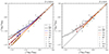 |
Fig. 1. [94Mo/96Mo] vs [92Mo/96Mo] from SiC grain data as dark grey circles MS grains and downward and upward triangles for Y and Z grains, respectively, with 1σ error bars (from Barzyk 2007; Liu et al. 2017b, 2019; Stephan et al. 2019) compared to the surface evolution of Set 0 and Set 1 stellar models of solar (left panel) and of double-solar metallicity (right panel) of different masses (see legend). Circles (Set 0) and triangles (Set 1) on the lines represent the composition after each TDU after the envelope becomes C-rich. The solid black line represents the linear regression from δ94Mo96 vs δ92Mo96, while the dashed black line represents the [94Mo/96Mo] = [92Mo/96Mo] line. |
![Mathematical equation: $$ \begin{aligned}{[{\ }^{\mathrm i}E/^{j}E]} = \log (Y^{\mathrm{i} }/Y^{\mathrm{j} })_{\mathrm{sample} } - \log (Y^{\mathrm{i} }/Y^{\mathrm{j} })_{\rm \odot }. \end{aligned} $$](/articles/aa/full_html/2025/05/aa53089-24/aa53089-24-eq16.gif) (7)
(7)
As in the case of 80Kr, we only use the predictions of the solar and double-solar metallicity models, but include the few data points available for grains from the minor Y and Z populations, believed to have originated in stars of sub-solar metallicity, because in Fig. 1 these grains plot in the same region as the MS grains. The two 4 M⊙ models are on the 1:1 line regardless of the choice of the reaction rates, which means that the 94Mo production is not relevant in these stars; therefore, they do not represent the majority of the grain parent stars, especially in the case of the solar metallicity model (Lugaro et al. 2018a). On the other hand, the surface evolution of the 2 and 3 M⊙ Set 1 models closely follows the regression line. Most previous models (e.g. Arlandini et al. 1999; Lugaro et al. 2003; Bisterzo et al. 2014; Liu et al. 2019) were unable to produce enough 94Mo to match the grain data, our new models resolve this problem. Models in FRUITY (FUll-Network Repository of Updated Isotopic Tables & Yields, e.g. Cristallo et al. 2009, 2011, 2015) also produce a significant amount of 94Mo, actually resulting in values lying even above the line defined by the grains (Vescovi et al. 2020). Therefore, we conclude that the previous mismatch was likely due to inaccurate nuclear input data and/or treatment of the branching points, which was updated in the past decade or so in the new generation of AGB nucleosynthesis models.
3.1.4. 108Cd
The case of 108Cd is similar to 94Mo: it is a p-nucleus with a small s-process contribution. It can be produced via s process by the β−-decay of 108Ag, which can be produced by neutron captures on the initial amount of 107Ag and the small fraction that comes from the β−-decay of 107Pd. 108Ag can both β− and β+ decay with a relatively short half-life (2.4 min). The β− channel does not depend significantly on temperature and density and is faster than the β+ channel under both stellar and terrestrial conditions (see Table A.2). In contrast, the β−-rate of 107Pd increases by orders of magnitude with temperature, causing the amount of 108Cd to increase by 2-64% in the Set 1 models with respect to the Set 0 models. We estimate the s-process contribution for 108Cd according to the method used for 94Mo. As in the case of 94Mo, our predictions of the two sets are quite close: the estimated s-process contribution of the solar 108Cd abundance increases slightly from 0.04 to 0.048 from Set 0 to Set 1.
3.1.5. 129I
The small s-process production of r-only 129I depends on the β− decay of 128I. By definition, species that cannot be produced by the s process due to an unstable nucleus that precedes them on the s-process path are traditionally r-only isotopes. In fact, no isotope is completely shielded against s-process production, nuclei on the neutron-rich side of the β-stability valley can have a low s contribution, depending on the activation of branching points (Bisterzo et al. 2015). In addition, 129I is a so-called short-lived radionuclide (SLR, a radioactive isotope with a half-life between about 0.1 to 100 million years, see, e.g. Lugaro et al. 2018b); therefore, its amount depends also on its decay. Neither the decay of 128I nor that of 129I is significantly dependent on the electron density, but the β−-decay rate of 128I decreases slightly with temperature, while the decay rate of 129I increases by orders of magnitude with temperature (see Table A.2). While we produce more 129I from this channel in the Set 1 models than in the Set 0 models, its final amount decreases by up to an order of magnitude due to its shorter half-life at stellar temperatures.
The presence of SLRs has been documented in the early Solar System (ESS) from the laboratory analysis of meteorites (e.g. Dauphas & Chaussidon 2011; Davis 2022). These nuclei have now decayed completely, but their ESS abundances can be inferred from measurable excesses in the abundances of their daughter nuclei. Therefore, we cannot determine the solar s-contribution, but we can calculate the so-called abundance production factor Ps; that is, the relative amount produced by the s process compared its stable reference isotope:
 (8)
(8)
where i represents the radioactive and j represents the stable isotope of the corresponding element. The 129I/127I production factors derived by our Set 0 and Set 1 models are 1 × 10⁻⁴ and 2.8 × 10⁻⁴, respectively. These values are similar to the previous Monash result (Ps ≃ 10−4, Lugaro et al. 2014b), based on AGB models with initial mass between 1.25 and 8.5 M⊙. These production factors are generally four magnitudes lower than the r-process production factor P(r) = 1.35 (Lugaro et al. 2014b; Côté et al. 2021), which confirms that the 129I contribution from the s process is very marginal.
3.1.6. 152Gd
The s-process production of 152Gd depends on the operation of the 151Sm and 152Eu branching points. 152Eu can capture electrons and undergo β− decay with a laboratory half-life of 13.3 yr. The rate of electron capture increases with both temperature and electron density, while the rate of the β− channel increases only with temperature. The amount of 152Eu produced is determined by the β−-decay of 151Sm, whose rate also increases with temperature depending on the electron density (see Table A.2). Comparing the Set 1 models to the Set 0 models, we produce more 152Eu, which is more likely to suffer β− decay under stellar conditions than under terrestrial conditions; therefore, we obtain ∼2–28 times more 152Gd, depending on the stellar model.
152Gd was one of the 35 original p-nuclei (Cameron 1957), but nowadays it is well accepted that it has a large s-process contribution (Arlandini et al. 1999; Bisterzo et al. 2011, 2014), or it is even considered as an s-only isotope (Travaglio et al. 2011). Arlandini et al. (1999) calculated s-process contributions using the arithmetic average yields of 1.5 and 3 M⊙ half-solar metallicity AGB models from Gallino et al. (1998) and normalised to solar abundances by Anders & Grevesse (1989). Bisterzo et al. (2011) updated their results, taking into account more recent neutron-capture cross sections and using solar abundances from Lodders et al. (2009) to normalise. The s-contribution for 152Gd is 0.883 and 0.705 in Arlandini et al. (1999) and Bisterzo et al. (2011), respectively. Bisterzo et al. (2014) obtained the s-components of the solar composition using the GCE code described by Travaglio et al. (2004) and s-process yields from AGB stellar models by Gallino et al. (1998). They predicted 0.865 for the s-contribution of 152Gd from low-mass AGB stars. We used the method described in Sect. 3.1.3 to obtain the s-contributions of 152Gd. Comparing the predictions of the Set 0 and Set 1 models shows that we need to accurately model the operation of the branching points to understand the nucleosynthesis origin of this isotope. In the Set 0 models, the solar s-contributions of 152Gd is only 0.072, which would lead us to conclude that 152Gd is produced mainly by the p process. In contrast, Set 1 models predict 0.658 solar s-contributions, which confirm that this isotope predominantly originates from low-mass AGB stars. This prediction is broadly consistent with recent results (Prantzos et al. 2018; Busso et al. 2021) and with the results presented above, especially with Bisterzo et al. (2011), whose method of calculating the s-process contributions was similar to ours, but used only two models. We emphasise that our method gives an approximate estimate, while the Bisterzo et al. (2014) results were based on a full GCE model, which is a more accurate approach because it includes many more models which are also of a much lower metallicity than the ones considered here, and evolves each star according to its mass and therefore lifetime.
3.1.7. 176Lu and 176Hf
The β−-decay rate of 176Lu is highly sensitive to temperature during TPs (Takahashi & Yokoi 1987; Klay et al. 1991; Doll et al. 1999) due to the coupling of the very long-lived ground state (t1/2 = 37.9 Gyr) and the short-lived isomer (t1/2 = 3.7 h) at 123 keV via a thermal population of mediating states at higher energies, in particular at E = 838.6 keV, since direct transition is forbidden by selection rules. The high T dependence affects the abundance ratio of 176Lu and its daughter nucleus 176Hf in AGB stars, which must match the relative solar abundances of these isotopes, since both isotopes are s-only, shielded by 176Yb against r-process production. In other words, these isotopes must have the same overabundances as 150Sm; that is, their s-contributions must be close to 1. A minor deviation in the s-contribution (1.05 ± 0.05 for 176Lu and 1 ± 0.05 for 176Hf) is acceptable (Heil et al. 2008b) due to the β− decay of 176Lu in the ISM.
The discrepancy between the theoretical and observed 176Hf/176Lu ratio is a long-standing problem that has been addressed in a number of studies over the past decades (e.g. Heil et al. 2008b; Mohr et al. 2009; Cristallo et al. 2010). According to the description of Klay et al. (1991), the branching factor of 176Lu is a complex function of temperature and neutron density and depends, in particular, on the ratio of the two partial (n,γ) cross sections of 175Lu to the ground state and to the isomer state of 176Lu, the lifetime of the first mediating state and the decay branching of the first mediating state towards the isomer. By branching analysis, Heil et al. (2008b) found that a plausible value of the isomeric to total ratio IR of 0.81–0.82 resulted in a 176Hf/176Lu ratio consistent with the solar abundances. Less plausible values of 0.8–0.75 implemented in a large set of AGB models (Cristallo et al. 2009) and then in a full GCE model (Prantzos et al. 2020) provided results within 4σ of the solar abundances. However, new experimental data on the nuclear states of 176Lu (Mohr et al. 2009) led to an overproduction of 176Lu, which was later confirmed by Cristallo et al. (2010). Current ideas suggest that the solution should be sought in the coupling scheme between the thermally populated states of 176Lu (Cristallo et al. 2010; Bisterzo et al. 2015).
We calculated the solar s-process contribution for 176Lu and 176Hf by Eq. (5) and (6) with Set 1 models, and we strongly overproduced 176Lu and underproduced 176Hf: their s-contributions are 2.36 and 0.56, respectively. This is because the NETGEN rate of 176Lu assumes that the ground state and isomer are in thermal equilibrium under s-process conditions, but this is only true above 300 MK (e.g. Heil et al. 2008b). Interestingly, our results are similar to those obtained by Cristallo et al. (2010, 2.4 and 0.55 for 176Lu and 176Hf, respectively) using a 2 M⊙Z = 0.02 FRANEC model and the β−-decay rate of 176Lu based on parameters of Mohr et al. (2009).
3.1.8. 182Hf
The s-process production of 182Hf depends on the 181Hf branching point. The β−-decay rate of 181Hf is based on Lugaro et al. (2014b) and was already included in the nuclear network of Set 0. In addition to this, the amount of 182Hf depends on its own decay. 182Hf is a SLR with a terrestrial half-life of 8.8 Myr. Its β−-decay rate is T- and ρ-dependent, and it decreases by six orders of magnitude under stellar conditions, according to NETGEN. We obtain 5%–28% less 182Hf on the surface at the final stage of the Set 1 models compared to Set 0.
As in the case of 129I, we can calculate the production factor of 182Hf. We can compare the 182Hf/180Hf production factors derived by individual stellar models with the Monash production factors used by Trueman et al. (2022, Table 6). These authors used two sets of AGB yields and calculated timescales relevant for the birth of the Sun using the OMEGA+ GCE code (Côté et al. 2018) and SLRs heavier than iron produced by the s process. The production factors of Trueman et al. (2022) are slightly higher than our Set 0 results (see Table 4), because their Monash yields came from Karakas & Lugaro (2016), whose models include the terrestrial β−-decay rate of 181Hf without any T- and ρ-dependence, which is slightly higher in the stellar interior than under terrestrial conditions. A further small decrease in production factors is also present between the Set 0 and Set 1 models, as expected from the introduction of the 182Hf T-dependent decay.
182Hf/180Hf production factors of selected Set 0 and Set 1 models, alongside the values previously used in GCE models.
3.1.9. 205Pb
In the case of 205Tl and 205Pb, two processes compete with each other depending on temperature and electron density: the bound-state β decay of 205Tl and the electron capture of 205Pb. While 205Tl is stable under terrestrial conditions, its bound-state decay is active only under stellar conditions, and its rate increases with temperature (Leckenby et al. 2024). In contrast, the rate of electron capture of 205Pb strongly increases with temperature up to 50–100 MK (depending on the electron number density), and then it decreases slightly. According to NETGEN, the rates of these two processes are equal somewhere between 130 MK and 310 MK, the exact temperature of the intersection increasing with increasing electron number density. This means that the 205Tl/205Pb ratio in stellar models strongly depends on the temperature condition (e.g. maximum temperature, average temperature, and their time evolution) of the intershell. We produce less 205Pb and more 205Tl in the Set 1 models compared to Set 0 models because the electron-capture reaction is stronger than the bound-state decay, except for the 4 M⊙Z = 0.007 model, which is hot enough to overproduce 205Pb, in other words more 205Tl decays to 205Pb than vice versa, and the 4 M⊙Z = 0.014 model, in which the abundances of both isotopes decrease relative to the Set 0 case, because less 205Tl is produced from the 204Tl(n, γ)205Tl channel. 204Tl is a branching point, it suffers β−-decay with a terrestrial half-life of 3.9 yr, which is much shorter in stellar interior (Table A.2).
Using the SLRs and their abundance production factors, we can obtain information on the chronology of the evolution of the ESS, including the time interval between the separation of Solar System material from ISM and the formation of the first solids. This so-called ‘isolation time’ corresponds to the free decay time required for the abundance ratio predicted in the ISM to reach the ESS ratio measured in meteorites (Lugaro et al. 2018b). 205Pb is a unique isotope because among the measurable SLRs heavier than iron, it is the only that cannot be produced by the r process. In addition, its reference isotope 204Pb is also a s-only. Despite this, it has not been extensively used in the literature for calculating the isolation time of the Solar System, because of both the high uncertainty of its ESS ratio (Palk et al. 2018) and the strongly T- and ρ-dependent electron-capture rate, which is not well determined (Mowlavi et al. 1998). We attempted to calculate the isolation time using the 205Pb/204Pb ratio as
![Mathematical equation: $$ \begin{aligned} T_{\mathrm{iso} } = - \mathrm{ln} \left[ \frac{\left( {\ }^{205}Pb /{\ }^{204}Pb \right)_{\mathrm{ESS} }}{\left( {\ }^{205}Pb /{\ }^{204}Pb \right)_{\mathrm{ISM} }}\right]\tau _{\rm ^{205}Pb }, \end{aligned} $$](/articles/aa/full_html/2025/05/aa53089-24/aa53089-24-eq18.gif) (9)
(9)
where τ205Pb = 24.5 Myr is the mean life of 205Pb (value is taken from Kondev et al. 2021), (205Pb/204Pb)ESS = (1.8 ± 0.6) × 10−3 (value is taken from Palk et al. 2018, with 1σ error bar), and (205Pb/204Pb)ISM are the ESS and ISM ratio of 205Pb to 204Pb, respectively. The ISM ratio can be estimated from the following steady-state equation:
 (10)
(10)
where P is the stellar production factor, TGal = 8.4 Gyr is the galactic age at the formation of Solar System, and K = 1.6 (min), 2.3 (best), or 5.7 (max) is the GCE parameter that represents the uncertainties coming from galactic evolution (Côté et al. 2019). The obtained ISM ratios in the unit of 10−4 are 2.4, 3.4, and 8.5, for K = 1.6, 2.3, and 5.7, respectively.
These ISM ratios are lower than the ESS ratio; therefore, we cannot obtain physical – that is, positive – isolation times. It should be noted that we used Eq. (10) with only one production factor calculated from Eq. (6) and (8) from solar metallicity models, while the GCE model of Trueman et al. (2022) handles the production factors of each stellar model. In other words, we used approximate equations; therefore, our method is not as accurate as a full GCE model. However, it is very unlikely that the full GCE models could solve this problem because it has been shown that Eq. (10) reproduces the full GCE models within 50% (Leckenby et al. 2024); therefore, we could obtain a value just above the minimum ESS value (allowed within 1σ) only by applying the maximum value of K and the maximum +50% variation.
This long-standing problem of 205Pb was recently solved by Leckenby et al. (2024), who present new measurement-based rates of the bound-state β decay of 205Tl and the electron capture of 205Pb for a wide range of astrophysical conditions. Using these new rates and a method similar to that described in this work, these authors were able to derive positive isolation times that are consistent with other s-process chronometers.
3.2. Comparison of Set 1 to FRUITY results
With the updated β-decay rates, the isotopic predictions of our models can be compared to those of the FRUITY models, as these were calculated including the T- and ρ-dependence. Because the Z = 0.007 and Z = 0.03 metallicity models are not available in the FRUITY database, we used the Z = 0.014 models for comparison. In general, using the NETGEN rates, most of the abundances of the isotopes discussed in Sect. 3.1 are closer to the FRUITY predictions, as expected. Figure 2 shows the ratio of the final surface abundances normalised to the abundance of 150Sm of Set 0 and Set 1 relative to FRUITY for isotopes with a mass number greater than A = 56. The highlighted isotopes are those that showed the highest differences between the Set 0 and Set 1 models and were discussed in Sect. 3.1.
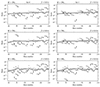 |
Fig. 2. Ratio between the final surface isotopic distributions (normalised to the abundance of 150Sm) of the Set 0 (left panel) and Set 1 (right panel) with respect to the FRUITY calculations of solar metallicity models of different masses, as indicated. |
The remaining differences between predictions from our models and FRUITY can result from: (1) Somewhat different nuclear inputs. In fact, FRUITY’s temperature and density-dependent β-decay rates of isotopes heavier than iron are based on Takahashi & Yokoi (1987) with a few exceptions (see Straniero et al. 2006, for details) and use different functions than NETGEN, and therefore Monash code to interpolate from the lowest temperature available in the database to the terrestrial values (log versus linear, respectively). (2) In our post-processing code, the equations that represent the abundance changes include nuclear burning and mixing, whereas the version of the FRANEC code that was used for the FRUITY database combines the calculation of stellar structure and nucleosynthesis, but not mixing. (3) Our method of including the 13C pocket differs from that used to produce the FRUITY results, which is based on the time-dependent convective overshoot at the base of the envelope. In addition, the 13C pocket is kept constant in our models, while it self-consistently decreases with pulse number in the FRUITY models. (4) Because of different methods and input physics, the total number of TPs differs, our models have more TPs (21, 26, and 22 vs 13, 17, and 9, for 2, 3 and 4 M⊙ models, respectively). In addition, the maximum temperatures reached by the TPs are also different: while our 2 M⊙Z = 0.014 model is cooler than the FRUITY model (280 MK versus 291 MK), 3 M⊙Z = 0.014 models reach quite similar maximum temperatures (302 MK versus 304 MK), our 4 M⊙Z = 0.014 model reaches higher maximum T (348 MK versus 312 MK) than the FRUITY stars. The effect of temperature difference is most visible at 4 M⊙, where the branching points are more active and cause a larger fluctuation in the abundances.
3.3. Comparison of Set 2 to Set 1
The extent of the difference between the predictions of Set 2 and Set 1 is affected by how much of the given isotope is produced by each model. This in turn is determined by the features of the model, the total number of neutrons available, and the differences in the nuclear input. The total amount of free neutrons is usually expressed by the time-integrated neutron flux; that is, the neutron exposure,
 (11)
(11)
The neutron exposure depends on neutron sources and the amount of Fe seed nuclei. Of the two neutron-source reactions, 13C(α, n)16O results in a higher neutron exposure than 22Ne(α, n)26Mg, because, while only a few percent of 22Ne nuclei burn, all of the 13C nuclei are completely destroyed. While the 13C abundance, and thus the number of neutrons produced, does not vary with the metallicity, the amount of Fe seeds increases with increasing metallicity. Therefore, a higher Fe abundance leads to a lower neutron exposure, as there are more Fe seeds to capture neutrons and a smaller number of free neutrons remains for the production of the s-process isotopes. The neutron exposure determines whether the neutron flux can overcome the bottlenecks at stable neutron magic nuclei (neutron number N = 28, 50, 82). Once a bottleneck is bypassed, the neutron-capture flow can reach all isotopes up to the next bottleneck, and the abundances between the bottlenecks are in roughly steady-state equilibrium (Lugaro et al. 2023b):
 (12)
(12)
The final surface normalised number abundances, Yfinali, of 34 isotopes changed by at least 10% in at least one of the Set 2 models with respect to the Set 1 models. The list of these isotopes and their YSet 2, finali/YSet 1, finali ratio are shown in Table A.3. In the following, we discuss the most relevant cases and in Table 5 we list the ratio of MACSs used in Set 2 and Set 1 for the related isotopes.
3.3.1. 64Ni
In the case of 64Ni, the ratio between its ASTRAL and KaDoNiS neutron-capture cross sections decreases with temperature (see Table 5). In general, the neutron-capture rate based on ASTRAL is the highest of the two during the 13C(α, n) phases, while the rate based on the MACS from KaDoNiS is the higher during the 22Ne(α, n) phases. In most cases, this results in a 6%–20% reduction in the abundance of 64Ni in the Set 2 models compared to the Set 1 models, except for the 4 M⊙Z = 0.007 model, where there was no difference between the predictions.
Of the five stable Ni isotopes, the most abundant 58Ni (which was used as reference isotope for the stardust grain isotopic ratio data) and 60Ni are not affected by s-process nucleosynthesis, in contrast to the much rarer 61, 62, 64Ni isotopes (1.14%, 3.63%, and 0.93% of the total Ni abundance, respectively), which can be produced by neutron captures. In Fig. 3, we compare δ60Ni58 versus δ64Ni58 from Trappitsch et al. (2018) to the predictions of the Set 0 and Set 2 models, since the final surface abundance of 64Ni also changes between Set 1 and Set 0 (see Sect. 3.1.1). We see a relatively large reduction (168–724‰, depending on the stellar model and TP) in δ64Ni58 from Set 2 to Set 0 during the stellar evolution. The Set 0 models (except for 2 M⊙Z = 0.014 model) overproduce 64Ni relative to grain data at the end of the evolution, while Set 2 models can better cover grain data. We note that the δ60Ni58 values do not change between Set 2 and Set 0. Their fluctuation in the stardust grain data is probably due to GCE as the δ60Ni58 values do not change significantly in AGB models (Trappitsch et al. 2018).
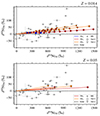 |
Fig. 3. δ60Ni58 vs δ64Ni58 from MS SiC grain data (dark grey circles with 1σ error bars from Trappitsch et al. 2018) compared to the surface evolution of Set 0 and Set 2 stellar models of solar (top panel) and of double-solar metallicity (bottom panel) of different masses (see legend). Circles (Set 0) and triangles (Set 2) on the lines represent the composition after each TDU after the envelope becomes C-rich. The dashed black lines represent the solar composition (δ = 0 by definition). |
3.3.2. 134, 135, 136, 137, 138Ba
Among the five barium isotopes on the main s-process path, the final surface abundance of 134, 136, 137Ba decreases significantly in the Set 2 models compared to the Set 1 models, consistent with the change in reaction rates (see Table 5). The only exception is the 4 M⊙Z = 0.007 model, where the final surface abundance of 137Ba slightly increases from Set 1 to Set 2, probably due to some effects related to the 137Cs branching point.
When we compare the MS SiC grain data to our predictions from the Set 1 and Set 2 models, we conclude the following: (1) The surface abundances of the s-only 136Ba used as a reference isotope (as commonly used in stardust grain analysis) are lower in Set 2 models compared to Set 1 models. Following this, the δ135Ba136 values slightly increase (by 5–11‰), except for the 4 M⊙Z = 0.03 model, where it increases more significantly (by 26‰). For the same reason, the δ134Ba136 and δ138Ba136 values also increase (by 7–38‰ and 55–110‰, respectively), despite the fact that the surface abundances of 134Ba also decrease, and the neutron-capture rate of 138Ba does not change. (2) The δ137Ba136 values decrease by 76–100‰ (and by −32‰ in 4 M⊙Z = 0.03 model) because the cross section of 137Ba increase more than the cross section of 136Ba (see Table 5). The exception is the 4 M⊙Z = 0.014 model, where 137Ba is overproduced (also relative to stardust grain data) due to activation of branching points at 134, 135, 136Cs (more details in Lugaro et al. 2018a). Vescovi & Reifarth (2021) compared the prediction of the original to the ASTRAL-based neutron-capture dataset of the FRUITY Magnetic models (Vescovi et al. 2020), and found similar results to ours in the cases of δ137Ba136 and δ138Ba136.
Comparing our predictions to the grain data, the conclusions of Lugaro et al. (2018a, based on the predictions of the Set 0 models) have not changed significantly. The two main differences are: (1) Set 2 models provide us with a better fit to the bulk of the δ137Ba136 versus δ135Ba136 stardust grain data. (2) However, the Z = 0.03 models of Set 2 produce higher δ138Ba136 than the typical values of SiC grains, which was previously only true for solar metallicity models. According to Lugaro et al. (2018a), the δ138Ba136 ratios can be reduced by decreasing the MPMZ parameter. Calculating the M = 3 M⊙ models with a lower MPMZ than the standard value (MPMZ = 5 × 10⁻⁴ M⊙ instead of 2 × 10⁻³ M⊙), the predictions of 3 M⊙Z = 0.03 model become more consistent with the grain data in both Set 1 and Set 2 (Fig. 5, bottom panel), although, as discussed in Lugaro et al. (2018a), more efficient TDU of material with such a composition is needed to reach the most extreme data points. However, the 3 M⊙Z = 0.014 model still produces higher δ138Ba136 ratios than the typical values of SiC grains (Fig. 5, top panel).
3.3.3. 186W
Due to the ASTRAL-based neutron-capture rate of 186W being lower than the JINA reaclib fit to the KaDoNiS data, the Set 2 models obtain 1.07–1.44 times more 186W than the Set 1 models at the end of the evolution. Ávila et al. (2012) reported the first tungsten isotopic measurements in SiC grains and compared the isotopic ratios to the predictions of FRUITY and the version of the Monash models3. They found that most models predict lower 186W/184W ratios than those measured in the grains. To check whether our new model predictions change this conclusion, we plot the 186W/184W versus 183W/184W predictions and data in Fig. 6. The Set 2 models provide us with higher 186W/184W ratios than the Set 1 models; in addition, the 4 M⊙Z = 0.014 model results in a similar 186W/184W ratios as the LU-41 grain. However, no models are able to match full composition of LU-41, nor the very high 186W/184W ratio shown by the bulk KJB data. It should be noted, however, that this result strongly depends on the neutron-capture rate of the branching point isotope 185W, for which no direct measurements are available, and current estimates are derived from inverse photodisintegration experiments (Sonnabend et al. 2003; Mohr et al. 2004).
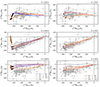 |
Fig. 4. δ134Ba136 (top row), δ137Ba136 (middle row), and δ138Ba136 (bottom row) vs δ135Ba136 from mainstream SiC grain data (dark grey circles with 1σ error bars from Savina et al. 2003; Barzyk 2007; Marhas et al. 2007; Liu et al. 2014, 2015, 2017a,b, 2019, 2022; Stephan et al. 2018, 2019) compared to the surface evolution of Set 1 and Set 2 stellar models of solar (left panels) and of double-solar metallicity (right panels) of different masses (see legend). Circles (Set 1) and triangles (Set 2) on the lines represent the composition after each TDU after the envelope becomes C-rich. The dashed black lines represent the solar composition (δ = 0 by definition). |
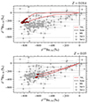 |
Fig. 5. Same as the bottom row of Fig. 4, but including only M = 3 M⊙ models calculated with MPMZ = 5 × 10⁻⁴ M⊙. |
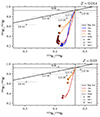 |
Fig. 6. 186W/184W vs 183W/184W from single large grains (LU) and the average of small grains (KJB, dark grey circles with 1σ error bars from Ávila et al. 2012) compared to the surface evolution of Set 1 and Set 2 stellar models of solar (top panel) and of double-solar metallicity (bottom panel) of different masses (see legend). Circles (Set 0) and triangles (Set 2) on the lines represent the composition after each TDU after the envelope becomes C-rich. The dashed black lines represent the solar composition (δ = 0 by definition). The solid black line is the regression line from Ávila et al. (2012). |
Further constrains on the s-process isotopic composition of W come from other types of meteoritic materials. From analysis of chondrules and matrix of the Allende meteorite, Budde et al. (2016) obtained a slope of +1.25 ± 0.06 (2σ) for the relationship between 182W/184W and 183W/184W (when internally normalised to 186W/184W and the solar ratios, see, e.g. Lugaro et al. 2023a, for full details), and Kruijer et al. (2014) obtained +1.41 ± 0.05 from analysis of bulk calcium-aluminium-rich inclusions (CAIs). In Fig. 7, we compare the highest and lowest observed slope, derived when considering the error bars, to the slopes derived by selected Set 2 models. The temperature conditions required to match the observations are found for stellar models in range between the 3 M⊙Z = 0.014 and the 4 M⊙Z = 0.03 models. The results do not change significantly when considering Set 1 models. Instead, they change significantly depending on the addition of the abundance of radioactive 182Hf to the abundance of 182W. In fact, the observed slopes can be matched only if 182Hf is fully included (as done in Fig. 7), otherwise all the lines have slopes between 1.8 and 2.4, much higher than observed. This indicated that Hf must have fully condensed together with W in the stardust grains that carried these anomalies into the ESS.
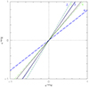 |
Fig. 7. Linear correlations between ϵ182W (including the 182Hf abundance) and ϵ183W (i.e. ratios internally normalised to 186W/184W and relative to the solar ratios, multiplied by 10 000) derived from the lowest and the upper limit of the observations (solid black lines) and from the abundances calculated at the end of the evolution of Set 2 models of Z = 0.014 (blue lines) and Z = 0.03 (green lines), with stellar mass indicated by corresponding labels and different line types: 2 M⊙ (short-dashed), 3 M⊙ (solid), and 4 M⊙ (long-dashed). We note that the M = 3 M⊙Z = 0.014 line overlaps with the line of the observational upper limit. The dotted lines indicate the solar composition. Addition of s-process material produces negative values, while removal correspond to positive values. |
Another interesting result is that when we force, for example, the 3 M⊙Z = 0.014 model to match the stardust data shown in Fig. 6, by decreasing the abundance of 183W by 0.7–0.85 and/or increasing the abundance of 186W by a factor of 2, the slope always decrease to values outside the observed range (because s-process addition produces negative values). This indicates that the stardust grains that carried the anomalies represented in Fig. 7 are not the same stardust grains plotted in Fig. 6. This may not be surprising given that the plotted single LU grains have very large size (roughly 10–20 μm), and are probably be quite rare, while the bulk grain KJB data point represents a grand average of grains of small size (∼0.5 μm). Instead, the chondrules, matrix, and CAIs data indicate a carrier with the signature of the nucleosynthesis produced in AGB models of mass and metallicity similar to those that match the composition of the single KJG grains, of typical μm size (e.g. Lugaro et al. 2018a). It is also possible that other type of grains than SiC carried the anomalies shown, as already suggested for example by Schönbächler et al. (2005), Reisberg et al. (2009) on the basis of leachates experiments.
4. Conclusions
We have studied how temperature- and density-dependent (instead of constant, terrestrial) decay rates and new neutron-capture cross sections affect s-process nucleosynthesis predictions. We have provided the first database of surface abundances and stellar yields of the isotopes heavier than iron from the Monash models. We used seven stellar structure models (Karakas 2014; Karakas & Lugaro 2016) of low-mass AGB stars, and three sets of the nuclear network (Sets 0, 1, and 2) based on three databases: JINA reaclib (Cyburt et al. 2010), NETGEN (Jorissen & Goriely 2001; Aikawa et al. 2005; Xu et al. 2013), and ASTRAL (Reifarth et al. 2018b; Vescovi & Reifarth 2021; Vescovi et al. 2023). We compared the final surface abundances of the isotopes for each set and discussed the relevant cases. We calculated the solar s-process contribution for the p-only isotopes 94Mo, 108Cd, and 152Gd, as well as for the s-only isotopes 176Lu and 176Hf, the radioactive-to-stable abundance ratios for the short-lived radionuclides 129I, 182Hf, and 205Pb, and the isolation time of the Solar System using a steady-state equation and the 205Pb/204Pb ratio. We compared our solar metallicity models with the same FRUITY (Cristallo et al. 2009, 2011, 2015) models, which also use T- and ρ-dependent decay rates. In addition to the above, we compared the predictions of the solar and double-solar metallicity models with MS presolar stardust SiC grain data for the 60Ni/64Ni, 80Kr/82Kr, 94Mo/96Mo, 134, 135, 137, 138Ba/136Ba, and 186W/184W ratios.
Our main conclusions are:
-
(1)
Taking into account the T and ρ dependence of the decay rates of the 79Se and 80Br branching isotopes (Set 1), our predictions become more consistent with the intershell 80Kr/82Kr ratios derived by Lewis et al. (1994) from stardust SiC grain data than the Set 0 models (see Table 3).
-
(2)
Taking into account the T and ρ dependence of the decay rates of the 93Zr and 94Nb branching isotopes (Set 1), the surface evolution of the 2 and 3 M⊙ solar and double-solar metallicity models follow closely the regression line of the [94Mo/96Mo] versus [92Mo/96Mo] SiC grain data (see Fig. 1). Our models quantitatively reproduce the minor s-process production of the classical p-only 94Mo observed in stardust SiC grains, of around 3–4%.
-
(3)
Taking into account the T and ρ dependence of the decay rates of the 151Sm and 152Eu branching isotopes (Set 1), we predict a high, 0.7 solar s-process contribution for the traditionally p-only 152Gd, which is consistent with results from previous studies (Arlandini et al. 1999; Bisterzo et al. 2011, 2014).
-
(4)
Our Set 1 models do not reproduce the Solar System ratio of the two s-only isotopes, 176Lu and 176Hf, due to the NETGEN rate of 176Lu incorrectly assuming thermal equilibrium between the long-lived ground state and the short-lived isomer over the whole temperature range. This problem can be solved by using a different T-dependent β-decay rate for 176Lu (e.g. from Heil et al. 2008b), but we note that the coupling between the ground state and the isomer is still uncertain and needs to be revised.
-
(5)
Taking into account the T and ρ dependence of the decay rates of 205Tl, 204Pb and 205Pb (Set 1), we cannot obtain a positive solution for the isolation time of the Solar System using the 205Pb/204Pb ratio from solar metallicity models, which suggests that the rates of the 205Tl–205Pb decay system need to be revised. This was recently done by Leckenby et al. (2024).
-
(6)
With the new (n,γ) cross sections of 64Ni and T- and ρ-dependent decay rates of 63Ni and 64Cu (Set 2 models), the δ64Ni58 values derived from the solar and double-solar metallicity models are smaller than those of Set 0, and better cover the SiC grain data (see Fig. 3).
-
(7)
With the new (n,γ) cross sections of 136, 137Ba (Set 2), the solar and double-solar metallicity models provide us with a better fit to the δ137Ba136 SiC grain data, but produce higher δ138Ba136 than the typical values of the grains and those of the previous sets (see Fig. 4).
-
(8)
The Set 2 models produce higher 186W, although they still do not match well the W isotopic composition of large SiC stardust grains well (Fig. 6). However, they do match well the W composition observed in other types of meteoritic materials (Fig. 7).
Future plans involve extending our work based on recent and future measurements of β-decay rates and (n,γ) cross sections. The PANDORA project (Plasmas for Astrophysics, Nuclear Decays Observation and Radiation for Archaeometry, Mascali et al. 2022) will be a possible source of β-decay rates from plasma measurements. The first experimental campaign involves three important isotopes for the s process: 94Nb, 134Cs, and 176Lu. The CERN neutron time-of-flight facility, n_TOF (Guerrero et al. 2013) has been providing neutron-capture cross sections for various isotopes for many years. The most recent publications present the (n,γ) cross-section measurements of 89Y (Tagliente et al. 2024), 94Nb (Balibrea-Correa et al. 2023), 140Ce (Amaducci et al. 2024), and 204Tl (Casanovas-Hoste et al. 2024) that are relevant for the s process. The effect of the 22Ne(α, n)25Mg reaction rate and its uncertainties will need to be tested. Direct cross-section measurement of this neutron-source reaction is currently being carried out at the LUNA (Laboratory for Underground Nuclear Astrophysics, Ananna et al. 2024). In addition, we plan to calculate more models with different masses and metallicities to be used as inputs for the GCE of the isotopes of the elements heavier than iron and to carry out further detailed comparisonS with meteoritic data.
Data availability
Surface isotopic abundance and stellar yield data tables of the seven stellar models of low-mass AGB stars for the three nuclear networks are available on Zenodo through the following link: https://zenodo.org/records/14981333.
Y indicates the mass fraction of helium and Z indicates the mass fraction of metals, i.e. the metallicity of the stellar model.
Regression was performed using scipy.odr (Jones et al. 2001) and the uncertainties of the data points were taken into account.
Stellar models: M = 1.25, 1.8 and 3 M⊙Z = 0.01 and M = 3 and 4 M⊙Z = 0.02.
Acknowledgments
This project has been supported by the Lendület Program LP2023-10 of the Hungarian Academy of Sciences. This work was supported by the NKFIH Excellence Grant TKP2021-NKTA-64. Amanda Karakas was supported by the Australian Research Council Centre of Excellence for All Sky Astrophysics in 3 Dimensions (ASTRO 3D), through project number CE170100013. Balázs Szányi thanks ASTRO 3D for supporting his travel to Monash University. The authors thank Marco Pignatari for his constructive comments throughout this project. The authors thank the anonymous referee for their careful comments, which helped to improve the paper.
References
- Aikawa, M., Arnould, M., Goriely, S., Jorissen, A., & Takahashi, K. 2005, A&A, 441, 1195 [NASA ADS] [CrossRef] [EDP Sciences] [Google Scholar]
- Amaducci, S., Colonna, N., Cosentino, L., et al. 2024, Phys. Rev. Lett., 132, 122701 [NASA ADS] [CrossRef] [Google Scholar]
- Amari, S., Lewis, R. S., & Anders, E. 1994, Geochim. Cosmochim. Acta, 58, 459 [Google Scholar]
- Ananna, C., Barbieri, L., Boeltzig, A., et al. 2024, Universe, 10, 228 [Google Scholar]
- Anders, E., & Grevesse, N. 1989, Geochim. Cosmochim. Acta, 53, 197 [Google Scholar]
- Arlandini, C., Käppeler, F., Wisshak, K., et al. 1999, ApJ, 525, 886 [Google Scholar]
- Asplund, M., Grevesse, N., Sauval, A. J., & Scott, P. 2009, ARA&A, 47, 481 [NASA ADS] [CrossRef] [Google Scholar]
- Ávila, J. N., Lugaro, M., Ireland, T. R., et al. 2012, ApJ, 744, 49 [Google Scholar]
- Bahcall, J. N. 1961, Phys. Rev., 124, 495 [Google Scholar]
- Balibrea-Correa, J., Babiano-Suárez, V., Lerendegui-Marco, J., et al. 2023, Eur. Phys. J. Web Conf., 279, 06004 [Google Scholar]
- Barzyk, J. G. 2007, Ph.D. Thesis, University of Chicago, USA [Google Scholar]
- Bernatowicz, T., Fraundorf, G., Ming, T., et al. 1987, Nature, 330, 728 [Google Scholar]
- Bisterzo, S., Gallino, R., Straniero, O., Cristallo, S., & Käppeler, F. 2011, MNRAS, 418, 284 [Google Scholar]
- Bisterzo, S., Travaglio, C., Gallino, R., Wiescher, M., & Käppeler, F. 2014, ApJ, 787, 10 [NASA ADS] [CrossRef] [Google Scholar]
- Bisterzo, S., Gallino, R., Käppeler, F., et al. 2015, MNRAS, 449, 506 [Google Scholar]
- Budde, G., Kleine, T., Kruijer, T. S., Burkhardt, C., & Metzler, K. 2016, Proc. Nat. Academy Sci., 113, 2886 [Google Scholar]
- Buntain, J. F., Doherty, C. L., Lugaro, M., et al. 2017, MNRAS, 471, 824 [NASA ADS] [CrossRef] [Google Scholar]
- Burbidge, E. M., Burbidge, G. R., Fowler, W. A., & Hoyle, F. 1957, Rev. Mod. Phys., 29, 547 [NASA ADS] [CrossRef] [Google Scholar]
- Busso, M., Gallino, R., & Wasserburg, G. J. 1999, ARA&A, 37, 239 [Google Scholar]
- Busso, M., Vescovi, D., Palmerini, S., Cristallo, S., & Antonuccio-Delogu, V. 2021, ApJ, 908, 55 [NASA ADS] [CrossRef] [Google Scholar]
- Cameron, A. G. W. 1957, AJ, 62, 9 [CrossRef] [Google Scholar]
- Cameron, A. G. W. 1960, AJ, 65, 485 [CrossRef] [Google Scholar]
- Cannon, R. C. 1993, MNRAS, 263, 817 [NASA ADS] [CrossRef] [Google Scholar]
- Casanovas-Hoste, A., Domingo-Pardo, C., Lerendegui-Marco, J., et al. 2024, Phys. Rev. Lett., 133, 052702 [Google Scholar]
- Caughlan, G. R., & Fowler, W. A. 1988, Atomic Data Nucl. Data Tables, 40, 283 [NASA ADS] [CrossRef] [Google Scholar]
- Côté, B., Silvia, D. W., O’Shea, B. W., Smith, B., & Wise, J. H. 2018, ApJ, 859, 67 [CrossRef] [Google Scholar]
- Côté, B., Lugaro, M., Reifarth, R., et al. 2019, ApJ, 878, 156 [CrossRef] [Google Scholar]
- Côté, B., Eichler, M., Yagüe López, A., et al. 2021, Science, 371, 945 [CrossRef] [PubMed] [Google Scholar]
- Cristallo, S., Straniero, O., Gallino, R., et al. 2009, ApJ, 696, 797 [NASA ADS] [CrossRef] [Google Scholar]
- Cristallo, S., Piersanti, L., Gallino, R., et al. 2010, J. Phys. Conf. Ser., 202, 012033 [Google Scholar]
- Cristallo, S., Piersanti, L., Straniero, O., et al. 2011, ApJS, 197, 17 [NASA ADS] [CrossRef] [Google Scholar]
- Cristallo, S., Straniero, O., Piersanti, L., & Gobrecht, D. 2015, ApJS, 219, 40 [Google Scholar]
- Cristallo, S., Nanni, A., Cescutti, G., et al. 2020, A&A, 644, A8 [CrossRef] [EDP Sciences] [Google Scholar]
- Cyburt, R. H., Amthor, A. M., Ferguson, R., et al. 2010, ApJS, 189, 240 [NASA ADS] [CrossRef] [Google Scholar]
- Dauphas, N., & Chaussidon, M. 2011, Ann. Rev. Earth Planet. Sci., 39, 351 [CrossRef] [Google Scholar]
- Davis, A. M. 2022, Ann. Rev. Nucl. Part. Sci., 72, 339 [Google Scholar]
- Dillmann, I., Heil, M., Käppeler, F., et al. 2006, in Capture Gamma-Ray Spectroscopy and Related Topics, eds. A. Woehr, & A. Aprahamian, Am. Inst. Phys. Conf. Ser., 819, 123 [NASA ADS] [CrossRef] [Google Scholar]
- Doll, C., Börner, H. G., Jaag, S., Käppeler, F., & Andrejtscheff, W. 1999, Phys. Rev. C, 59, 492 [Google Scholar]
- Fishlock, C. K., Karakas, A. I., Lugaro, M., & Yong, D. 2014, ApJ, 797, 44 [Google Scholar]
- Gallino, R. 2023, Eur. Phys. J. A, 59, 66 [Google Scholar]
- Gallino, R., Arlandini, C., Busso, M., et al. 1998, ApJ, 497, 388 [Google Scholar]
- Goriely, S. 1999, A&A, 342, 881 [NASA ADS] [Google Scholar]
- Goriely, S., & Mowlavi, N. 2000, A&A, 362, 599 [NASA ADS] [Google Scholar]
- Guerrero, C., Tsinganis, A., Berthoumieux, E., et al. 2013, Eur. Phys. J. A, 49, 27 [CrossRef] [Google Scholar]
- Heil, M., Käppeler, F., Uberseder, E., Gallino, R., & Pignatari, M. 2008a, Phys. Rev. C, 77, 015808 [CrossRef] [Google Scholar]
- Heil, M., Winckler, N., Dababneh, S., et al. 2008b, ApJ, 673, 434 [Google Scholar]
- Herwig, F. 2004, in Asymmetrical Planetary Nebulae III: Winds, Structure and the Thunderbird, eds. M. Meixner, J. H. Kastner, B. Balick, & N. Soker, ASP Conf. Ser., 313, 387 [Google Scholar]
- Hollowell, D., & Iben, I. J. 1988, ApJ, 333, L25 [Google Scholar]
- Hoppe, P., Amari, S., Zinner, E., Ireland, T., & Lewis, R. S. 1994, ApJ, 430, 870 [Google Scholar]
- Horiguchi, T., Tachibana, T., & Katakura, J. 1996, Japanese Nuclear Data Committee and Nuclear Data Center, JAERI [Google Scholar]
- Hynes, K. M., & Gyngard, F. 2009, in 40th Annual Lunar and Planetary Science Conference, Lunar and Planetary Science Conference, 1198 [Google Scholar]
- Iben, Jr., I., & Renzini, A. 1983, ARA&A, 21, 271 [NASA ADS] [CrossRef] [Google Scholar]
- Iliadis, C., Longland, R., Champagne, A. E., Coc, A., & Fitzgerald, R. 2010, Nucl. Phys. A, 841, 31 [CrossRef] [Google Scholar]
- Jones, E., Oliphant, T., Peterson, P., et al. 2001, SciPy: Open source scientific tools for Python, http://www.scipy.org/ [Google Scholar]
- Jorissen, A., & Goriely, S. 2001, Nucl. Phys. A, 688, 508 [Google Scholar]
- Käppeler, F., Gallino, R., Bisterzo, S., & Aoki, W. 2011, Rev. Mod. Phys., 83, 157 [Google Scholar]
- Karakas, A. I. 2014, MNRAS, 445, 347 [NASA ADS] [CrossRef] [Google Scholar]
- Karakas, A. I., & Lattanzio, J. C. 2014, PASA, 31 [CrossRef] [Google Scholar]
- Karakas, A. I., & Lugaro, M. 2016, ApJ, 825, 26 [NASA ADS] [CrossRef] [Google Scholar]
- Klay, N., & Käppeler, F. 1988, Phys. Rev. C, 38, 295 [CrossRef] [PubMed] [Google Scholar]
- Klay, N., Käppeler, F., Beer, H., & Schatz, G. 1991, Phys. Rev. C, 44, 2839 [Google Scholar]
- Kondev, F. G., Wang, M., Huang, W. J., Naimi, S., & Audi, G. 2021, Chin. Phys. C, 45, 030001 [NASA ADS] [CrossRef] [Google Scholar]
- Kruijer, T. S., Kleine, T., Fischer-Gödde, M., Burkhardt, C., & Wieler, R. 2014, Earth Planet. Sci. Lett., 403, 317 [CrossRef] [Google Scholar]
- Langanke, K., & Martínez-Pinedo, G. 2000, Nucl. Phys. A, 673, 481 [NASA ADS] [CrossRef] [Google Scholar]
- Lattanzio, J. C. 1986, ApJ, 311, 708 [NASA ADS] [CrossRef] [Google Scholar]
- Leckenby, G., Sidhu, R. S., Chen, R. J., et al. 2024, Nature, 635, 321 [Google Scholar]
- Lewis, R. S., Amari, S., & Anders, E. 1990, Nature, 348, 293 [CrossRef] [Google Scholar]
- Lewis, R. S., Amari, S., & Anders, E. 1994, Geochim. Cosmochim. Acta, 58, 471 [Google Scholar]
- Lewis, K. M., Lugaro, M., Gibson, B. K., & Pilkington, K. 2013, ApJ, 768, L19 [Google Scholar]
- Li, K.-A., Qi, C., Lugaro, M., et al. 2021, ApJ, 919, L19 [CrossRef] [Google Scholar]
- Liu, N., Savina, M. R., Davis, A. M., et al. 2014, ApJ, 786, 66 [NASA ADS] [CrossRef] [Google Scholar]
- Liu, N., Savina, M. R., Gallino, R., et al. 2015, ApJ, 803, 12 [NASA ADS] [CrossRef] [Google Scholar]
- Liu, N., Steele, A., Nittler, L. R., et al. 2017a, Meteor. Planet. Sci., 52, 2550 [Google Scholar]
- Liu, N., Stephan, T., Boehnke, P., et al. 2017b, ApJ, 844, L12 [NASA ADS] [CrossRef] [Google Scholar]
- Liu, N., Stephan, T., Cristallo, S., et al. 2019, ApJ, 881, 28 [CrossRef] [Google Scholar]
- Liu, N., Stephan, T., Cristallo, S., et al. 2022, Eur. Phys. J. A, 58, 216 [Google Scholar]
- Lodders, K., Palme, H., & Gail, H. P. 2009, Landolt Börnstein, 4B, 712 [Google Scholar]
- Lugaro, M., & Chieffi, A. 2018, in Astrophysics and Space Science Library, eds. R. Diehl, D. H. Hartmann, & N. Prantzos, 453, 643 [Google Scholar]
- Lugaro, M., Davis, A. M., Gallino, R., et al. 2003, ApJ, 593, 486 [NASA ADS] [CrossRef] [Google Scholar]
- Lugaro, M., Tagliente, G., Karakas, A. I., et al. 2014a, ApJ, 780, 95 [Google Scholar]
- Lugaro, M., Heger, A., Osrin, D., et al. 2014b, Science, 345, 650 [CrossRef] [PubMed] [Google Scholar]
- Lugaro, M., Karakas, A. I., Pető, M., & Plachy, E. 2018a, Geochim. Cosmochim. Acta, 221, 6 [CrossRef] [Google Scholar]
- Lugaro, M., Ott, U., & Kereszturi, Á. 2018b, Prog. Part. Nucl. Phys., 102, 1 [Google Scholar]
- Lugaro, M., Cseh, B., Világos, B., et al. 2020, ApJ, 898, 96 [NASA ADS] [CrossRef] [Google Scholar]
- Lugaro, M., Ek, M., Pető, M., et al. 2023a, Eur. Phys. J. A, 59, 53 [Google Scholar]
- Lugaro, M., Pignatari, M., Reifarth, R., & Wiescher, M. 2023b, Ann. Rev. Nucl. Part. Sci., 73, 315 [NASA ADS] [CrossRef] [Google Scholar]
- Marhas, K. K., Hoppe, P., & Ott, U. 2007, Meteor. Planet. Sci., 42, 1077 [Google Scholar]
- Mascali, D., Santonocito, D., Amaducci, S., et al. 2022, Universe, 8, 80 [CrossRef] [Google Scholar]
- Mohr, P., Shizuma, T., Ueda, H., et al. 2004, Phys. Rev. C, 69, 032801 [Google Scholar]
- Mohr, P., Bisterzo, S., Gallino, R., et al. 2009, Phys. Rev. C, 79, 045804 [Google Scholar]
- Mowlavi, N., Goriely, S., & Arnould, M. 1998, A&A, 330, 206 [NASA ADS] [Google Scholar]
- Nicolussi, G. K., Pellin, M. J., Lewis, R. S., et al. 1998, Geochim. Cosmochim. Acta, 62, 1093 [CrossRef] [Google Scholar]
- Oda, T., Hino, M., Muto, K., Takahara, M., & Sato, K. 1994, Atomic Data Nucl. Data Tables, 56, 231 [NASA ADS] [CrossRef] [Google Scholar]
- Palk, C., Andreasen, R., Rehkämper, M., et al. 2018, Meteor. Planet. Sci., 53, 167 [Google Scholar]
- Pignatari, M., & Herwig, F. 2012, Nucl. Phys. News, 22, 18 [NASA ADS] [CrossRef] [Google Scholar]
- Prantzos, N., Abia, C., Limongi, M., Chieffi, A., & Cristallo, S. 2018, MNRAS, 476, 3432 [Google Scholar]
- Prantzos, N., Abia, C., Cristallo, S., Limongi, M., & Chieffi, A. 2020, MNRAS, 491, 1832 [Google Scholar]
- Rauscher, T. 2012, ApJS, 201, 26 [NASA ADS] [CrossRef] [Google Scholar]
- Reifarth, R., Fiebiger, S., Göbel, K., et al. 2018a, Int. J. Mod. Phys. A, 33, 1843011 [Google Scholar]
- Reifarth, R., Erbacher, P., Fiebiger, S., et al. 2018b, Eur. Phys. J. Plus, 133, 424 [CrossRef] [Google Scholar]
- Reisberg, L., Dauphas, N., Luguet, A., et al. 2009, Earth Planet. Sci. Lett., 277, 334 [Google Scholar]
- Salpeter, E. E. 1955, ApJ, 121, 161 [Google Scholar]
- Savina, M. R., Pellin, M. J., Tripa, C. E., et al. 2003, Geochim. Cosmochim. Acta, 67, 3215 [Google Scholar]
- Schönbächler, M., Rehkämper, M., Fehr, M. A., et al. 2005, Geochim. Cosmochim. Acta, 69, 5113 [Google Scholar]
- Schwarzschild, M., & Härm, R. 1965, ApJ, 142, 855 [NASA ADS] [CrossRef] [Google Scholar]
- Siess, L. 2006, A&A, 448, 717 [NASA ADS] [CrossRef] [EDP Sciences] [Google Scholar]
- Sonnabend, K., Mengoni, A., Mohr, P., et al. 2003, Nucl. Phys. A, 718, 533 [Google Scholar]
- Stephan, T., Trappitsch, R., Davis, A. M., et al. 2018, Geochim. Cosmochim. Acta, 221, 109 [Google Scholar]
- Stephan, T., Trappitsch, R., Hoppe, P., et al. 2019, ApJ, 877, 101 [CrossRef] [Google Scholar]
- Stephan, T., Trappitsch, R., Hoppe, P., et al. 2024, ApJS, 270, 27 [NASA ADS] [CrossRef] [Google Scholar]
- Straniero, O., Gallino, R., Busso, M., et al. 1995, ApJ, 440, L85 [NASA ADS] [CrossRef] [Google Scholar]
- Straniero, O., Chieffi, A., Limongi, M., et al. 1997, ApJ, 478, 332 [CrossRef] [Google Scholar]
- Straniero, O., Gallino, R., & Cristallo, S. 2006, Nucl. Phys. A, 777, 311 [NASA ADS] [CrossRef] [Google Scholar]
- Tagliente, G., Milazzo, P. M., Paradela, C., et al. 2024, Eur. Phys. J. A, 60, 21 [Google Scholar]
- Takahashi, K., & Yokoi, K. 1987, Atomic Data Nucl. Data Tables, 36, 375 [NASA ADS] [CrossRef] [Google Scholar]
- Tessler, M., Zappala, J., Cristallo, S., et al. 2021, Phys. Rev. C, 104, 015806 [CrossRef] [Google Scholar]
- Thielemann, F. K., Arnould, M., & Truran, J. W. 1986, in Advances in Nuclear Astrophysics, eds. E. Vangioni-Flam, J. Audouze, M. Casse, J.-P. Chieze, & J. Tran Thanh Van, 525 [Google Scholar]
- Trappitsch, R., Stephan, T., Savina, M. R., et al. 2018, Geochim. Cosmochim. Acta, 221, 87 [Google Scholar]
- Travaglio, C., Gallino, R., Arnone, E., et al. 2004, ApJ, 601, 864 [Google Scholar]
- Travaglio, C., Röpke, F. K., Gallino, R., & Hillebrandt, W. 2011, ApJ, 739, 93 [NASA ADS] [CrossRef] [Google Scholar]
- Trueman, T. C. L., Côté, B., Yagüe López, A., et al. 2022, ApJ, 924, 10 [NASA ADS] [CrossRef] [Google Scholar]
- Truran, J. W., & Iben, I. J. r. 1977, ApJ, 216, 797 [Google Scholar]
- Van Raai, M. A., Lugaro, M., Karakas, A. I. et al. 2012, A&A, 540, A44 [NASA ADS] [CrossRef] [EDP Sciences] [Google Scholar]
- Vassiliadis, E., & Wood, P. R. 1993, ApJ, 413, 641 [Google Scholar]
- Verchovsky, A. B., Wright, I. P., & Pillinger, C. T. 2004, ApJ, 607, 611 [Google Scholar]
- Vescovi, D., & Reifarth, R. 2021, Universe, 7, 239 [Google Scholar]
- Vescovi, D., Cristallo, S., Busso, M., & Liu, N. 2020, ApJ, 897, L25 [Google Scholar]
- Vescovi, D., Reifarth, R., Lorenz, E., & Elbe, A. 2023, Eur. Phys. J. Web Conf., 279, 11011 [Google Scholar]
- Wallerstein, G., & Knapp, G. R. 1998, ARA&A, 36, 369 [NASA ADS] [CrossRef] [Google Scholar]
- Weigert, A. 1966, Z. Astrophys., 64, 395 [NASA ADS] [Google Scholar]
- Xu, Y., Goriely, S., Jorissen, A., Chen, G. L., & Arnould, M. 2013, A&A, 549, A106 [NASA ADS] [CrossRef] [EDP Sciences] [Google Scholar]
- Zinner, E. 2014, in Treatise on Geochemistry, ed. A. M. Davis (Elsevier Science), 1, 181 [Google Scholar]
Appendix A: Additional tables
YSet 1, finali/YSet 0, finali for the 30 isotopes that vary the most between the two sets.
Relevant information of each isotope case discussed in Sect. 3.1.
YSet 2, finali/YSet 1, finali for the 34 isotopes that vary the most between the two sets.
All Tables
80Kr/82Kr ratios in the selected Set 0 and Set 1 models and for each KJ fraction.
182Hf/180Hf production factors of selected Set 0 and Set 1 models, alongside the values previously used in GCE models.
YSet 1, finali/YSet 0, finali for the 30 isotopes that vary the most between the two sets.
YSet 2, finali/YSet 1, finali for the 34 isotopes that vary the most between the two sets.
All Figures
|
Fig. 1. [94Mo/96Mo] vs [92Mo/96Mo] from SiC grain data as dark grey circles MS grains and downward and upward triangles for Y and Z grains, respectively, with 1σ error bars (from Barzyk 2007; Liu et al. 2017b, 2019; Stephan et al. 2019) compared to the surface evolution of Set 0 and Set 1 stellar models of solar (left panel) and of double-solar metallicity (right panel) of different masses (see legend). Circles (Set 0) and triangles (Set 1) on the lines represent the composition after each TDU after the envelope becomes C-rich. The solid black line represents the linear regression from δ94Mo96 vs δ92Mo96, while the dashed black line represents the [94Mo/96Mo] = [92Mo/96Mo] line. |
| In the text | |
|
Fig. 2. Ratio between the final surface isotopic distributions (normalised to the abundance of 150Sm) of the Set 0 (left panel) and Set 1 (right panel) with respect to the FRUITY calculations of solar metallicity models of different masses, as indicated. |
| In the text | |
|
Fig. 3. δ60Ni58 vs δ64Ni58 from MS SiC grain data (dark grey circles with 1σ error bars from Trappitsch et al. 2018) compared to the surface evolution of Set 0 and Set 2 stellar models of solar (top panel) and of double-solar metallicity (bottom panel) of different masses (see legend). Circles (Set 0) and triangles (Set 2) on the lines represent the composition after each TDU after the envelope becomes C-rich. The dashed black lines represent the solar composition (δ = 0 by definition). |
| In the text | |
|
Fig. 4. δ134Ba136 (top row), δ137Ba136 (middle row), and δ138Ba136 (bottom row) vs δ135Ba136 from mainstream SiC grain data (dark grey circles with 1σ error bars from Savina et al. 2003; Barzyk 2007; Marhas et al. 2007; Liu et al. 2014, 2015, 2017a,b, 2019, 2022; Stephan et al. 2018, 2019) compared to the surface evolution of Set 1 and Set 2 stellar models of solar (left panels) and of double-solar metallicity (right panels) of different masses (see legend). Circles (Set 1) and triangles (Set 2) on the lines represent the composition after each TDU after the envelope becomes C-rich. The dashed black lines represent the solar composition (δ = 0 by definition). |
| In the text | |
|
Fig. 5. Same as the bottom row of Fig. 4, but including only M = 3 M⊙ models calculated with MPMZ = 5 × 10⁻⁴ M⊙. |
| In the text | |
|
Fig. 6. 186W/184W vs 183W/184W from single large grains (LU) and the average of small grains (KJB, dark grey circles with 1σ error bars from Ávila et al. 2012) compared to the surface evolution of Set 1 and Set 2 stellar models of solar (top panel) and of double-solar metallicity (bottom panel) of different masses (see legend). Circles (Set 0) and triangles (Set 2) on the lines represent the composition after each TDU after the envelope becomes C-rich. The dashed black lines represent the solar composition (δ = 0 by definition). The solid black line is the regression line from Ávila et al. (2012). |
| In the text | |
|
Fig. 7. Linear correlations between ϵ182W (including the 182Hf abundance) and ϵ183W (i.e. ratios internally normalised to 186W/184W and relative to the solar ratios, multiplied by 10 000) derived from the lowest and the upper limit of the observations (solid black lines) and from the abundances calculated at the end of the evolution of Set 2 models of Z = 0.014 (blue lines) and Z = 0.03 (green lines), with stellar mass indicated by corresponding labels and different line types: 2 M⊙ (short-dashed), 3 M⊙ (solid), and 4 M⊙ (long-dashed). We note that the M = 3 M⊙Z = 0.014 line overlaps with the line of the observational upper limit. The dotted lines indicate the solar composition. Addition of s-process material produces negative values, while removal correspond to positive values. |
| In the text | |
Current usage metrics show cumulative count of Article Views (full-text article views including HTML views, PDF and ePub downloads, according to the available data) and Abstracts Views on Vision4Press platform.
Data correspond to usage on the plateform after 2015. The current usage metrics is available 48-96 hours after online publication and is updated daily on week days.
Initial download of the metrics may take a while.