| Issue |
A&A
Volume 656, December 2021
|
|
|---|---|---|
| Article Number | A67 | |
| Number of page(s) | 11 | |
| Section | Stellar atmospheres | |
| DOI | https://doi.org/10.1051/0004-6361/202142056 | |
| Published online | 03 December 2021 | |
Abundance of barium in the atmospheres of red giants in the Galactic globular cluster NGC 104 (47 Tuc)★,★★
1
Institute of Theoretical Physics and Astronomy, Vilnius University,
Saulėtekio al. 3,
Vilnius
10257, Lithuania
e-mail: This email address is being protected from spambots. You need JavaScript enabled to view it.
2
Crimean Astrophysical Observatory,
Nauchny
298409,
Crimea
Received:
19
August
2021
Accepted:
6
September
2021
Abstract
Context. While most (if not all) Type I Galactic globular clusters (GGCs) are characterised by spreads in the abundances of light chemical elements (e.g. Li, N, O, Na, Mg, Al), it is not yet well established whether similar spreads may exist in s-process elements as well.
Aims. We investigated the possible difference in Ba abundance between the primordial (1P) and polluted (2P) stars in the Galactic globular cluster (GGC) 47 Tuc (NGC 104). For this purpose, we obtained homogeneous abundances of Fe, Na, and Ba in a sample of 261 red giant branch (RGB) stars, which comprises the largest sample used for Na and Ba abundance analysis in any GGC so far.
Methods. Abundances of Na and Ba were determined using archival GIRAFFE/VLT spectra and 1D non-local thermodynamic equilibrium (NLTE) abundance analysis methodology.
Results. Contrary to the finding of Gratton et al. (2013, A&A, 549, A41), we did not detect any significant Ba–Na correlation or 2P–1P Ba abundance difference in the sample of 261 RGB stars in 47 Tuc. This corroborates the result of D’Orazi et al. (2010, ApJ, 719, L213), who found no statistically significant Ba–Na correlation in 110 RGB stars in this GGC. The average barium-to-iron ratio obtained in the sample of 261 RGB stars, ⟨[Ba/Fe]1D NLTE⟩ = −0.01 ± 0.06, agrees well with those determined in Galactic field stars at this metallicity and may therefore represent the abundance of primordial proto-cluster gas that has not been altered during the subsequent chemical evolution of the cluster.
Key words: techniques: spectroscopic / stars: abundances / stars: late-type / globular clusters: individual: NGC 104
Full Table D.1 is only available at the CDS via anonymous ftp to cdsarc.u-strasbg.fr (130.79.128.5) or via http://cdsarc.u-strasbg.fr/viz-bin/cat/J/A+A/656/A67
Based on observations obtained at the European Southern Observatory (ESO) Very Large Telescope (VLT) at Paranal Observatory, Chile.
© ESO 2021
1 Introduction
Most, if not all, Galactic globular clusters contain multiple stellar populations that are characterised by different abundances of chemical elements, radial distributions in the given GGC, and kinematic properties (see e.g. Bastian & Lardo 2018, for a review). It is typically assumed that a fraction of the GGC stars, that is, the so-called second-generation stars (2P), were enriched in certain chemical elements and depleted in others by some first-generation (1P) polluters. A number of enrichment scenarios have been proposed to explain the observed properties of the GGCs by involving various potential polluters, such as fast-rotating massive stars (FRMS; e.g. Decressin et al. 2007), asymptotic giant branch (AGB) stars (e.g. D’Antona et al. 2016), supermassive stars (SMS, ~104 M⊙; e.g. Denisenkov & Hartwick 2014; Gieles et al. 2018). Unfortunately, none of the proposed scenarios is capable of simultaneously explaining chemical and kinematic differences between the 1P and 2P stars (Bastian & Lardo 2018; Gratton et al. 2019).
The 1P–2P differences in the abundances of chemical elements have been detected as correlations or anti-correlations between the abundances of light elements: the Na–Li (Bonifacio et al. 2007) correlation, along with the O–Na, Mg–Al (Carretta et al. 2009), and Li–O (Pasquini et al. 2005; Shen et al. 2010) anti-correlations. Except for the so-called Type II GGCs (see Marino et al. 2015, 2019 for details), the majority of Galactic GGCs (Type I) seem to be uniform in their Fe-group, as well as s- and r-process element abundances.
As for the s-process elements, results of several studies have suggested that there may be some variation in their abundances in several Type I GGCs, too. For example, Gratton et al. (2013) reported a possible Na–Ba correlation in the sample of 106 red horizontal branch (RHB) stars in NGC 104 (47 Tuc). While the statistical significance of the possible correlation was found to be high, the authors have warned thatbecause of a small range in the [Ba/Fe] variation and [Na/O] correlation with the effective temperature along the horizontal branch (HB), their result needed to be confirmed in further studies before claiming a definitive detection (Gratton et al. 2013). Some other studies have shown tentative signs for a possible correlation between the abundances of light and s-process elements in other Type I GGCs, such as signatures for Sr–Na and Y–Na relations in M 4 (Spite et al. 2016; Villanova & Geisler 2011; but see also D’Orazi et al. 2013). In addition, our recent analysis of Zr abundance in 237 RGB stars in 47 Tuc suggests theexistence of weak but statistically significant Na–Zr correlation and 2P–1P Zr abundance difference of Δ[Zr/Fe]2P−1P ≈ 0.06 (Kolomiecas et al. 2021). The existence of such correlations would indicate that the light and s-process elements should have been produced in the same polluters that have enriched the 2P stars in some elements and depleted in others. Unfortunately, the data obtained so far is inconclusive thus further analysis of more s-process elements in the larger samples of GGC stars would be desirable.
With an aim of shedding more light on the possible 1P–2P differences in s-process element abundances, in this study, we determined Ba abundances in 261 RGB stars in 47 Tuc, a Type I GGC (Marino et al. 2019). To the best of our knowledge, this is the only GGC for which a tentative detection of statistically significant relation between the light and s-process element abundances has been reported. Therefore, our primary goal was to verify whether the Na–Ba correlation or 1P–2P Ba abundance difference could be detected in our RGB star sample, which is the largest one for which Ba abundance was determined in any GGC thus far.
The paper is structured as follows. Following a short introduction, we provide a brief description of the observational data in Sect. 2 and our abundance determination methodology in Sect. 4. The obtained results are discussed in Sect. 5 and the main findings are summarised in Sect. 6.
Spectroscopic data used in this work.
2 Observational data
In this work, we studied a sample of RGB stars using the high-resolution spectra that were obtained with GIRAFFE/VLT during three observing programs: 072.D-0777(A), PI: François; 073.D-0211(A), PI: Carretta; and 088.D-0026(A), PI: McDonald (Table 1). Individual spectra were retrieved for the analysis from the ESO Advanced Data Products Archive1. Our stellar sample overlaps with that utilised by Kolomiecas et al. (2021) in their study of Zr in 47 Tuc (228 stars in common), but it also includes 33 additional targets that were not analysed in Kolomiecas et al. (2021).
Median-averaged sky spectrum was obtained from the dedicated sky fibres and subsequently was subtracted from the individual spectra of all target stars. In the case of the program 088.D-0026(A) where three exposures for the same targets were available, spectra were co-added to increase signal-to-noise ratio (S/N), with the latter determined at the continuum level in the vicinity of the investigated Na I and Ba II lines (~ 619.7 nm). The S/N of the final spectra varied from S∕N ~ 220 for the targets at Teff ~ 4200 K to S∕N ~ 60 at Teff ~ 4700 K. All target spectra were continuum-normalised using the splot task under IRAF (Tody 1986). Radial velocities were determined using the fxcor task in IRAF and cross-correlation technique. For this, we used synthetic spectrum computed with the model atmosphere having Teff = 4500 K, log g = 1.90, and ![Mathematical equation: ${\left[\mathrm{Fe}/\mathrm{H}\right]}\,{=}\,{-}0.7$](/articles/aa/full_html/2021/12/aa42056-21/aa42056-21-eq2.png) to represent a typical RGB star in 47 Tuc. The obtained radial velocities were then used to shift the wavelengths to the rest frame with the dopcor task in IRAF.
to represent a typical RGB star in 47 Tuc. The obtained radial velocities were then used to shift the wavelengths to the rest frame with the dopcor task in IRAF.
Only RGB stars were selected for the abundance analysis, by discarding HB and AGB stars based on their position in the V − (V − I) colour magnitude diagram. Before performing the abundance analysis, we verified that all targets are members of 47 Tuc based on their proper motions taken from the Gaia EDR3 catalogue (Gaia Collaboration 2021). Following Milone et al. (2018), we required that the proper motions of the cluster member stars did not deviate by more than 1.5 mas yr−1 from the mean cluster proper motion, μRA = 5.25 mas yr−1 and μDec = −2.53 mas yr−1 (Baumgardt et al. 2019).
Stars common to several programs were identified by cross-matching their coordinates within the 1 arcsec radius. This resulted in 14 stars in common to the 073.D-0211(A) and 088.D-0026(A) samples, 23 stars to 072.D-0777(A) and 088.D-0026(A), 17 stars to 072.D-0777(A) and 073.D-0211(A), and 5 stars in common to all three samples (Table A.1). Abundances of these stars were computed by averaging those obtained using spectra of individual observing programs.
The final target sample consisted of 261 unique RGB stars for which we determined Fe, Na, and Ba abundances. Our RGB sample is therefore somewhat larger than that of Kolomiecas et al. (2021, 237 objects) because it includes stars with Teff > 4800 K that were discarded from their analysis.
3 Atmospheric parameters
Atmospheric parameters for the majority of targets (228 stars) were determined by Kolomiecas et al. (2021). For the remaining 33 stars, we used the same procedure as utilised by the latter authors. With this approach, effective temperatures were determined using photometry from Bergbusch & Stetson (2009) and color-Teff calibration of Ramirez & Melendez (2005). The obtained values were verified by checking trends in the iron abundance-lower excitation potential plane. In most cases, the slopes were consistent with zero, thereby suggesting a good agreement between the photometric and spectroscopic Teff values.
Surface gravities were obtained by using a classical relation between stellar mass, luminosity, effective temperature, and surface gravity. This decision was made because only a few Fe II lines were available in the stellar spectra (typically between one and four lines). To compute gravities from photometry, we assumed an identical mass of 0.87 M⊙ for all RGB stars investigated in this work, as indicated by the Yonsei-Yale isochrone of 12 Gyr and ![Mathematical equation: ${\left[\mathrm{M}/\mathrm{H}\right]}\,{=}\,{-}0.68$](/articles/aa/full_html/2021/12/aa42056-21/aa42056-21-eq3.png) (Kim et al. 2002). Bolometric luminosities were computed using relation between the bolometric correction, Teff, and metallicity from Alonso et al. (1999).
(Kim et al. 2002). Bolometric luminosities were computed using relation between the bolometric correction, Teff, and metallicity from Alonso et al. (1999).
Microturbulence velocities were obtained by enforcing zero trend in the iron abundance-equivalent width plane while keeping photometric effective temperature fixed. In this procedure, strong lines were neglected (W > 15 pm) because of their reduced sensitivity to microturbulence velocity. Due to small number (17–28) of iron lines, the estimated accuracy of microturbulence velocity was ≈ 0.2 km s−1 and represents the main source of uncertainty in the determined Ba abundances (Sect. 4.5). The location of the target RGB stars in the Teff − logg plane is shown in Fig. 1. The atmospheric parameters of the individual target stars are listed in Table D.1.
Atomic parameters of Na I and Ba II lines used in this study.
 |
Fig. 1 Target RGB stars in the Teff − logg
plane. The red line is Yonsei-Yale (Kim et al. 2002) isochrone (12 Gyr, |
![Mathematical equation: ${\left[\mathrm{M}/\mathrm{H}\right]}\,{=}\,{-}0.68$](/articles/aa/full_html/2021/12/aa42056-21/aa42056-21-eq25.png)
4 Abundance analysis
Because the stellar sample used in the present study overlaps with the one investigated by Kolomiecas et al. (2021), abundances of Fe and Na in targets common to the two studies (228 stars) were taken from Kolomiecas et al. (2021). In addition, we determined Fe and Na abundances in 33 RGB stars and Ba abundances in 261 stars. In both studies, an abundance analysis of Fe and Na was performed following strictly identical procedures. Abundances of Na and Ba were determined using ATLAS9 model atmospheres (Kurucz 1993; Sbordone et al. 2004; Sbordone 2005) and spectral synthesis, under the assumption of non-local thermodynamic equilibrium (NLTE); local thermodynamic equilibrium (LTE) was assumed in the analysis of Fe. Procedures involved in the abundance determination are described below.
4.1 Reference abundances in the Sun
Reference abundances in the Sun were determined using the Kitt Peak Solar Flux atlas (Kurucz et al. 1984). To briefly summarise, Fe abundance was obtained using the equivalent width method, with the latter determined by fitting the Voigt profiles to the observed spectral line profiles. The Fe I and Fe II line list used for abundance determination is provided in Table B.1. Oscillator strength data were obtained from the VALD3 database (Ryabchikova et al. 2015).
The microturbulence velocity was obtained by iteration until there was a zero trend of iron abundance with the line strength. Our determined value of ξmicro = 0.93 km s−1 is in good agreement with the typical value of 0.9–1.0 km s−1 cited in the literature (Doyle et al. 2014). The average solar iron abundance obtained with the determined microturbulence velocity was A(Fe) = 7.55 ± 0.01 (σ = 0.06; here, ± 0.01 is the error of the mean, σ denotes standard deviation due to the line-to-line abundance variation), which was obtained from 29 lines with W < 10.5 pm (Table B.1). Although the scatter is significant, the average abundance is in good agreement with those available in the literature, for instance, A(Fe) = 7.51 ± 0.06 from Caffau et al. (2011).
For the solar Na abundances, we used A(Na) = 6.17, which was determined with the NLTE spectral line synthesis methodology (Sect. 4.3) and by using the same Na I lines, as utilised in the analysis of the target stars in 47 Tuc. This value agrees well with those obtained in the earlier studies, for instance, 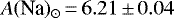 derived by Scott et al. (2015).
Solar abundance of Ba was obtained by utilising the NLTE methodology (Sect. 4.4). The determined value, A(Ba) = 2.17, agrees reasonably well with 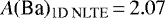 and
and 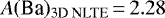 derived by Gallagher et al. (2020) and coincides with the meteoritic value of 2.17 ± 0.02 from Lodders (2021).
4.2 Determination of Fe abundance
Abundancesof Fe in the target RGB stars were obtained using a set of 17–28 Fe I lines (612.79−691.67 nm), with the line lower level excitation potentials in the range of 2.18–4.61 eV (Table B.1). The mean value obtained in the sample of 261 stars was ⟨[Fe/H]⟩ = −0.75 ± 0.05 (the error denotes the standard deviation due to the star-to-star abundance scatter), which agrees well with the values determined in the earlier studies (cf. ⟨[Fe/H]⟩ = −0.74 ± 0.05, Carretta et al. 2009, 114 RGB stars). The Fe abundances obtained in 261 target RGB stars are listed in Table D.1.
4.3 Determination of Na abundance
Two Na I lines located at 615.42 nm and 616.07 nm were used in the determination of Na abundances (Table 2). The model atom of Na used in this work was the same as described in Dobrovolskas et al. (2014). It consisted of the first 20 energy levels of Na I and the ground level of Na II, with a total of 46 radiative transitions taken into account. The rate coefficients of collisions with hydrogen atoms for the lower nine levels of Na I were taken from Barklem et al. (2010). Examples of the best-fitted Na I line profiles in the Na-poor and Na-rich stars are shown in Fig. 2, while the Na abundances determined in all target stars are plotted in the middle row of Fig. 3 and are listed in Table D.1. The Na NLTE–LTE abundance corrections,  , were in the range − 0.07...−0.27, depending on the strength of the spectral line and effective temperature of the target star (Table 3).
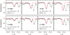 |
Fig. 2 Examples of the observed (black dots) and best-fitted synthetic Na I line profiles (red lines) in the GIRAFFE spectra of the target stars characterised by different Na abundances and effective temperatures (Teff ≈ 4250 K, top row; Teff ≈ 4750 K, bottom row). The continuum level is shown as the gray dashed line. |
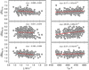 |
Fig. 3 Fe (top row), Na (middle row), and Ba (bottom row) abundances plotted against the microturbulence velocity (left column) and effective temperature (right column). In all panels, the linear fits to the data are shown as the solid red lines. |
1DNLTE-LTE abundance corrections for Na and Ba.
4.4 Determination of Ba abundance
As in the case of Na, abundances of Ba were determined using spectral synthesis approach, under the assumption of NLTE. Two Ba II lines located at 614.17 and 649.69 nm were used for the analysis whenever possible though in most cases only the 614.17 nm line was available for the analysis (Table 2). The level departure coefficients and spectral lineprofiles were computed using the version of the MULTI code (Carlsson 1986) modified by (Korotin et al. 1999). To take into account the fact that 614.17 nm line is blended with Fe I line, the spectra were computed with the SynthV code (Tsymbal 1996). For this, we used NLTE departure coefficients of Ba computed with the MULTI code while the Fe I line was synthesised under the assumption of LTE. The model atom of Ba used in this work was the same as described in Andrievsky et al. (2009). It consisted of 31 levels of Ba I, 101 levels of Ba II (n < 50), and the ground level of Ba III. In total, 91 bound-bound transitions between the lowest 28 energy levels (n < 12, l < 5) of Ba II were taken into account. Fine structure was included for the levels 5d2 D and 6p2P0, according tothe prescription given in Andrievsky et al. (2009). Following the latter study, the hyperfine structure of the 649.69 nm line was approximated using three components (lines).
Only the 088.D-0026(A) sample contained spectra where both Ba II lines were available for every target star. In this case, the final Ba abundance value was taken as an average of estimates obtained from the two lines. In all other cases Ba abundance was determined using a single 614.17 nm line. Since Ba II lines are strong, we did not take into account their possible contamination by CN lines and their influence on the Ba abundance determination. We nevertheless estimate that this effect should not exceed 0.01 dex. The obtained Ba abundances are shown in the bottom row of Fig. 3 and are listed in Table D.1. Typical examples of the 1D NLTE synthetic spectrum fits to the Ba II 614.17 nm spectral line in the target stars characterised by different effective temperatures are provided in Fig. 4. The Δ1D NLTE-LTE abundance corrections for Ba were in the range − 0.06...−0.10, increasing in magnitude at higher effective temperatures (Table 3).
The average barium-to-iron abundance ratio determined in the sample of 261 was  where the error is standard deviation due to star-to-star abundance variation.
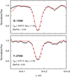 |
Fig. 4 Examples of the observed (black dots) and best-fitted synthetic spectra in the vicinity of the 614.17 nm Ba II line (red lines) in the GIRAFFE spectra of the target stars characterised by different effective temperatures (Teff ≈ 4250 K, top panel; Teff ≈ 4750 K, bottom panel). The continuum level is shown as the gray dashed line. |
4.5 Errors in the determined Fe, Na, and Ba abundances
Uncertainties in the determined Fe, Na, and Ba abundances were determined using the prescription given in Černiauskas et al. (2018), by utilising ATLAS9 models computed with Teff = 4250 K, log g = 1.35; and Teff = 4750 K, log g = 2.40. In essence, we first estimated errors in the effective temperature, surface gravity, microturbulence velocity, continuum determination, and line profile fitting. For all sample stars, we assumed identical uncertainties in the effective temperature, surface gravity, and microturbulence velocity, which were 80 K, 0.1 dex, and 0.1 km s−1, respectively.Error of the continuum placement was determined by computing standard deviation of the continuum, σcont, in the vicinity of the investigated spectral lines and then changing continuum level by ± 1σcont from the adopted level and re-determining abundances. The fit error was estimated by computing standard deviation of the difference between the observed and best-fitted spectral line profiles. Again, the synthetic spectrum was changed by ± 1σ and the resulting difference in the abundance was computed. These individual errors were then added in quadratures and were used further as uncertainties in the determined abundances of Fe, Na, and Ba. The typical abundance errors are provided in Table 4.
Typical Fe, Na, and Ba abundance measurement errors.
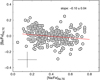 |
Fig. 5 [Ba/Fe] abundance ratios determined in 261 RGB stars in 47 Tuc, plotted versus their [Na/Fe] abundance rations. Typical abundance error bars are shown in the bottom left corner. The linear fit to the data is shown as the solid red line. |
5 Results and discussion
5.1 Possible Ba–Na anti-correlation in the RGB stars in 47 Tuc?
The barium-to-iron abundance ratios, ![Mathematical equation: ${\left[\mathrm{Ba}/\mathrm{Fe}\right]}$](/articles/aa/full_html/2021/12/aa42056-21/aa42056-21-eq9.png) , determined in 261 RGB stars show a weak but statistically significant anti-correlation with the sodium-to-iron abundance ratios,
, determined in 261 RGB stars show a weak but statistically significant anti-correlation with the sodium-to-iron abundance ratios, ![Mathematical equation: ${\left[\mathrm{Na}/\mathrm{Fe}\right]}{}$](/articles/aa/full_html/2021/12/aa42056-21/aa42056-21-eq10.png) (Fig. 5), with Pearson’s correlation coefficient, rP = −0.18. Assuming a null-hypothesis that there is no correlation between the two abundance ratios, the Student’s t-test gives a probability of pP = 2.9 × 10⁻³ that such rP value could be obtained by chance (Table 5). The Spearman’s rank correlation coefficient and the p-value are, respectively,ρS = − 0.20 and pS = 1.3 × 10⁻³, while for the Kendall’s rank correlation, the two values are τK = − 0.14 and pK = 6.9 × 10⁻⁴, respectively.
(Fig. 5), with Pearson’s correlation coefficient, rP = −0.18. Assuming a null-hypothesis that there is no correlation between the two abundance ratios, the Student’s t-test gives a probability of pP = 2.9 × 10⁻³ that such rP value could be obtained by chance (Table 5). The Spearman’s rank correlation coefficient and the p-value are, respectively,ρS = − 0.20 and pS = 1.3 × 10⁻³, while for the Kendall’s rank correlation, the two values are τK = − 0.14 and pK = 6.9 × 10⁻⁴, respectively.
We also checked whether such an anti-correlation could exist between the determined [Ba/Fe] abundance ratios and the distance of the target RGB stars from the cluster center. For this, we adopted the coordinates of the 47 Tuc center, α0 (J2000) = 6.023625 deg and δ0 (J2000) = −72.081276 deg, from Baumgardt et al. (2019) and the half-mass radius of rh = 174 arcsec from Trager et al. (1993). Our data suggest a weak correlation in the [Ba/Fe] − rh plane, with rP = 0.14 and pP = 0.019 (Fig. 6); similar values were obtained for the Spearman’s and Kendall’s rank correlation coefficients.
On the one hand, these results may suggest that in 47 Tuc the 1P stars (lower Na abundances) are more abundant in Ba than the 2P stars(higher Na abundances; Fig. 5). Because the 2P stars tend to concentrate towards the cluster center in this and other GGCs (e.g. Kučinskas et al. 2014), this is expected to lead to a weak correlation in the [Ba/Fe] − rh plane. This is exactly what our data suggest (Fig. 6). However, this result would be difficult to explain from the nucleosynthesis point of view. It is well known that Ba could be synthesised either in the low- and intermediate-mass AGB stars via the main s-process or during the central He-burning phase in the massive rotating stars. However, the trends suggested by our data would require a mechanism which would destroy Ba in the 2P stars instead of synthesising it like, for instance, Na.
On the other hand, no Ba–Na anti-correlation is seen in the absolute abundance plane, A(Ba) − A(Na) (Fig. 7). In this case, we obtained rP = 0.04 and pP = 0.52, with similarresults also for the Spearman’s and Kendall’s rank correlation coefficients: ρS = 0.03 and pS = 0.63 for the former, and τK = 0.03 and pK = 0.53 for the latter. No trend was detected in the [Ba/Fe] − rh plane either, with rP = − 0.002 ± 0.006 and pP = 0.984. This would therefore suggest that the anti-correlation in the [Ba/Fe] −[Na/Fe] plane and correlation in the [Ba/Fe] − rh plane may be caused by the variation in Fe abundance alone.
A closer inspection of the data has shown that the Ba-Na anti-correlation in the ![Mathematical equation: ${\left[\mathrm{Ba}/\mathrm{Fe}\right]}-{\left[\mathrm{Na}/\mathrm{Fe}\right]}$](/articles/aa/full_html/2021/12/aa42056-21/aa42056-21-eq11.png) plane has been detectable only in a single effective temperature interval (bin), 4600 ≤ Teff < 4700 K, with a possible weaker trend seen also in the 4400 ≤ Teff < 4500 K bin (Table 5). No statistically significant correlation was detected in other Δ = 100 K wide effective temperature bins. It therefore seems that the anti-correlation in the 4600 ≤ Teff < 4700 K bin was caused by several outlying stars with the somewhat higher and lower Ba abundances at the lowest and highest Na abundance ends, respectively (see Appendix C). No residual correlation is seen if these outliers are excluded.
plane has been detectable only in a single effective temperature interval (bin), 4600 ≤ Teff < 4700 K, with a possible weaker trend seen also in the 4400 ≤ Teff < 4500 K bin (Table 5). No statistically significant correlation was detected in other Δ = 100 K wide effective temperature bins. It therefore seems that the anti-correlation in the 4600 ≤ Teff < 4700 K bin was caused by several outlying stars with the somewhat higher and lower Ba abundances at the lowest and highest Na abundance ends, respectively (see Appendix C). No residual correlation is seen if these outliers are excluded.
It is also important to stress that abundances of all three elements analysed in this study show trends with the microturbulence velocity (Fig. 3). The most likely explanation for this is that microturbulence velocities were slightly underestimated in the hotter (Teff ≿ 4700 K) stars which are fainter and therefore their spectra are of lower quality. For these stars, a slight overestimate of the continuum during the determination of microturbulence velocities would lead to a systematically larger abundances determined from the weaker Fe I lines with respect to those obtained from the stronger lines. This, in turn, would require a lower microturbulence velocity value to eliminate the trend of iron abundance with the equivalent width. Because the Ba II lines are the strongest of all three elements studied, it is not surprising that there is the strongest trend of abundance versus microturbulence velocity for barium. Thus, overestimated Ba abundances in stars with the lowest microturbulence velocities (i.e. those with the highest effective temperatures) could also contribute to the spurious ![Mathematical equation: ${\left[\mathrm{Ba}/\mathrm{Fe}\right]}-{\left[\mathrm{Na}/\mathrm{Fe}\right]}$](/articles/aa/full_html/2021/12/aa42056-21/aa42056-21-eq12.png) anti-correlation.
anti-correlation.
Therefore, the most likely reason for the anti-correlation seen in the ![Mathematical equation: ${\left[\mathrm{Ba}/\mathrm{Fe}\right]}-{\left[\mathrm{Na}/\mathrm{Fe}\right]}$](/articles/aa/full_html/2021/12/aa42056-21/aa42056-21-eq13.png) plane and correlation in the
plane and correlation in the ![Mathematical equation: ${\left[\mathrm{Ba}/\mathrm{Fe}\right]}-r_{\mathrm h}$](/articles/aa/full_html/2021/12/aa42056-21/aa42056-21-eq14.png) plane may be a random fluctuation in Ba abundances in several stars with the extreme Na abundances in the 4600 ≤ Teff < 4700 K effective temperature bin. This deviation in a single Teff bin can not be explained by e.g. the lower quality of the spectra, because for the hotter and therefore fainter stars there is no such correlation. Similarly, there is no plausible astrophysical reason why such correlation should exist in a single Teff bin only. We also note that no Ba–Na correlation was detected by D’Orazi et al. (2010) in their analysis of 110 RGB stars in 47 Tuc, which indirectly supports our assertion that the
plane may be a random fluctuation in Ba abundances in several stars with the extreme Na abundances in the 4600 ≤ Teff < 4700 K effective temperature bin. This deviation in a single Teff bin can not be explained by e.g. the lower quality of the spectra, because for the hotter and therefore fainter stars there is no such correlation. Similarly, there is no plausible astrophysical reason why such correlation should exist in a single Teff bin only. We also note that no Ba–Na correlation was detected by D’Orazi et al. (2010) in their analysis of 110 RGB stars in 47 Tuc, which indirectly supports our assertion that the ![Mathematical equation: ${\left[\mathrm{Ba}/\mathrm{Fe}\right]}-{\left[\mathrm{Na}/\mathrm{Fe}\right]}$](/articles/aa/full_html/2021/12/aa42056-21/aa42056-21-eq15.png) anti-correlation detected in our study is, in fact, spurious. This said, it would be nevertheless interesting to see whether the Ba–Na – or any correlation between any other s-process and light elements – could be seen in other GGCs, especially given the tentative detection of Zr–Na correlation in the RGB stars of 47 Tuc that is suggested in the analysis of Kolomiecas et al. (2021).
anti-correlation detected in our study is, in fact, spurious. This said, it would be nevertheless interesting to see whether the Ba–Na – or any correlation between any other s-process and light elements – could be seen in other GGCs, especially given the tentative detection of Zr–Na correlation in the RGB stars of 47 Tuc that is suggested in the analysis of Kolomiecas et al. (2021).
[Ba/Fe]−[Na/Fe] abundance correlation coefficients and their in the full sample of 261 RGB stars in 47 Tuc and sub-samples divided into ΔTeff = 100 K-wide bins.
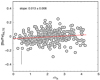 |
Fig. 6 [Ba/Fe] abundance ratios obtained in 261 RGB stars in 47 Tuc, plotted versus relative radial distance from the cluster center. Cluster half-mass radius, rh = 174 arcsec, was taken from Trager et al. (1993). Linear fit to the data is marked as the solid red line. Typical abundance error is shown as the vertical bar in the bottom left corner. |
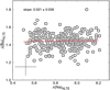 |
Fig. 7 Absolute abundances of Ba and Na in the A(Ba) − A(Na) plane. Typical abundance error bars are shown in the bottom left corner. The linear fit to the data is shown as the solid red line. |
5.2 Average Ba abundance in the RGB stars in 47 Tuc
Until now, Ba abundance in 47 Tuc has been determined by a number of studies. In one of the earlier attempts, James et al. (2004) investigated Ba in the atmospheres of turn-off (TO) and subgiant (SGB) stars in 47 Tuc. The average Ba LTE abundance determined in eight SGB stars was ![Mathematical equation: ${\left[\mathrm{Ba}/\mathrm{Fe}\right]}$](/articles/aa/full_html/2021/12/aa42056-21/aa42056-21-eq16.png) = +0.35, with an only slightly lower value of
= +0.35, with an only slightly lower value of ![Mathematical equation: ${\left[\mathrm{Ba}/\mathrm{Fe}\right]}$](/articles/aa/full_html/2021/12/aa42056-21/aa42056-21-eq17.png) = +0.22 obtained in three TO stars. The average value derived for these stars is, therefore, slightly larger than the average abundance obtained in our study, given that we determined
= +0.22 obtained in three TO stars. The average value derived for these stars is, therefore, slightly larger than the average abundance obtained in our study, given that we determined  and that the mean 1D NLTE–LTE Ba abundance correction is approximately − 0.10 dex.
One of the most comprehensive Ba abundance studies in the GGCs was performed by D’Orazi et al. (2010), who studied 1200 stars in 15 GGCs. In case of 47 Tuc, they obtained a mean value of  in the sample of 110 RGB stars (the error is standard deviation due to star-to-star abundance variation). Again, this value agrees well with that obtained in the present study if the NLTE–LTE correction (approximately − 0.10 dex) is taken into account. Similarly, a reasonable agreement is obtained with the average Ba LTE abundances obtained by Worley et al. (2010,
 ![Mathematical equation: ${\left[\mathrm{Ba}/\mathrm{Fe}\right]}\,{=}\,0.34\,{\pm}\,0.33$](/articles/aa/full_html/2021/12/aa42056-21/aa42056-21-eq20.png) , 3 RGB stars) and Worley & Cottrell (2012,
, 3 RGB stars) and Worley & Cottrell (2012, ![Mathematical equation: ${\left[\mathrm{Ba}/\mathrm{Fe}\right]}\,{=}\,0.32\,{\pm}\,0.05$](/articles/aa/full_html/2021/12/aa42056-21/aa42056-21-eq21.png) , 13 RGB stars) if the NLTE–LTE abundance correction is applied.
, 13 RGB stars) if the NLTE–LTE abundance correction is applied.
In their analysis of 13 RGB stars in 47 Tuc, Thygesen et al. (2014) determined an average Ba NLTE abundance ![Mathematical equation: ${\left[\mathrm{Ba}/\mathrm{Fe}\right]}\,{=}\,0.28\,{\pm}\,0.07,$](/articles/aa/full_html/2021/12/aa42056-21/aa42056-21-eq22.png) which is significantly higher than that obtained in our study. A possible reason for this discrepancy is differences in the determined surface gravities and microturbulence velocities. Judging from the analysis of six stars that were available both in their and our samples we find that on average our microturbulence velocities and gravities were higher by 0.33 km s−1 and 0.3 dex, respectively. A correction for these differences would make our abundances higher by 0.20 dex and would bring them into a good agreement with the value obtained by Thygesen et al. (2014).
which is significantly higher than that obtained in our study. A possible reason for this discrepancy is differences in the determined surface gravities and microturbulence velocities. Judging from the analysis of six stars that were available both in their and our samples we find that on average our microturbulence velocities and gravities were higher by 0.33 km s−1 and 0.3 dex, respectively. A correction for these differences would make our abundances higher by 0.20 dex and would bring them into a good agreement with the value obtained by Thygesen et al. (2014).
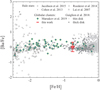 |
Fig. 8 Abundance of barium in the Galactic globular clusters (compilation by Marsakov et al. 2019) and Galactic field stars (thin and thick disk stars: Guiglion et al. 2018, halo stars: Lai et al. 2007; Cohen et al. 2013; Roederer et al. 2014; Jacobson et al. 2015). Average [Ba/Fe] ratio obtained in 261 RGB stars in 47 Tuc is marked by the red symbol where the 25th and 75th percentiles and the average values are indicated by the horizontal bars, while the extent of the whiskers correspond to the minimum and the maximum abundance values observed in this cluster. |
5.3 Implications for the chemical evolution scenarios of 47 Tuc
Results of the Ba abundance analysis in 261 RGB stars suggest that there have been no enrichment or depletion of Ba in the 2P stars of 47 Tuc. Similarly, no Ba–Na correlation was detected by D’Orazi et al. (2010) in their analysis of 110 RGB stars. These findings contradict the result obtained by Gratton et al. (2013), who observed a weak but statistically significant Ba–Na correlation in the sample of 114 RHB stars in 47 Tuc. However, as indicated by Grevesse et al. (2015), their detection of a possible Ba–Na correlation should be taken with caution because the [Na/O] correlation with effective temperature along the HB could partly (or even fully) explain the observed weak Ba-Na trend.
The obtained average barium-to-iron abundance ratio in 261 RGB stars in 47 Tuc,  , agrees well with the abundances obtained at this metallicity in other GGCs, as well as with those determined in the Galactic disc and halo stars (Fig. 8). This, along with the relatively narrow spread in Ba abundances of ± 0.06 dex (which can be fully accounted for by the Ba abundance determination error, σA(Ba) ≈ 0.12 dex), suggest thatBa abundance in 47 Tuc may reflect that of the primordial proto-cluster gas that has not been altered significantly (if at all) in the subsequent chemical enrichment during the evolution of the GGC.
In a recent analysis of Zr abundance in 237 RGB stars in 47 Tuc, Kolomiecas et al. (2021) detected a weak but statistically significant Zr–Na correlation and 2P–1P Zr abundance difference of 0.06 dex. Assuming that the 2P were indeed enriched in Zr but not in Ba would suggest that only some s-process elements were produced by the polluters that enriched the 2P stars in Na and modified abundances of other light elements such as Li, N, O, Mg, and Al, as determined in these earlier studies (see e.g. Bastian & Lardo 2018). Theoretical yields from low- and intermediate-mass AGB stars predict that Zr and Ba can be produced in substantial amounts but they ought to be synthesised simultaneously (Cristallo et al. 2015). Similarly, substantial amounts of Zr and Ba could be produced by explosive nucleosynthesis in massive rotating stars but, again, both elements should be produced simultaneously (Limongi & Chieffi 2018). Besides, in the latter scenario one would also expect some enrichment in the Fe-group and r-process elements that has not been observed in the Type I GGCs until now (e.g. Bastian & Lardo 2018; Gratton et al. 2019). It would be therefore very desirable to verify whether correlations between the other s-process and light chemical elements may exist in 47 Tuc as well as in other Type I GGCs.
6 Conclusions
We present homogeneous abundances of Fe, Na, and Ba determined in the sample of 261 RGB stars that belong to Galactic globular cluster (GGC) 47 Tuc. Contrary to the earlier finding of Gratton et al. (2013), our results show no statistically significant variation of Ba abundance with that of Na – thus suggesting that the primordial (Na-poor, 1P) and polluted (Na-rich, 2P) populations in this GGC are characterised by the same average Ba abundance,  (here, the error is standard deviation due to star-to-star abundance variation). This is also supported by the analysis of D’Orazi et al. (2010), who detected no Ba–Na correlation in a sample of 110 RGB stars in this GGC. Taken together with the recent finding of Kolomiecas et al. (2021), who reported a detection of weak but statistically significant Zr–Na correlation in 237 RG stars in 47 Tuc, these results would indicate that in this GGC the 2P stars may have been enriched in certain s-process elements (i.e. Zr) but not in others (i.e. Ba). It would therefore be very desirable to have the capacity to verify whether such correlations between the abundances of s-process and light chemical elements may exist in other GGCs via the analysis of more s-process elements in large samples of GGC stars, preferably by using spectra of higher resolution and a higher S/N.
Acknowledgements
We thank the anonymous referee for useful comments that significantly helped to improve the paper. This study has benefited from the activities of the “ChETEC” COST Action (CA16117), supported by COST (European Cooperation in Science and Technology) and from the European Union’s Horizon 2020 research and innovation programme under grant agreement No 101008324 (ChETEC-INFRA). J.K. acknowledges support from European Social Fund (project No 09.3.3-LMT-K-712-19-0172) under grant agreement with the Research Council of Lithuania. This work has made use of the VALD database, operated at Uppsala University, the Institute of Astronomy RAS in Moscow, and the University of Vienna.
Appendix A Differences between Ba abundances determined in different observing samples
As was indicated in Sect. 4, a number of target RGB stars have been observed in several observing programs (Table A.1). A comparison of Fe, Na, and Ba abundances obtained using spectra that were acquired in the different programs is provided in Fig. A.1–A.3. In most cases, differences between the average abundances obtained in various samples was very small and did not exceed 0.03 dex (Figs A.1-A.2).
Target stars common to different observing programs.
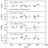 |
Fig. A.1 Comparison of the abundances (top three pannels) and microturbulence velocity values between the common stars in the programs 072.D-0777(A) and 073.D-0211(A). Grey dashed line shows average value of the difference. |
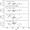 |
Fig. A.2 Comparison of the abundances (top three pannels) and microturbulence velocity values between the common stars in the programs 072.D-0777(A) and 088.D-0026(A). Grey dashed line shows average value of the difference. |
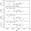 |
Fig. A.3 Comparison of the abundances (top three pannels) and microturbulence velocity values between the common stars in the programs 073.D-0211(A) and 088.D-0026(A). Grey dashed line shows average value of the difference. |
The final abundances of the target RGB stars were further corrected for these small systematic shifts. Since the program 072.D-0777(A) had the largest number of stars, we chose to apply abundance shifts relative to this sample. For stars in 073.D-0211(A) sample we applied abundance shifts of +0.03, +0.01, +0.03 dex for the abundances of Fe, Na, and Ba, respectively. In case of the sample 088.D-0026(A), abundances of Fe, Na, and Ba were corrected by +0.02, − 0.01, and − 0.03 dex, respectively.The final abundance ratios (Table D.1) were computed using So- lar referencevalues derived in Sect. 4.1.
Appendix B The Fe I and Fe II lines used in the abundance analysis
The list of Fe I and Fe II lines and their atomic parameters is provided in the Table B.1. We note that abundances from Fe II lines were only determined with the purpose of checking the agreement between the surface gravities obtained from photometry and those derived using Fe II lines; however, they were not used in further analysis. Thus, Fe abundances used throughout this paper are those that were obtained using Fe I lines.
List of iron spectral lines used in the abundance determination.
Appendix C Abundances of Ba in the target RGB stars with 4600 < Teff < 4700 K
As noted inSect. 5, our data hint to a weak Ba–Na anti-correlation. Further analysis hasrevealed that this may be an artefact caused by several spurious outliers with 4600 < Teff < 4700 K that were observed in one of the programs, 073.D-0211(A) (Fig. C.1). No such anti-correlation is seen in any other ΔTeff = 100 K wide effective temperature bins. Indeed, no statistically significant anti-correlation is left in the 4600 < Teff < 4700 K either when stars 19992, 38289, and 21369 are excluded. We therefore conclude that there is no statistically significant Ba–Na correlation in the analysed sample of 261 RGB stars in 47 Tuc.
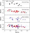 |
Fig. C.1 Barium and sodium abundances in the effective temperature range 4600 < Teff < 4700 K. Labels next to the outlying data points show identifications of the stars. |
Appendix D Abundances of Fe, Na, and Ba in 261 target RGB stars in 47 Tuc
Abundancesof Fe (LTE), Na (NLTE), and Ba (NLTE) obtained in 261 RGB stars in 47 Tuc are provided in Table D.1.
Abundances of Fe, Na, and Ba determined in the sample of 261 stars in 47 Tuc. In cases when abundances were determined using data from several observing programs, microturbulence velocities and abundances obtained using spectra from each individual program are provided. The IDs of individual stars and IDs of the corresponding observing programs are given in the last two columns, respectively (072.D-0777(A), PI: P. François; 073.D-0211(A), PI: E. Carretta; 088.D-0026(A), PI: I. McDonald). The complete table is available in electronic form.
References
- Alonso, A., Arribas, S., & Martínez-Roger, C. 1999, A&AS, 140, 261A [NASA ADS] [CrossRef] [EDP Sciences] [Google Scholar]
- Andrievsky, S. M., Spite, M., Korotin, S. A., et al. 2009, A&A, 494, 1083 [NASA ADS] [CrossRef] [EDP Sciences] [Google Scholar]
- Barklem, P. S., Belyaev, A. K., Dickinson, A. S., et al. 2010, A&A, 519, A20 [NASA ADS] [CrossRef] [EDP Sciences] [Google Scholar]
- Bastian, N., & Lardo, C. 2018, ARA&A, 56, 83 [Google Scholar]
- Baumgardt, H., Hilker, M., Sollima, A., & Bellini, A. 2019, MNRAS, 482, 5138 [Google Scholar]
- Bergbusch, P. A., & Stetson, P. B. 2009, AJ, 138, 1455 [NASA ADS] [CrossRef] [Google Scholar]
- Bonifacio, P., Pasquini, L., Molaro, P., et al. 2007, A&A, 470, 153 [NASA ADS] [CrossRef] [EDP Sciences] [Google Scholar]
- Caffau, E., Ludwig, H.-G., Steffen, M., Freytag, B., & Bonifacio, P. 2011, Sol. Phys., 268, 255 [Google Scholar]
- Carlsson, M. 1986, UppOR, 33 [Google Scholar]
- Carretta, E., Bragaglia, A., Gratton, R. G., G., et al. 2009, A&A, 505, 117 [NASA ADS] [CrossRef] [EDP Sciences] [Google Scholar]
- Černiauskas, A., Kučinskas, A., Klevas, J., et al. 2018, A&A, 616, A142 [NASA ADS] [CrossRef] [EDP Sciences] [Google Scholar]
- Cohen, J. G., Christlieb, N., Thompson, I., et al. 2013, ApJ, 778, 56 [Google Scholar]
- Cristallo, S., Straniero, O., Piersanti, L., & Gobrecht, D. 2015, ApJS, 219, 40 [Google Scholar]
- D’Antona, F., Vesperini, E., D’Ercole, A., et al. 2016, MNRAS, 458, 2122 [Google Scholar]
- Decressin, T., Charbonnel, C., Siess, L., et al. 2007, A&A, 505, 727 [Google Scholar]
- Denisenkov, P. A., & Hartwick, F. D. A. 2014, MNRAS, 437, L21 [NASA ADS] [CrossRef] [Google Scholar]
- Dobrovolskas, V., Kučinskas, A., Bonifacio, P., et al. 2014, A&A, 576, A128 [Google Scholar]
- D’Orazi, V., Gratton, R., Lucatello, S., et al. 2010, ApJ, 719, L213 [CrossRef] [Google Scholar]
- D’Orazi, V. D., Campbell, S. W., Lugaro, M., et al. 2013, MNRAS, 433, 366 [CrossRef] [Google Scholar]
- Doyle, A. P., Davies, G. R., Smalley, B., Chaplin, W. J., & Elsworth, Y. 2014, MNRAS, 444, 3592 [Google Scholar]
- Gaia Collaboration (Brown, A. G. A., et al.) 2021, A&A, 649, A1 [NASA ADS] [CrossRef] [EDP Sciences] [Google Scholar]
- Gallagher, A. J., Bergemann, M., Collet, R., et al. 2020, A&A, 634, A55 [NASA ADS] [CrossRef] [EDP Sciences] [Google Scholar]
- Gieles, M., Charbonnel, C., Krause, M. G. H., et al. 2018, MNRAS, 478, 2461 [Google Scholar]
- Gratton, R. G., Lucatello, S., Sollima, A., et al. 2013, A&A, 549, A41 [NASA ADS] [CrossRef] [EDP Sciences] [Google Scholar]
- Gratton, R. G., Bragaglia, A., Carretta, E., et al. 2019, A&ARv, 27, 8 [Google Scholar]
- Grevesse, N., Scott, P., Asplund, M., & Sauval, A. J. 2015, A&A, 573, A27 [NASA ADS] [CrossRef] [EDP Sciences] [Google Scholar]
- Guiglion, G., de Laverny, P., Recio-Blanco, A., & Prantzos, N. 2018, A&A, 619, A143 [NASA ADS] [CrossRef] [EDP Sciences] [Google Scholar]
- Jacobson, H. R., Keller, S., Frebel, A., et al. 2015, ApJ, 807, 171 [NASA ADS] [CrossRef] [Google Scholar]
- James, G., François, P., Bonifacio, P. F., et al., 2004, A&A, 427, 825 [NASA ADS] [CrossRef] [EDP Sciences] [Google Scholar]
- Kim, Y.-C., Demarque, P., Yi, S. K., & Alexander, D. R. 2002, ApJS, 143, 499 [Google Scholar]
- Kolomiecas, E., Dobrovolskas, V., Kučinskas, A., Bonifacio, P., & Korotin, S. 2021, A&A, submitted [NASA ADS] [CrossRef] [EDP Sciences] [Google Scholar]
- Korotin, S. A., Andrievsky, S. M., & Luck, R. E. 1999, A&A, 351, 168 [NASA ADS] [Google Scholar]
- Korotin, S., Mishenina, T., Gorbaneva, T., & Soubiran, C. 2011, MNRAS, 415, 2093 [NASA ADS] [CrossRef] [Google Scholar]
- Kučinskas, A., Dobrovolskas, V., & Bonifacio, P. 2014, A&A, 568, L4 [NASA ADS] [CrossRef] [EDP Sciences] [Google Scholar]
- Kupka, F., Ryabchikova, T. A., Piskunov, N. E., Stempels, H. C., & Weiss, W. W. 2000, BaltA, 9, 590 [NASA ADS] [Google Scholar]
- Kurucz, R. L. 1993, ATLAS9 Stellar Atmosphere Programs and 2 km/s Grid, CD-ROM No.13 (Cambridge, Mass.: Smithsonian Astrophysical Observatory) [Google Scholar]
- Kurucz, R. L., Furenlid, I., Brault, J., & Testerman, L. 1984, Solar Flux Atlas from 296 to 1300 nm (Sunspot, New Mexico: National Solar Observatory) [Google Scholar]
- Lai, D. K., Johnson, J. A., Bolte, M., et al. 2007, ApJ, 667, 1185 [NASA ADS] [CrossRef] [Google Scholar]
- Lodders, K. 2021, Space Sci. Rev., 591, 1220 [Google Scholar]
- Limongi, M., & Chieffi, A. 2018, ApJS, 237, 13 [NASA ADS] [CrossRef] [Google Scholar]
- Marino, A. F., Milone, A. P., Karakas, A. I., et al. 2015, MNRAS, 450, 815 [NASA ADS] [CrossRef] [Google Scholar]
- Marino, A. F., Milone, A. P., Renzini, A., et al. 2019, MNRAS, 487, 3815 [CrossRef] [Google Scholar]
- Marsakov, V. A., Koval, V. V., & Gozha, M. L. 2019, Astron. Rep., 63, 274 [NASA ADS] [CrossRef] [Google Scholar]
- Mashonkina, L. I., & Bikmaev, I. F. 1996, Astron. Rep., 40, 94 [NASA ADS] [Google Scholar]
- Milone, A. P., Marino, A. F., Mastrobuono-Battisti, A., & Lagioia, E. P. 2018, MNRAS, 479, 5005 [NASA ADS] [CrossRef] [Google Scholar]
- Pasquini, L., Bonifacio, P., Molaro, P., et al. 2005, A&A, 441, 549 [NASA ADS] [CrossRef] [EDP Sciences] [Google Scholar]
- Ramírez, I., & Meléndez, J. 2005, ApJ, 626, 465 [Google Scholar]
- Roederer, I. U., Preston, G. W., Thompson, I. B., et al. 2014, AJ, 147, 136 [Google Scholar]
- Ryabchikova, T., Piskunov, N., Kurucz, R. L., et al. 2015, Phys. Scr., 90, 054005 [Google Scholar]
- Sbordone, L. 2005, Mem. Soc. Astron. It., 8, 61 [Google Scholar]
- Sbordone, L., Bonifacio, P., Castelli, F., & Kurucz, R. L. 2004, Mem. Soc. Astron. It., 5, 93 [Google Scholar]
- Scott, P., Asplund, M., Grevesse, N., Bergemann, M., & Sauval, A. J. 2015, A&A, 573, A25 [NASA ADS] [CrossRef] [EDP Sciences] [Google Scholar]
- Shen, Z.-X., Bonifacio, P., Pasquini, L., et al. 2010, A&A, 524, L2 [NASA ADS] [CrossRef] [EDP Sciences] [Google Scholar]
- Spite, M., Spite, F., Gallagher, A. J., et al. 2016, A&A, 594, A79 [NASA ADS] [CrossRef] [EDP Sciences] [Google Scholar]
- Thygesen, A. O., Sbordone, L., Andrievsky, S., et al. 2014, A&A, 572, A108 [NASA ADS] [CrossRef] [EDP Sciences] [Google Scholar]
- Tody, D. 1986, Proc. SPIE, 627, 733 [NASA ADS] [CrossRef] [Google Scholar]
- Trager, S. C., Djorgovski, S., & King, I. R. 1993, ASPC Conf. Ser., 50, 347 [Google Scholar]
- Tsymbal, V. 1996, ASP Conf. Ser., 108, 198 [Google Scholar]
- Villanova, S., & Geisler, D. 2011, A&A, 535, A31 [NASA ADS] [CrossRef] [EDP Sciences] [Google Scholar]
- Wiese, W. L., & Martin, G. A. 1980, in Wavelengths and transition probabilities for atoms and atomic ions: Part 2, Transition probabilities, NSRDS-NBS, Vol. 68 [Google Scholar]
- Worley, C. C.,& Cottrell, P. L. 2012, PASA, 29, 29 [NASA ADS] [CrossRef] [Google Scholar]
- Worley, C. C., Cottrell, P. L., McDonald, I., & van Loon, J. Th. 2010, MNRAS, 402, 2060 [NASA ADS] [CrossRef] [Google Scholar]
All Tables
[Ba/Fe]−[Na/Fe] abundance correlation coefficients and their in the full sample of 261 RGB stars in 47 Tuc and sub-samples divided into ΔTeff = 100 K-wide bins.
Abundances of Fe, Na, and Ba determined in the sample of 261 stars in 47 Tuc. In cases when abundances were determined using data from several observing programs, microturbulence velocities and abundances obtained using spectra from each individual program are provided. The IDs of individual stars and IDs of the corresponding observing programs are given in the last two columns, respectively (072.D-0777(A), PI: P. François; 073.D-0211(A), PI: E. Carretta; 088.D-0026(A), PI: I. McDonald). The complete table is available in electronic form.
All Figures
|
Fig. 1 Target RGB stars in the Teff − logg
plane. The red line is Yonsei-Yale (Kim et al. 2002) isochrone (12 Gyr, |
| In the text | |
|
Fig. 2 Examples of the observed (black dots) and best-fitted synthetic Na I line profiles (red lines) in the GIRAFFE spectra of the target stars characterised by different Na abundances and effective temperatures (Teff ≈ 4250 K, top row; Teff ≈ 4750 K, bottom row). The continuum level is shown as the gray dashed line. |
| In the text | |
|
Fig. 3 Fe (top row), Na (middle row), and Ba (bottom row) abundances plotted against the microturbulence velocity (left column) and effective temperature (right column). In all panels, the linear fits to the data are shown as the solid red lines. |
| In the text | |
|
Fig. 4 Examples of the observed (black dots) and best-fitted synthetic spectra in the vicinity of the 614.17 nm Ba II line (red lines) in the GIRAFFE spectra of the target stars characterised by different effective temperatures (Teff ≈ 4250 K, top panel; Teff ≈ 4750 K, bottom panel). The continuum level is shown as the gray dashed line. |
| In the text | |
|
Fig. 5 [Ba/Fe] abundance ratios determined in 261 RGB stars in 47 Tuc, plotted versus their [Na/Fe] abundance rations. Typical abundance error bars are shown in the bottom left corner. The linear fit to the data is shown as the solid red line. |
| In the text | |
|
Fig. 6 [Ba/Fe] abundance ratios obtained in 261 RGB stars in 47 Tuc, plotted versus relative radial distance from the cluster center. Cluster half-mass radius, rh = 174 arcsec, was taken from Trager et al. (1993). Linear fit to the data is marked as the solid red line. Typical abundance error is shown as the vertical bar in the bottom left corner. |
| In the text | |
|
Fig. 7 Absolute abundances of Ba and Na in the A(Ba) − A(Na) plane. Typical abundance error bars are shown in the bottom left corner. The linear fit to the data is shown as the solid red line. |
| In the text | |
|
Fig. 8 Abundance of barium in the Galactic globular clusters (compilation by Marsakov et al. 2019) and Galactic field stars (thin and thick disk stars: Guiglion et al. 2018, halo stars: Lai et al. 2007; Cohen et al. 2013; Roederer et al. 2014; Jacobson et al. 2015). Average [Ba/Fe] ratio obtained in 261 RGB stars in 47 Tuc is marked by the red symbol where the 25th and 75th percentiles and the average values are indicated by the horizontal bars, while the extent of the whiskers correspond to the minimum and the maximum abundance values observed in this cluster. |
| In the text | |
|
Fig. A.1 Comparison of the abundances (top three pannels) and microturbulence velocity values between the common stars in the programs 072.D-0777(A) and 073.D-0211(A). Grey dashed line shows average value of the difference. |
| In the text | |
|
Fig. A.2 Comparison of the abundances (top three pannels) and microturbulence velocity values between the common stars in the programs 072.D-0777(A) and 088.D-0026(A). Grey dashed line shows average value of the difference. |
| In the text | |
|
Fig. A.3 Comparison of the abundances (top three pannels) and microturbulence velocity values between the common stars in the programs 073.D-0211(A) and 088.D-0026(A). Grey dashed line shows average value of the difference. |
| In the text | |
|
Fig. C.1 Barium and sodium abundances in the effective temperature range 4600 < Teff < 4700 K. Labels next to the outlying data points show identifications of the stars. |
| In the text | |
Current usage metrics show cumulative count of Article Views (full-text article views including HTML views, PDF and ePub downloads, according to the available data) and Abstracts Views on Vision4Press platform.
Data correspond to usage on the plateform after 2015. The current usage metrics is available 48-96 hours after online publication and is updated daily on week days.
Initial download of the metrics may take a while.