| Issue |
A&A
Volume 656, December 2021
|
|
|---|---|---|
| Article Number | A145 | |
| Number of page(s) | 18 | |
| Section | Interstellar and circumstellar matter | |
| DOI | https://doi.org/10.1051/0004-6361/202039787 | |
| Published online | 17 December 2021 | |
YY Hya and its interstellar environment
1
Institut für Astro- und Teilchenphysik, Leopold–Franzens Universität Innsbruck,
Technikerstr. 25,
6020
Innsbruck,
Austria
e-mail: This email address is being protected from spambots. You need JavaScript enabled to view it.
2
Instituto de Astronomía, Universidad Católica del Norte,
Av. Angamos 0610,
Antofagasta,
Chile
3
Department of Physics and Astronomy,
6127 Wilder Laboratory, Dartmouth College,
Hanover,
NH
03755-3528,
USA
4
Sternwarte Bärenstein,
Feldstraße 17,
09471
Bärenstein,
Germany
5
Montfraze,
01370
Saint Etienne Du Bois,
France
6
Leopoldo Stadtlober Street 49,
89871-000
Serra Alta,
Brazil
7
Department of Physics and Astronomy, Purdue University,
525 Northwestern Avenue,
West Lafayette,
IN
47907
USA
8
MDM Observatory, Kitt Peak National Observatory,
950 N. Cherry Ave.,
Tucson,
AZ
85719,
USA
Received:
29
October
2020
Accepted:
8
October
2021
Abstract
Context. During a search for previously unknown Galactic emission nebulae, we discovered a faint 36′ diameter Hα emission nebula centered around the periodic variable YY Hya. Although this star has been classified as an RR-Lyr variable, such a classification is inconsistent with a Gaia distance of ≃450 pc. The GALEX image data also show YY Hya as having a strong UV excess, suggesting the existence of a hot and compact binary companion.
Aims. We aim to clarify the nature of YY Hya and its nebula.
Methods. In addition to our discovery image data, we obtained a 2.°5 × 2.°5 image mosaic of the whole region with CHILESCOPE facilities and time-series spectroscopy at MDM observatory. Also, we used data from various space missions to derive an exact orbital period and a spectral energy distribution.
Results. We find that YY Hya is a compact binary system containing a K dwarf star that is strongly irradiated by a hot white dwarf companion. The spectral characteristics of the emission lines that are visible only during the maximum light of the perfectly sinusoidal optical light curve show signatures resembling those of members of the BE UMa variable family. These are post-common-envelope pre-cataclysmic variables. However, the companion star here is more massive than that found in other group members and, thus, the progenitor of the white dwarf must have been a star between 3 and 4 M⊙. The nebula appears to be an ejected common-envelope shell with a mass on the order of one M⊙ and an age of 500 000 yr. This makes it the biggest such shell known thus far. The alignment of neighboring nebulosities some 45′ to the northeast and southwest of YY Hya suggests that the system has had strong bipolar outflows. We also briefly speculate that it might be related to the 1065 BP “guest-star” reported in ancient Chinese records.
Key words: novae, cataclysmic variables / white dwarfs / evolution / stars: individual: YY Hya
© ESO 2021
1 Introduction
In a systematic search for previously unrecognized Galactic nebulosities on sky survey plates downloaded from the SuperCOSMOS facility archive in Edinburgh1 (Hambly et al. 2001), we discovered a small bow-like emission structure near α(J2000) = 09:25:50, δ(J2000) = − 22:23:00. Follow-up images taken with a small telescope facility at Serra Alta, Brazil showed that this feature is the brightest part of a much larger (36′ diameter), highly structured, and nearly circular Hα nebula centered on the variable star YY Hya (α = 09:26:20.596, δ = − 22:23:38.38; l = 252°.81, b = +19°.94). We also found two additional emission structures, located ~45′ northeast and southwest of the center (see Fig. 1). The initial assumption was that it is a possible planetary nebula (PN) and it was assigned the identifier StDr Object 20 (PN G252.8+19.9) in the HASH PN data base (Parker et al. 2016, 2017).
In summary, YY Hya was discovered nearly 85 yr ago as Harvard Variable No. 7525 (Boyce 1936) and classified as an RR Lyr star, called a “cluster” variable in the literature at that time. Guthnick & Prager (1936) assigned the name YY Hya shortly afterthat. Drake et al. (2017), using data from the Catalina Real-time Transient Survey (CRTS, Drake et al. 2009), determined a period of 0.33479 d, and classified the star as a c-type RR Lyr (RRc), based on its almost perfectly sinusoidal light curve and high amplitude of nearly one magnitude. The RRc classification implies an absolute magnitude range from 0m.85 < MV < 0m.55 (Catelan et al. 2004; Dambis et al. 2013). This led to an initial distance estimate of 4.05 < DRR < 4.75 kpc.
However, recent parallax measurements indicate a much shorter distance that would be inconsistent with any kind of RR Lyr star. The inverse of the parallax from Data Release 2 (DR2) of the Global Astrometric Interferometer for Astrophysics (Gaia; Gaia Collaboration 2018) is 443 ± 6 pc – about ten times smaller than that expected for an RR Lyr star. The more recent Gaia Early Data Release 3 (EDR3; Gaia Collaboration 2021) gives 456 ± 3 pc. Although this new value does not overlap within the 1σ errors with the DR2 result, we adopted that value as it is based on more extensive data and has correspondingly smaller uncertainties. However, up to now, the Gaia analysis has only solved for the star’s position, parallax, and proper motions. Its motions due to binary orbits have not yet been included in Gaia as a source of possible systematic errors. However, in the case of the system here as we see later, the whole orbit extends only to 0.03 mas. That is about 1σ of the given parallax error in Gaia eDR3. Thus, the distance from Gaia still seems to be reliable, however, the orbital motion might be the causefor the significant shift between the two major data releases and so, the realistic error, assuming some systematic component, is more likely on the order of 10 pc.
In this paper, we present follow-up imaging and time-series spectroscopy, along with photometric data collected from various literature and data base resources, as well as an analysis of photometry from the Transiting Exoplanet Survey Satellite (TESS, Ricker et al. 2015). We used these data to classify the system using radial velocities, spectral energy distribution (SED), and the UV excess found by the Galaxy Evolution Explorer (GALEX, Bianchi 1999). We furthermore put the kinematic behavior of the system into the Galactic context and derived detailed parameters for the progenitor stars. Finally, we discuss a possible link to a medieval “guest-star” observation reported by Chinese observers in this direction on the sky (Hsi 1957; Ho 1962).
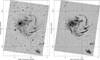 |
Fig. 1 Hα image taken at Serra Alta, Brazil of the region around YY Hya. Left: original image. Right: image following the star removal procedure (see text). The inner main nebula has a diameter of 36′. In the northeast and southwest corners, the vis-à-vis emission structures are clearly visible, both 47′ from the variable star. Northeast structure is just at the image edge and partly cut off. |
2 Data and reductions
2.1 Hα imaging
The Hα discovery images were taken in January 2020 in Serra Alta, Brazil2, using a 115mm F7 TS Proline Triple APO refractor from Teleskop–Service Ransburg3 along with a focal reducer, resulting in a final f/5.5 The detector was a ZWO4 Camera ASI 1600 MM-Cool equipped with a 4656 × 3520, 3.8 μm pixel CMOS Panasonic MN34230 and an OPTOLONG5 7 nm wide Hα filter. This resulted in a pixel scale of 1′′.24 pixel−1 and a field of view (FOV) of 1°.6 × 1°.21.
The image shown in Fig. 1 is a composite of 120 × 600 s exposures for a total exposure time of 20 h. A set of matching broadband red filter images were also obtained in order to remove the stellar background. These red filter images were stretched manually by a nonlinear intensity curve to correct for differences in the calibration and finally subtracted from the Hα image.
The resulting images shows a highly structured Hα nebula with a diameter of ~36′. In addition,two smaller nebulosities in opposite directions roughly 45′ to the northeast and southwest from YY Hya are also visible. Examination of copies of the original photographic sky surveys ESO-R (West 1974) shows no more evidence for the nebula other than the small southwestern arc than already seen on the H-compressed digital scans. Likewise, no part of th e nebula is visible at the SERC-J (Morgan 1995) plate copy, suggesting that the nebula does not have a significant [O III] emission.
To investigate further, we booked time at the CHILESCOPE remotely controlled commercial observatory facilities. Details on the location, the instrumentation used and the calibration are given in Appendix B. Images with Hα, [O III], and [S II] filters from Astrodon6 were obtained. However, 30 min of exposure in the [O III] and [S II] bands centered at the main nebula showed no detection of even the brightest filaments. Thus, the campaign, lasting from March 9 to June 13 2021, was ultimately focused entirely on the Hα imaging. The aim was the full coverage of the field and the possible detection of further distant structures and a calibrated intensity estimate. However, besides the already mentioned structures, no other distant structures related YY Hya and its nebula could be identified. Figure 2 shows the mosaic of the 294 Hα images with1200 s exposure time each (98 h integration time). The brightest nebular filaments are about 4 × 10⁻¹⁷ erg cm−2 s−1 arcsec−2. The faintest visible structures at 1.5σ to the background rms of single pixels are around 8 10−18 erg cm−2 s−1 arcsec−2.
Higher resolution images were also obtained with the 2.4 m Hiltner telescope at the MDM Observatory at Kitt Peak, Arizona using the Ohio State Multi-Object Spectrograph (OSMOS; Martini et al. 2011) in direct imaging mode. A 4 k × 4 k CCD provided an effective FOV of 18′× 18′. With 2 × 2 on-chip binning, this yielded an image scale of 0.546′′ pixel−1. A series of narrow passband Hα + [N II], [O III] λ5007, and [S II] filter images were taken of the northeastern and southwestern outlying nebulosities with exposure times of 600–1200 s. The resulting Hα images of the NE and SW outlying nebulae are shown in Fig. 3. The sharp filamentary appearance of the emission along with the lack of appreciable [O III] and [S II] emissions strongly suggests these filaments are Balmer-dominated shock filaments with shock velocities ≃100 km s−1 or more, depending on the density of the ambient interstellar medium.
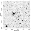 |
Fig. 2 Hα image mosaic obtained at CHILESCOPE with a linear gray-scale mapping with surface brightness from zero to 1.5 10−16 erg cm−2 s−1 arcsec−1. The stellar limiting magnitude is about Gaia RP ≈ 21m. 8. The round nebula southwards is not related to our target but the beforehand known planetary nebula StDr 47 (PN G253.7+19.4, 09h27m31s. 46, −23°22′34″.40). |
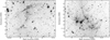 |
Fig. 3 MDM Hα images of the northeastern (left) and southwestern (right) outlying nebulosities around YY Hya showing the presence of emissions of overlapping shocks. |
2.2 UV images
UV GALEX images (Bianchi 1999; Martin et al. 2005) were obtained from the online data bases. This nearly all-sky UV imaging survey used wide-band filters centered around 154.9 and 230.5 nm, called FUV and NUV, respectively. The full-resolution images contain mainly pixels with individual photons in about 30% of the pixels and more than 60% of the image pixels containing no photons at all. Simply averaging these images would have artificially enhanced the intensity in the overlap regions of the individual pointings, while the use of a smoothing filter would degrade the brighter parts of the image. We therefore used a nearest-neighbor algorithm in the way that is normally used for investigations of stellar cluster density (Gao 2016), which preserves the faint background without touching the brighter regions. Seven survey fields were combined in that way to get a larger mosaic for the final image (Fig. 4).
Interestingly, only the far NE and SW pair of nebulae ~45′ from the center are clearly detected in the GALEX images. The average position angle of these features is 25° (north over east) on the sky. This is consistent with these outer emissions as being due to shocks, as suggested by the optical images. A very weak hint of parts of the main nebula in a large “S” shaped structure is visible. Although GALEX images show many reflection ghost images, the detection of the lobes in the GALEX images is convincing as the features are neither in the mirroring direction along the optical axes from other bright sources, nor are they in the image of the same telescope pointing as YY Hya. They also resemble in basic shape and location the outer nebulae seen in the optical images. The FUV/NUV ≫ 1 suggests similar physics of shocked gas like found in the 4 pc wide blue ring nebula around TYC 2597-735-1 (Hoadley et al. 2020).
2.3 Optical and infrared photometry
The light curve data from of the Catalina Real-time Transient Survey CRTS (Drake et al. 2009) were downloaded from the online data base7 and converted to the solar system barycentric time frame. Additionally, we obtained the time-series photometry from the Gaia DR2 data base (Holl et al. 2018). The WISE data and a handful of data points available from the Palomar Transient Factory (PTF, Law et al. 2009) were obtained from the NASA/IPAC Infrared Science Archive (IRSA)8.
Furthermore, we loaded the Transiting Exoplanet Survey Satellite (TESS, Ricker et al. 2015) full-frame images (FFI) of sector 8 (February 2020) along with the quick-look, early release of calibrated FFIs of sector 35 (February/March 2021), and we derived the simple aperture photometry (SAP) flux light curve by using eleanor (Feinstein et al. 2019) and our in-house public tool smurfs9. As the TESS pixels are very large (21′′), the source is contaminated in the SAP aperture by the slightly brighter star Gaia DR2 5675391264067546624, with G = 13m.3697 and a color BP-RP = 0m.6597, which are very similar to that of YY Hya. Thus, while this data allows for a time-series analysis, no absolute calibration of the magnitude and the amplitude is possible. We thus used the red Gaia RP, with nearly the same effective wavelength of the passband (see Table A.2) to derive the calibration scale factor.
Using the visual band magnitude and color of the star in the Gaia photometry to estimate a spectral class range and the apparent magnitude, the central stellar source in the GALEX DR5 source data base (Bianchi et al. 2012) at the position of YY Hya shows a clear UV excess. In total, the collection of time series spans 16 yr and 16 802 periods. A complete summary of the photometry can be found in Table A.1. We searched the time series for periods using our own implementation of the phase-dispersion minimization (PDM, Stellingwerf 1978) algorithm. Global solutions as well as individual blocks of two years were obtained to identify possible period changes, but no such changes were found down to the 0.5σ level. The period, P = 0.d3347894 ± 0.d0000004 (≡ to a frequency f = 2.98695 d−1), is constant to better than 0.1 s during those 16 yr. Comparing the formalism from Knigge et al. (2011), the resulting limit of the period change implies that the system does not show strong mass transfer at the moment. The PDM is very sensitive to general period changes on those long time series. But as shown for the case of WZ Sge by Patterson et al. (2018) and as discussed in there for a set of other system as well, these stars often show wiggles of the observed-computed (O–C) timing of eclipses, typically on timescales of 10–30 yr. As we do not see an eclipse in our system, we are not sensitive to such small changes here. The ephemeris of minimum sinusoidal optical light curve is
 (1)
(1)
where E is the integer cycle count.
Even more surprising is the remarkably sinusoidal shape of the light curve. Fitting a single sine function gives for the TESS data a correlation coefficient of R2 ≿ 0.9997 and rms = 0m.0073. The near-perfect sinusoidal light curve allowed us to normalize the amplitudes from various wavelengths to a common light curve, showing that this perfect sinusoidal behavior was valid throughout the whole data period (Fig. 5). Moreover, after the drop from a flux ratio between maximum and minimum of the optical light curve of 2.5 for the two blue bands around 500–2.2 at 600 nm the amplitude is fairly well linear with a very small slope from 2.2 to 1.95 from approximately 610–4600 nm. As the flux in the Rayleigh–Jeans approximation part of a spectrum depends linearly on temperature T, this suggests that the variability originates mostly from temperature changes similar to those found in irradiated systems (Schaffenroth et al. 2019). Near infrared (NIR) data obtained at two epochs by the Deep Near Infrared Southern Sky Survey (DENIS, Epchtein et al. 1997) and one epoch from the Two Micron All Sky Survey (2MASS, Skrutskie et al. 1997) exist. All were obtained at phases near minimum. Using the linear relation of the amplitude with wavelength from the data with existing light curve small corrections towards an estimated minimum light were obtained to be used for the SED based on ATLAS9 stellar atmospheres (Castelli & Kurucz 2003) later. As the NIR observations were obtained near minimum such an estimate for observations at maximum light would be too much of an extrapolation. Thus we did not use the NIR photometry for the SED during maximum. The filter definitions and the calibration zero points for the entire photometric data are given in Table A.2.
Using the newest 3D Galactic extinction map Bayestar2019 (Green et al. 2019), we derived an interstellar reddening as low as E(B − V) = 0m.02, while the Stilism map (Lallement et al. 2019)gives a value of E(B − V) = 0m.043 ± 0m.17. We thus adopted the mean value of 0m.032 for our subsequent investigations. Furthermore, we adopted the extinction curve by Cardelli et al. (1989) to cover solely the extinction of the foreground and the environment (as any possible internal extinction within the system itself cannot be detected that way).
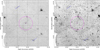 |
Fig. 4 GALEX FUV (left) and GALEX NUV (right) composite mosaic image. The 36′ circle and the two 47′ arcs are centered with respect to the position of YY Hya. While the central nebula is not clearly detected, the two vis-à-vis emission lobes are clearly visible in both bands. |
2.4 Optical spectra
We obtained spectra for YY Hya at the 2.4 m Hiltner telescope at the MDM Observatory at Kitt Peak, Arizona, using the Ohio State Multi-Object Spectrograph (OSMOS; Martini et al. 2011). A 1′′.4 slit and a blue grism yielded a resolution of R ≈ 1600 and a wavelength coverage from 3975 to 6865 Å. For the wavelength calibration, we used Hg, Ne, and Ar comparison lamps and fine-tuned the wavelength scale using night-sky emission features as needed. We observed spectrophotometric standard stars for flux calibration. Reductions were accomplished using an own pipeline that included elements from astropy and IRAF/pyraf. We also obtained a few spectra with the 1.3 m McGraw-Hill telescope and modspec spectrograph. These had apoorer signal-to-noise ratio (S/N) than the 2.4 m data, but which was nonetheless consistent with the results.
Table 1 summarizes the observations. A few spectra were taken on three successive nights in 2020 December, all of them near maximum in the optical light curve (the period is so close to 1/3 day that observations on successive nights near meridian transit are at nearly the same phase). In 2021 February and March, we obtained much more extensive data on more widely separated nights, which sampled the entire orbit.
In the upper panel of Fig. 6, the averages of the flux-calibrated OSMOS spectra from near maximum and minimum inthe optical light curve are plotted on the same scale. The maximum-light spectrum is dominated by a strong blue continuum and numerous emission lines of H, He I, He II and weaker features that appear to be mostly singly and doubly ionized C and N. The latter are very narrow while the H and He lines appear to be Stark broadened.
This kind of mixture of wide and strong H and He lines combined with narrow emission lines of low-ionized CNO elements looks very much like that of spectra found in post-common-envelope pre-cataclysmic variables like EC 11575-1845 (= TW CrV), V664 Cas (the central star of the planetary nebula HFG 1, Exter et al. 2005), HS 1857+5144 (Aungwerojwit et al. 2007; Shimansky et al. 2009), BE UMa (Shimansky et al. 2008), NN Ser (the central star of the PN G068.1+11.0, Parsons et al. 2010; Mitrofanova et al. 2016). However, the emission-to-continuum line contrast is much weaker in those objects than the one we find here. Also, they all show spectra signatures of a white dwarf (WD) companion in the optical and have late M-type star companions (except for BE UMa, Shimansky et al. 2008). In addition, UU Sge, also belonging to that class of objects, shows predominately much higher ionization levels for the CNO elements in the spectra (Wawrzyn et al. 2009).
In Table B.1, we give a full listing including relative line strengths of the very rich emission spectrum at phase 0.5. The minimum-light spectrum is much fainter overall, with much weaker emission lines and prominent absorption features of alate-type star.
To quantify the contribution of the late-type star, we used a set of spectra of late-type stars classified by Keenan & McNeil (1989), observed with the modspec. Using an interactive program we scaled various spectra from this set and subtracted them from the minimum-light spectra, varying the spectral type and scale factor to optimize the cancellation of the late-type absorption features. The lower panel of Fig. 6 shows the best result, obtained with a K2 V star. Stars within ± 2 subclasses of this gave acceptable cancellations.
We measured radial velocities of the late-type star using the IRAF fxcor task, which implements cross-correlation methods, as described by Tonry & Davis (1979). As a template, we used the average of 76 spectra of late-type IAU velocity standards that had been shifted to zero apparent velocity before the cross-correlation. We note that in this method, the wavelengths of individual features are not measured. Regions around emission lines were masked. The spectra near minimum light gave strong correlations. Near maximum, in which the late-type features were barely visible, the correlations were much weaker and the velocity uncertainties correspondingly larger, but nearly all spectra showed at least some correlation. We also measured the velocity of the Hα emission line, using a convolution technique (Schneider & Young 1980); the velocities of the other emission lines were similar.
Figure 7 shows the velocities folded with the photometric phase. The emission lines move nearly in phase with the absorption, but with a somewhat smaller velocity amplitude. Table 2 gives the parameters of the best fitting sinusoids of the form ![Mathematical equation: $v(t) = \gamma + K_{\textrm{em,abs}}^i \sin[2 \pi(t - T_0)/P]$](/articles/aa/full_html/2021/12/aa39787-20/aa39787-20-eq2.png) , such that T0 corresponds to inferior conjunction of the moving object. The period was held fixed at the photometric value, which spans a much longer time base; the epochs T0 were permitted to vary. Even with this, both the epochs in Table 2 align with the ephemeris in Eq. (1) to within 0.01 cycles. Equation (1) is for minimum light. The velocities therefore indicate an irradiation effect, since the cool star’s heated face is maximally turned away from us at an inferior conjunction.
, such that T0 corresponds to inferior conjunction of the moving object. The period was held fixed at the photometric value, which spans a much longer time base; the epochs T0 were permitted to vary. Even with this, both the epochs in Table 2 align with the ephemeris in Eq. (1) to within 0.01 cycles. Equation (1) is for minimum light. The velocities therefore indicate an irradiation effect, since the cool star’s heated face is maximally turned away from us at an inferior conjunction.
In Figs. 8 and 9, we present phase-resolved spectra similar to those produced by trailing a star along a spectrograph slit. To make these, we divided the phase into 100 bins, and for each bin averaged the spectra near that phase using a narrow Gaussian window. The spectra were then formed into a two-dimensional image, repeating once for continuity. In Fig. 8, we used the flux-calibrated spectra; the colormap is set to bring out the details of the spectrum near maximum light (phase 0.5 and 1.5) and the spectrum near minimum light is invisible. Because the light curve is generally extremely regular, the finer-scale horizontal banding is almost certainly an artifact of difference in the flux calibration caused by, for example, thin cloud or variable seeing. The emission lines dominate this view, and their velocity variation is evident.
In Fig. 9, the original spectra were divided by their continua, suppressing the overall modulation but bringing up the spectra in the faint phase. Here, the numerous K-star absorption lines can be seen, also moving approximately with the emission, as also seen in the radial velocity graphs (Fig. 7).
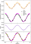 |
Fig. 5 Light curve taken at various facilities using the period 0. d 3347894. Upper panel: light curves of the CRTS survey, the PTF facility, WISE, and Gaia have absolute calibrations. Middle panel: TESS light curve cannot be calibrated absolutely (see text). Lower panel: all light curves normalized to the amplitude of unity. |
Journal of spectroscopic observations.
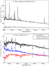 |
Fig. 6 Overview about the spectroscopic behaviour at different phases of the light curve. Upper panel: mean OSMOS spectra from 2021 February and March. The top trace is the average of spectra taken near maximum light, and the bottom trace near minimum light. The vertical axis is the same for both traces. Lower panel: upper, black trace shows the same minimum-light spectrum as the top trace. The red trace is a scaled spectrum of a K2 V star, while the blue trace resultsfrom subtracting the scaled K-type spectrum from the observed spectrum. |
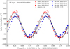 |
Fig. 7 Radial velocities of the absorption component and Hα emission line in YY Hya as a function of the period and epoch derived from the photometry. To preserve continuity, the data are repeated for one cycle. Solid lines show the best-fitting sinusoids. |
Radial velocities derived from emission and absorption lines.
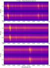 |
Fig. 8 Two-dimensional phase-resolved spectrum prepared as described in the text. The spectra used here are flux-calibrated. |
3 Proposed binary model
The photometric modulation and the time-resolved spectra show conclusively that YY Hya is a binary system in which a late-type star is strongly irradiated by a much hotter companion. This result, together with the UV excess, leads us to model the system as a compact binary system with a white dwarf (WD) causing the strong irradiation effects. Other than in the objects of the BE UMa family (see e.g., Shimansky et al. 2016), the WD is not luminous enough to contribute significantly, or even to dominate, the optical luminosity. The resulting WD, although providing more than 99.5% of the flux in the GALEX FUV band, contributes less than 1% in the optical evenduring minimum phase, when only the non-illuminated side of the K star is seen. The irradiation modelling here follows widely the methods and discussions in Hamilton-Drager et al. (2018) for the post–nova V723 Cas.
While the far side of the secondary star is near the state of the normal main-sequence star, the other side is strongly illuminated and heated. This causes the sinusoidal light curve. Such compact systems are normally in bound rotation (see e.g., Schandl et al. 1997). The recurrent nova CI Aql, even while shown to be a bit more massive and with a period of >0. d 6 a significantly larger system, behaves perfectly like this as well (Lederle & Kimeswenger 2003). Similar results are found by Haefner et al. (2004) and Parsons et al. (2010) in the case of the pre-cataclysmic variable NN Ser. The latter authors state that there is no detectable heating of the unirradiated face of the companion star, despite the fact that the intercepting radiative energy from the WD exceeds its luminosity by over a factor of 20.0. Assuming now a nearly constant temperature at the far side of the cold stellar component, together with the findings in the spectroscopy (Fig. 6), we obtained an initial guess for the system during minimum. The lack of an eclipse givesan upper boundary for the system inclination, which only marginally depends on the mass ratio, q.
As a hot compact companion does not suffer any deformation or irradiation effects and as is always visible, it can be modelled as constant contribution independent from the phase. This is especially important for the GALEX FUV band, wherethe large secondary star no longer contributes to the radiation, and thus no variation is expected at all.
Using the updated online version10 of the compilation and calibration by Pecaut & Mamajek (2013), we then obtained an upper limit of M* ≤ 0.8 M⊙ and a radius of R* ≈ 0.75 R⊙. The effective temperature then would be T*≤ 5000 K. This corresponds to the spectroscopy during minimum phase shown above. However, the 0.7–5 μm photometric colors during the minimum phase suggest a temperature that is likely nearer to 4000 K. This would correspond to a K6-7 star, with M*≈ 0.6 M⊙, R* ≥ 0.63 R⊙ and T* ≥ 4000 K. We attribute the difference to the fact that always a small fraction of the slightly heated transition zone towards the illuminated surface will show spectral lines resembling those of a slightly hotter star than that found in the near- and mid-infrared photometry. Due to the inclination of the system here, other than in the case of NN Ser, we always have some contamination from light from the hotter, illuminated side. This is supported by the distance estimate obtained from Gaia eDR3. The sole K2V star, without any additional illuminating effect, with the given magnitudes during minimum, would already lie at > 500 pc. However, the inclination always makes it so that there is some additional flux from the illuminated side contributing to the photometry even during minimum. This effect diminishes towards the red and infrared (see also the decomposition in Fig. 6).
The mass, MWD, of the compact companion and the ratio, q, is ultimately defined by the orbital period, P, the system inclination, i, and the velocity half amplitude, K, from our spectroscopy via the binary mass fraction
 (2)
(2)
where G is gravitational constant, resulting in 0.4 ≤ MWD ≤ 1.2 M⊙.
To model the light curve in detail we used the program Binary Maker 3 (BM3, Bradstreet & Steelman 2002)11. As mentioned already (and nicely shown in the case of the evolution of the post–nova V723 Cas moving ver the years to a low quiescence state), strong mass transfers and accretion discs cause significant asymmetric structures in the light curves (Hamilton-Drager et al. 2018). However, as we have a perfect sinusoidal light curve, we are able to assume a system without an accretion disk here for our model. As discussed in detail by Heber et al. (2018), the irradiation efficiency is not completely understood and thus a source of systematic uncertainty. Schaffenroth et al. (2019) used a large sample of spectroscopically investigated compact binary systems with hot subdwarf (sdB) companions, as part of the Eclipsing Reflection Effect Binaries from Optical Surveys (EREBOS) project, to show that the efficiency in such systems is near to complete absorption of the UV radiation by the secondary. Model atmospheres using the PHOENIX model atmosphere code for the M-type stars of the non-mass-transferring post-common-envelope binaries GD 245, NN Ser, AA Dor, and UU Sge show similar results (Barman et al. 2004). Thus, we adopted a unity value here.
A stochastic gradient descent method (Russell et al. 2010) led to various local solutions in the minimum χ2 search in the multidimensional parameter space. Therefore, we manually calculated a complete grid of light curves with inclinations varying for each mass within the above calculated range in steps of 1° and a variation of the mass 0.4 ≤ MWD ≤ 1.2 M⊙ in steps of 0.05 M⊙. The size, RMS, of the secondary was varied from ≈ 80% to exactly 100% of the Roche Lobe RRL in 12 steps. However, only within a few percent below the Roche Lobe perfect sinusoidal light curves were obtained. The temperatureof the compact companion was varied from 50 000 to 80 000 K. Then the luminosity of the compact star was adapted until the light curve amplitude in the TESS and the CRTS bands was recovered as observed at a phase interval of ± 0.05 around minimum and maximum (ϕMIN = 0.0 and ϕMAX = 0.5) each time. As the TESS photometric band is fairly red, this modelling does not suffer from the strong emission line regions at wavelengths below 5500 Å. As a next step, the goodness of the fit was calculated for the remaining phase regions via

The phase restriction for this calculation was used to avoid a dependency from the fit of the amplitude in the step before. A small sub-sample of the residuals (Idata − Imodel) of the light curves is shown in Fig. C.1. Purely based on the photometry, there is only one possible solution in inclination, i, for each temperature, TWD, and luminosity, LWD, for each of the selected MWD. Due to the nearly noise-free TESS light curve, this solution is very sensitive to the inclination i. Thus, around the preliminary solution, the grid was refined to 0.1 degree steps. The bandwidth of solutions varies only from 36 to just above 40° as function of the WD mass (Fig. 10). The system parameters, however, give us then a radial velocity. For an illuminated star, we have to expect that the emission lines originate only from the half of the star inwards to the mass center. Thus, the observed velocity half-maximum Kem∕sin(i) of the emission lines will underestimate the orbital velocity K from Eq. (2). On the other hand, the absorption lines originate from the weakly and unilluminated part, having its weighted center outside the mass center. Thus, the  from the absorption lines will be an overestimate. This is described also in detail for EC 11575-1845 and V664 Cas in Exter et al. (2005). We thus safely and very conservative may use those two extreme cases Kem∕sin(i) and
  as lower and upper boundaries, respectively. As indicated in Fig. 10, this limits the mass range for the white dwarf to 0.64< MWD < 0.85 M⊙, with a favorite mass of MWD ≈ 0.725 M⊙. The distance of the compact companion was then derived as well. The latter varies the luminosity in the mass-temperature plane (Fig. 11). However, the above mass constraints limit our further steps of the investigation to a small region in the luminosity-mass-temperature plane.
The luminosity LWD and the effective temperature TWD were a priori independent free parameters, but are linked to a single degree of freedom by the GALEX FUV flux and the known distance of the system. For this purpose, all WDs with T >50 000 K in the sample of Finley et al. (1997), where GALEX FUV measurements were available were used together with the new Gaia EDR3 distances to derive a relationship between those two parameters. For the GALEX photometry, the entire model grid from 50 000 <T < 150 000 K; 5.0 < log(g[cgs]) < 8.0 from Rauch (2003) was downloaded and folded with the published GALEX FUV filter curve (Rodrigo et al. 2013). However, as the dependency on gravity, log(g), is very small in our temperature range, this dimension was ultimately neglected. We used for the absolute calibration, the two hot WD stars 0004+330 (Teff = 85 000 K) and 0231+050 (Teff = 50 000 K) from the calibration sample for GALEX by Camarota & Holberg (2014) and the WD in NN Ser due to its very accurately known stellar radius (Haefner et al. 2004; Parsons et al. 2010). Although the statistical errors given for the GALEX data are very small, we used a conservative error estimate caused by a possible systematic error in the extinction correction AFUV of 50%. This leads us to the final temperature range TWD = 66 500 ± 3500 K (Fig. 12). The best model parameters are summarized in Table 3 and Fig. 13 shows the resulting geometry together with the light curve.
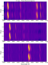 |
Fig. 9 Two-dimensional phase-resolved spectrum prepared as described in the text. The spectra used here are divided by the continuum. |
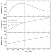 |
Fig. 10 Resulting best-fit model as function of the mass of the white dwarf. The inclination, i, of the system (top), the resulting K half velocityamplitude (middle), and the orbital separation of the mass centers of the stars (bottom panel). The dashed line marks the average between the extreme cases of the emission and the absorption line velocities, while the dotted lines mark the two extreme cases (see text). |
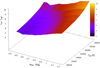 |
Fig. 11 Solution plane for the luminosity, LWD, as function of the mass and the effective temperature of the white dwarf for the complete model grid. The luminosity is color-coded as well for clarity. |
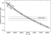 |
Fig. 12 Best model magnitude. The solution for the mass range defined from the velocities. The GALEX measurement error (dotted lines) are very small. Conservative estimates for systematic errors are indicated by the thick dashed lines. |
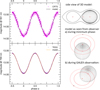 |
Fig. 13 BM3 model – best fit model based on the red passband TESS data and then calculated for the shorter wavelength CRTS data to constrain the temperatures of the components by the higher amplitude in the visual wavelength. The drawings (from top to bottom) show the side view including the Roche lobe limit, the model at minimum phase showing mainly the cold side of the MS star, and the phase during the GALEX observations showing nearly the whole hot side. The crosses mark the mass centers of the stars and the system barycenter. Red ellipses are the projected orbits. |
4 Galactic context
Together with our spectroscopy, the Gaia mission data allow us to derive a full 6D dynamical investigation of the source. Here, we used the Gaia EDR3 parallax and proper motions as well as the average of γ derived from the emission and the absorption lines as the system radial velocity, with a conservative error estimate due to the scatter in Fig. 7 (see Table 2). For the latter, we thus used vrad = 24 ± 10 km s−1. We used theGalactic potential as described by Allen & Santillan (1991) with the code of Odenkirchen & Brosche (1992) to compute the Galactic orbit and kinematic parameters of YY Hya analogously to the calculations in Pauli et al. (2006).
The orbit in the Cartesian Galactic coordinate frame X, Y, Z, with the Galactic center at theorigin and ρ parameterizing the Galactocentric distance (Fig. 14), is nearly circular and bound to the Galactic disk. Moreover, the comparison with the local WD sample by Pauli et al. (2006) also shows that the position of the radial versus the rotational velocity components and the angular component Jz perpendicular to the disk versus the orbital eccentricity e clearly puts YY Hya into the middle of the young thin disk population. The currently reached height Z = 155 pc above the disk plane is, in fact, close to the maximum elevation reached in orbit.
Consequently, we were able to use the metal-rich WD evolution tracks from the most recent calculations by Miller Bertolami (2016) for the WD component of YY Hya. The WD mass of 0.725 M⊙ gives us, based on the initial-to-final mass relation of Cummings et al. (2018), an initial stellar mass of 3–4 M⊙. As the progenitor thus was a late B-type star (Mowlavi et al. 2012; Eker et al. 2018; Serenelli et al. 2021) with a lifetime of approximately half a Gyr or slightly below that, we conclude that the K-star companion has barely evolved off the zero-age main sequence (ZAMS).
Parameters of the best-fit model.
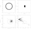 |
Fig. 14 Kinematics of YY Hya based on our spectroscopic system velocity and the Gaia parallax and proper motions. Upper panels: predicted orbit of YY Hya in the Milky Way for the next 2 Gyrs. Left: orbit projected on the Galactic plane, the Galactic center is at the origin. Right: meridional plot of the orbit. Lower panels: comparison of kinematic properties of YY Hya with the local WD sample by Pauli et al. (2006). Left: radial velocity component, U, versus the velocity, V, in rotational direction, the inner circle encloses the region of thin disk objects, the outer circle the thick disk regime. Right: angular momentum component, Jz, perpendicular to the plane versus the orbit eccentricity, e. |
5 Discussion and conclusion
From the data presented above, it is clear that YY Hya is not an RR Lyr star as classified up to now in the literature but is instead a compact binary of a late K-type main-sequence star with a hot WD companion. Due to a small separation, the system certainly went through a common envelope (CE) phase. The long term stability of the period and phase shown here, suggest that no major mass transfer is currently happening in this system. Moreover, the perfect symmetric and sinusoidal light curve supports that there is no accretion disk and no hot spot from an accretion stream.
Our spectroscopic results showing hardly any emission lines during minimum light phase means that its light curve is dominated by the irradiation of the compact hot WD on the secondary star. While the H and He emission lines are strongly broadened, other emission lines, mainly originating from the CNO group elements in low ionization states, are narrow. This is similar to the findings in the binaries of the BE UMa family formed mainly by EC 11575-1845 = TW CrV, V664 Cas = the central star of the planetary nebula HFG 1, HS 1857+5144, BE UMa, NN Ser = the central star of the PN ETHOS 1 = PN G068.1+11.0 (Exter et al. 2005; Aungwerojwit et al. 2007; Shimansky et al. 2009, 2008; Parsons et al. 2010; Mitrofanova et al. 2016; Munday et al. 2020).
BE UMa systems all exhibit sinusoidal light curves with no signatures of current mass transfer and active accretion. They also show spectra signatures of the white dwarf companion in the optical and have late M-type star companions (except BE UMa; Shimansky et al. 2008). The low-luminosity companions do not outshine the WD in the optical. Thus the emission line contrast over the continuum is much smaller. The contributing WD spectra with the wide strong H and He absorptions further reduce the emission line contrast for H and He lines. Thus all those effects we see in YY Hya are less pronounced there. But still we denote YY Hya as upper boundary case with higher mass companion within this class of BE UMa variables. UU Sge, the central star of the PN A63 (PN G053.8-03.0), also belonging to that class of objects, shows predominately much higher ionization levels for the CNO elements in the spectra (Wawrzyn et al. 2009). Older members of this physical family, with already much cooler WDs, might be MS Peg and LM Com (Shimansky et al. 2003). However, the low luminosity of the WDs in these systems result in much lower photometric amplitudes of 0m.1 to 0m.2 and only weak emission lines of neutral metals like Fe I, Na I, and Mg I.
Recently Kruckow et al. (2021) published a catalog from the literature containing more than 800 candidates of post-CE systems. Only the small fraction shown here belongs into our class of objects with periods below 1 day with no effects of the accretion of a cataclysmic variable yet. Indeed, these seem to form a class of post-CE but pre-cataclysmic variables. Investigations systematically searching for such close binary systems in the cores of PNe in the Gaia era will certainly expand the family (Chornay et al. 2021) but will be limited to the young objects of the group.
We follow the suggestion by Shimansky et al. (2016), who used the derived position along the temperature-time evolution of post-AGB white dwarfs to derive an age since the break of the AGB due to the CE phase. With the WD mass of  , we obtain an age since leaving the AGB of 520 to 600 kyr from the most recent evolutionary tracks by Miller Bertolami (2016). Shimansky et al. (2016) furthermore define the relative luminosity excess log (ΔL∕L) as the difference between the expected luminosity using a WD evolutionary track and the observed one in the HRD at the post-CE age of the system. The value of about −0.6 lies significantly above their relation. However, as the reanalysis of the central star of the PN ETHOS 1 shows, moving from the very old evolutionary tracks of Bloecker (1995) to the faster evolving modern post-AGB evolution change the system parameters already. Moreover, all systems there, except the very young and hot central star of PN ETHOS 1, have much lower WD masses. Thus the initial masses of the stars, forming the compact companion later, were much lower with the secondary stars being late M stars. The exception is BE UMa. However, that system is very wide (Porb =2. d 29).
The latter difference might be the main reason why YY Hya formed such a massive large nebula, while the young objects of the class all show nearly normal PNe. Two objects in the sample of Shimansky et al. (2016) with similar ages, namely EC 11575-1845 and HS 1857+5144, however, show similar spectroscopic and photometric signatures. Taking the size of the main nebula 4.8 pc and assuming a CE age of 520 to 600 kyr together with typical expansions of of 5 to 20 km s−1 for CE shells from models (Clayton et al. 2017; Glanz & Perets 2018), we end up in fact with a few hundred thousand years. Moreover, Clayton et al. (2017) show that the orbital effect pronounces episodic quasi-periodic mass-loss history during CE ejection. That will give a structured nebula as we see in the case of YY Hya.
To estimate a mass we used the Hα surface brightness using NEBULAR (Schirmer 2016). Assuming the shell being a aggregate of slabs with a thickness of 1% of the radius each, and assuming the brightest fragments cover about 10% along the line of sight in each case, we end up with a density nH of about 2 to 7 hydrogen atoms per cm3. Assuming that these fragments have a volume filling factor of few percent we end up with a shell of about one solar mass. This supports the idea that this nebula is the result of an ejected CE. Recombination time scales of such a plasma would be 25 000 to 100 000 years (Osterbrock & Ferland 2006). However, a static solution of the photoionization with the model of our WD and such a shell with CLOUDY (Ferland et al. 2017) leads to photoionization fractions of about 0.5 for the hydrogen. That, and the fact, that the WD was hotter and more luminous in recent history, slows down the recombination. The CLOUDY model also predict [O III](5007Å)/Hα line ratios of10−4. Thus we failed to observe the nebula in that line. Moreover, this model would predict a [O II](3726+29Å)/Hα of 0.3, promising for observations.
We carried out a multi-wavelength search, using the Aladin v11 image facilities (Bonnarel et al. 2000) from the radio (NVSS) over infrared (IRAS, AKARI, WISE, Planck), to X-rays (ROSAT) and γ-rays (Fermi). But neither the nebular center, nor the lobes appear in any of those images.
YY Hya’s high Galactic latitude and the absence of large interstellar clouds in its local vicinity, the geometry of the vis-à-vis lobes plus their enormous extent, makes the explanation of ionized interstellar matter very unlikely. Instead, they are likely termination bow shocks of jets formed during the CE phase. As the FUV flux is higher in these lobes than in the main nebula, the idea that they are termination shocks of a bipolar jet is supported by models (Chamandy et al. 2018)which show that the formation of such jets is not unusual for CE evolution. However, Chamandy et al. (2018) claim that the detailed physics near the cores still cannot be handled properly due to numerical limits on the large scale differences in the systems. Moreover, the direction defined by the lobes point toward the Galacticplane, which is located south-west of the target. there is a slight gradient of emission visible in the Planck and the AKARI images. The large distance of the lobes make a gradient of the ISM already likely on the target scale.This might be the reason why the south-west lobe is so much more prominent than the north-east one.
While the wide system of BD+46°442 (P > 140 days) certainly does not belong to this same class of CE objects, it currently shows such a jet formation (Bollen et al. 2017). Investigations of the young objects of the EB UMa class including UU Sge (Mitchell et al. 2007) and PN ETHOS 1 (Miszalski et al. 2011), as well as of PN G054.2-03.4 (The Necklace; Corradi et al. 2011) all show jet structures with a 3:1 size ratio compared to the main nebula. Moreover, Miszalski et al. (2011) find that all those structures are dynamically a few hundred years older than the main nebula. We note that in the case of YY Hya such a small offset will not be significant after such a long time of >500 kyr.
In summary, we find YY Hya to be a BE UMa type post-common enevelope pre-cataclysmic variable. Within this family of objects, the YY Hya system extends the upper limit of mass ranges found up to now, both for the primary as well as for the secondary star. A larger stellar shell is the reason for the massive large emission nebula and the far distant vis-à-vis lobes. Moreover, its high Galactic latitude (b = +20°) has helped to keep these structures largely undisturbed for a long time. Deep and high-resolution spectroscopy of these structures is encouraged to obtain insight into the spatio-kinematic structure as well as more detailed information on the excitation and recombination state of such shells.
Acknowledgements
We would like to thank the referee Steve Howell very much for his ideas for improving the original work. This research has made use of NASA’s Astrophysics Data System Bibliographic Services (ADS), use of the SVO Filter Profile Service supported from the Spanish MINECO through grant AYA2017-84089, NASA/IPAC Infrared Science Archive (IRSA), which is funded by the National Aeronautics and Space Administration and operated by the California Institute of Technology, and use of the SIMBAD database (Wenger et al. 2000), operated at CDS, Strasbourg, France. Furthermore this research made use of the Stellarium software (stellarium.org) version 0.19.1. and of the astrometry.net project, which is partially supported by the US National Science Foundation, the US National Aeronautics and Space Administration, and the Canadian National Science and Engineering Research Council. The CSS survey is funded by the National Aeronautics and Space Administration under Grant No. NNG05GF22G issued through the Science Mission Directorate Near-Earth Objects Observations Program. The CRTS survey is supported by the U.S. National Science Foundation under grants AST-0909182 and AST-1313422. This publication makes use of data products from the Wide-field Infrared Survey Explorer (WISE), which is a joint project of the University of California, Los Angeles, and the Jet Propulsion Laboratory/California Institute of Technology, funded by the National Aeronautics and Space Administration. The Intermediate Palomar Transient Factory (PTF) project is a scientific collaboration among the California Institute of Technology, Los Alamos National Laboratory, the University of Wisconsin, Milwaukee, the Oskar Klein Center, the Weizmann Institute of Science, the TANGO Program of the University System of Taiwan, and the Kavli Institute for the Physics and Mathematics of the Universe. The MDM Observatory is operated by Dartmouth College, Columbia University, Ohio State University, Ohio University, and the University of Michigan. This work presents results from the European Space Agency (ESA) space mission Gaia. Gaia data are being processed by the Gaia Data Processing and Analysis Consortium (DPAC). Funding for the DPAC is provided by national institutions, in particular the institutions participating in the Gaia MultiLateral Agreement (MLA). The Gaia mission website is https://www.cosmos.esa.int/gaia. The Galaxy Evolution Explorer (GALEX) is a NASA Small Explorer. We gratefully acknowledge NASA’s support for construction, operation, and science analysis for the GALEX mission, developed in cooperation with the Centre National d’Etudes Spatiales of France and the Korean Ministry of Science and Technology. This paper includes data collected by the TESS mission. Funding for the TESS mission is provided by the NASA Explorer Program.
Appendix A Photometry data
In Table A.1, we provide a summary for the observations for the time series used in this paper. Table A.2 gives an overview of the photometry. The passbands and zero points are taken from the continuously maintained online data base12 of the SVO filter service(Rodrigo et al. 2013). In the case of Gaia, where several filter sets are defined for DR2, we used the revised definition by Weiler (2018) from the data base. The interstellar extinction calculation is based on Cardelli et al. (1989) and the adopted reddening value of E(B − V) = 0.m032 using R = 3.1. As the line of sight is far from the Galactic plane and does not show major dense clouds in the vicinity, these values derived for the thin interstellar matter seem to be most applicable. Due to the small value of the extinction, in fact, the selection of the curve type and of R does not cause a significant variation of the result. For those data sets, where a full fit of the light curve was possible, the minimum, mean, and maximum from the derived sinusoidal curve fit is used. For the experiments and bands where only one or two measurements were given the phase of the measurement is given together with the magnitude,  . Furthermore, we used the wavelength–magnitude relation from the large data time series to calculate anestimate for the minimum brightness and corrected for interstellar extinction leading to
  . Only for the GALEX data no such amplitude correction was derived. As discussed earlier in this work, we do not have to assume a significant amplitude for the far-UV component.
Time span, passband definition, and number of available data points for the photometric observations.
Overview of the photometric bands, used effective wavelengths, λeff, calibration zero points, ZP, and the interstellar extinction, Aλ. In addition, an overview of the magnitudes as used in the SED fitting (see text) is given.
Appendix B Narrow-band image calibration
The image mosaic was obtained from 294 images taken at the CHILESCOPE facilities. CHILESCOPE13 is a remotely controlled commercial observatory located in the Chilean Andes (70°45′53′′ W, 30°28′15′′ S, 1567 m a.s.l.) about 25 km south of the Gemini South and LSST telescope site Cerro Pachón. We used the two 50cm Newtonian telescopes built by Astro System Austria (ASA)14. These telescopes have a focal ratio f/3.8 and are equipped with 4 K × 4 K FLI PROLINE 1680315 CCD cameras, yielding a pixel scale of 0′′.963 pixel−1 and a FOV of 1°.096 × 1°.096. Furthermore, we used, for the mosaic, the Hα (FWHM 3nm) filter from Astrodon16. This filter is know to suppress contamination from possible [N II] to a level below 5% of the intensity of those lines. As the [N II]:[S II] ratio is about 10:1 in shocked nebulae such as supernovae remnants and even lower for H II regions (Magrini et al. 2003; Barría et al. 2018); and as [S II] was not detected in even the brightest regions, we are able to conclude that we do not suffer from contamination by the nitrogen line.
Each individual exposure time was 20 minutes around 9 pointing positions with their FOV overlapping 50% each. A total exposure time of about 100 hours was accumulated. Due to the overlap, the central regions were covered with a total exposure time of 40 hours, while the outer ring with 25% of the image width was covered only by 20 hours. However, the very corners were mapped for only about 11 hours. To compensate for minor variations due to weather, seeing, and airmass, in the overlapping regions, a common set of about 300 stars ranging from a 5σ detection level until the overexposure at the central pixels were extracted using SExtractor v 2.19.5 (2019-07-27) (Bertin & Arnouts 1996). They were used to scale the frames to a common flux calibration. The median of this calibration was used and the root mean square (rms) of these calibration factor was about 20%. The worst case was a set of less than ten frames, achieving only about 50% of the median flux. Due to the high overlap of up to 120 fields, no special noise suppression handling for those fields after the flux scaling was required.
The astrometry was obtained by the use of a local installation of solve-field and wcs-resample of the astrometry.net17 suite v0.85 (Lang et al. 2010) with a Gaia eDR3 catalog subset of the surrounding 3° field. To get a proper distortion correction ofthis fast f/3.8 telescopes a 4th order projection correction prior to stacking the images was required. The final positional rms was below 1/5th of a pixel. Resampling to this grid allowed us to generate a mean image. Then, for each position, the image count varies from 32 to 120 frames. We used the mean value of the pixels, eliminating the three lowest and three highest values. This removed the cosmics and satellite spurs, but still reduced noise by building means for a large number of frames. Thus, this approach is superior to simply using the median value.
Lacking calibrator and standard fields in the used Hα filter set, Gaia data were used to derive an absolute flux estimation. About 1000 stars from the central region just outside of the main nebulaand from the NE and the SW corner field were matched with Gaia eDR3 stars. The red band magnitudes Gaia RP and the BP − BR color were used to derive the zero point ZP and a linear color term:

While the rms of the ZP for the stars mGaia RP < 17m.5 was better than 0m.02 only minor systematic variations of the order of 0m.08 were found between the better covered central region and the extreme field corners (Fig. B.1). The color term kλ = 0m.35 ± 0m.11 was derived. To derive a flux calibration of the emission line, the stellar flux f had to be integrated over the response curve I of the 3 nm wide filter:
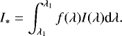
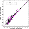 |
Fig. B.1 Magnitude calibration near the field center (black) and the extreme north east corner (magenta). The Gaia catalog limited the faint end, while the CHILESCOPE Hα goes about 1.m5 deeper. |
As the colors of the field stars show that the sample is dominated by stars later than G5, we can assume that the Hα absorption lines do not dominate the flux variation in that region and the stars in a statistical average and we thus can take out the f(λ) from the integral in this small wavelength region. The response curve I(λ) of the Astrodon filters published by the vendor was integrated numerically, giving a value of 2.95 nm. The monocromatic flux in the Vega system was obtained again from the SVO filter service (Rodrigo et al. 2013) from various published 3 nm Hα filters from ING, ESO, and TNG. They vary by less that 4%. We thus adopted for mH α = 0m.0 the mean value off(λ) = 1.65 10−9 erg cm−2 s−1Å−1. Using this calibration, we obtained a zero point for the surface brightness of 2.8 10−17 erg cm−2 s−1 arcsec−1 for the mosaic.
Observed emission lines in YY Hya at phase 0.5. Listed line strengths are relative to C III λ4650 = 100.
Appendix C Model grid
Figure C.1 shows a fraction of the whole grid of models. The effects of the most critical parameters for the modeling, namely, the system inclination, i, and the fraction of the donor star radius in units of the Roche lobe radius, RRoche, are demonstrated for the solution fulfilling the best match to the amplitude for this pair of parameters.
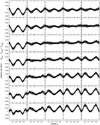 |
Fig. C.1 Section of the model grid for lowest mass of the grid (MWD = 0.4M⊙). The deviation of the TESS data intensity Idata to the model Imodel as function of the phase is shown. The columns are for constant radius of the donor star (from left to right) are: 1.000, 0.955, 0.910, 0.865, and 0.820 times of the Roche lobe radius, RRoche. Along the rows, the system inclination, i, varies from 28° to 52° in steps of 4°. The compact companion luminosity was varied each time to fit the system amplitude (see Sect. 3). |
Appendix D Possible Historical Link
Finally, albiet a bit speculative, we briefly discuss a possible link of YY Hya and its nebula with an apparent “guest star” sighting in Hydra reported in August and September 1065 AD by Korean and Chinese astronomers (Hsi 1957; Ho 1962; Kronk 1999). Although the secondary is not Roche Lobe filling and thus is not yet feeding accretion, fallback from the very slowly ejected CE envelope may cause possibly similar accretion at slower scales on the WD. Taking into account the rotation of the equinox, we find YY Hya to lie at α =08h43m26s, δ = −18°25′54′′ in 1065 AD.Assuming an observational site in China where the location of YY Hya was visible above the horizon,then YY Hya would be visible about 1.5 hours before sunrise and reach a position about 14° above the horizon at the end of the night. It would appear just above the constellation called the celestial temple in the medieval Chinese constellation map by Su Song dated 1092 (Needham 1959). Using this position and constellations as input to Stellarium18, we find thatthe YY Hya is near to the constellation Tian Miao ( – also called Tiān Miào, Tiānmiào, Thien-miao and T’ien-Miao) containing 14 stars. The precession-corrected position of YY Hya is indicated as well (Fig. D.1). That is what (Hsi 1957) mentions for the vicinity of the 1065 event. Furthermore, it corresponds to the maps in the investigation about ancient comets in Williams (1871) and independently in the framework of the tail of the comet of 1385 in Hind (1845). They appoint this region mostly covered nowadays by Pyxis (or Pixis Nautica).
 |
Fig. D.1 Visibility of the region of YY Hya in the morning hours of September, 11 1065 from Beijing, China using medieval Chinese constellations. Circle marks the position of YY Hya. The plot was generated by Stellarium 0.19.1 |
The position of YY Hya is just on the border to this modern constellation definition19. Moreover, the crude positional estimate of α = 10h20m, δ = −30° in B1950 (α = 09h49m, δ = −25°30′ in 1065) given by Hsi (1957) (which is, in fact, near to the mV = 4m.25 star α Ant) was too much south and not observable in nighttime from China at that time. Thus, we decided not to further consider this result. In view of these positional agreements, we propose that the link of the 1065 AD transient event with YY Hya is at least possible.
Assuming a typical absolute visual magnitude of a Nova with MV ≈−8m.0, it should have been at mV ≈ +0m.2. As there are no stars brighter than mV < +4m.0 in roughly 13°.5 from the position, and the nearest planet was Saturn at a distance of over 25 degrees away in late August and September 1065 AD, it would seem the 1065 AD guest star may have been fairly noticeable given this nearly empty bright star region of the sky. However, with an angular size of 36′ (≡ 4.8 pc @ DGaia = 456 pc) and an age of about 1000 years, YY Hya’s main nebula would require an average expansion of slightly above 2200 km s−1 if it was created in a single event. The outer lobes lying at a distance of 11.5 pc would lead to jets with even higher velocities, around 11 200 km s−1. These are details that we do not observe in this case. Also, the mass estimate of the shell is by several orders of magnitudes too large for a single Nova event. Thus, this excludes the possibility that the nebulae around YY Hya was generated during the aforementioned event some 1000 years ago.
References
- Allen, C., & Santillan, A. 1991, Rev. Mex. Astron. Astrofis., 22, 255 [NASA ADS] [Google Scholar]
- Aungwerojwit, A., Gänsicke, B. T., Rodríguez-Gil, P., et al. 2007, A&A, 469, 297 [NASA ADS] [CrossRef] [EDP Sciences] [Google Scholar]
- Barman, T. S., Hauschildt, P. H., & Allard, F. 2004, ApJ, 614, 338 [Google Scholar]
- Barría, D., Kimeswenger, S., Kausch, W., & Goldman, D. S. 2018, A&A, 620, A84 [NASA ADS] [CrossRef] [EDP Sciences] [Google Scholar]
- Bertin, E., & Arnouts, S. 1996, A&AS, 117, 393 [NASA ADS] [CrossRef] [EDP Sciences] [Google Scholar]
- Bianchi, L. 1999, Mem. Soc. Astron. It., 70, 365 [Google Scholar]
- Bianchi, L., Herald, J., Efremova, B., et al. 2012, VizieR Online Data Catalog: II/312 [Google Scholar]
- Bloecker, T. 1995, A&A, 297, 727 [Google Scholar]
- Bollen, D., Van Winckel, H., & Kamath, D. 2017, A&A, 607, A60 [NASA ADS] [CrossRef] [EDP Sciences] [Google Scholar]
- Bonnarel, F., Fernique, P., Bienaymé, O., et al. 2000, A&AS, 143, 33 [NASA ADS] [CrossRef] [EDP Sciences] [Google Scholar]
- Boyce, E. H. 1936, Harvard College Observ. Bull., 903, 28 [Google Scholar]
- Bradstreet, D. H., & Steelman, D. P. 2002, AAS Meeting Abstracts, 201, 75.02 [NASA ADS] [Google Scholar]
- Camarota, L., & Holberg, J. B. 2014, MNRAS, 438, 3111 [NASA ADS] [CrossRef] [Google Scholar]
- Cardelli, J. A., Clayton, G. C., & Mathis, J. S. 1989, ApJ, 345, 245 [Google Scholar]
- Castelli, F., & Kurucz, R. L. 2003, IAU Symp., 210, A20 [Google Scholar]
- Catelan, M., Pritzl, B. J., & Smith, H. A. 2004, ApJS, 154, 633 [Google Scholar]
- Chamandy, L., Frank, A., Blackman, E. G., et al. 2018, MNRAS, 480, 1898 [NASA ADS] [CrossRef] [Google Scholar]
- Chornay, N., Walton, N. A., Jones, D., et al. 2021, A&A, 648, A95 [NASA ADS] [CrossRef] [EDP Sciences] [Google Scholar]
- Clayton, M., Podsiadlowski, P., Ivanova, N., & Justham, S. 2017, MNRAS, 470, 1788 [NASA ADS] [CrossRef] [Google Scholar]
- Corradi, R. L. M., Sabin, L., Miszalski, B., et al. 2011, MNRAS, 410, 1349 [CrossRef] [Google Scholar]
- Cummings, J. D., Kalirai, J. S., Tremblay, P. E., Ramirez-Ruiz, E., & Choi, J. 2018, ApJ, 866, 21 [NASA ADS] [CrossRef] [Google Scholar]
- Dambis, A. K., Berdnikov, L. N., Kniazev, A. Y., et al. 2013, MNRAS, 435, 3206 [Google Scholar]
- Drake, A. J., Djorgovski, S. G., Mahabal, A., et al. 2009, ApJ, 696, 870 [Google Scholar]
- Drake, A. J., Djorgovski, S. G., Catelan, M., et al. 2017, MNRAS, 469, 3688 [NASA ADS] [CrossRef] [Google Scholar]
- Eker, Z., Bak"i"ş, V., Bilir, S., et al. 2018, MNRAS, 479, 5491 [NASA ADS] [CrossRef] [Google Scholar]
- Epchtein, N., de Batz, B., Capoani, L., et al. 1997, The Messenger, 87, 27 [NASA ADS] [Google Scholar]
- Exter, K. M., Pollacco, D. L., Maxted, P. F. L., Napiwotzki, R., & Bell, S. A. 2005, MNRAS, 359, 315 [Google Scholar]
- Feinstein, A. D., Montet, B. T., Foreman-Mackey, D., et al. 2019, PASP, 131, 094502 [Google Scholar]
- Ferland, G. J., Chatzikos, M., Guzmán, F., et al. 2017, Rev. Mexicana Astron. Astrofis., 53, 385 [Google Scholar]
- Finley, D. S., Koester, D., & Basri, G. 1997, ApJ, 488, 375 [NASA ADS] [CrossRef] [Google Scholar]
- Gaia Collaboration (Brown, A. G. A., et al.) 2018, A&A, 616, A1 [NASA ADS] [CrossRef] [EDP Sciences] [Google Scholar]
- Gaia Collaboration (Brown, A. G. A., et al.) 2021, A&A, 649, A1 [NASA ADS] [CrossRef] [EDP Sciences] [Google Scholar]
- Gao, X.-H. 2016, Res. Astron. Astrophys., 16, 184 [Google Scholar]
- Glanz, H. & Perets, H. B. 2018, MNRAS, 478, L12 [NASA ADS] [CrossRef] [Google Scholar]
- Green, G. M., Schlafly, E., Zucker, C., Speagle, J. S., & Finkbeiner, D. 2019, ApJ, 887, 93 [NASA ADS] [CrossRef] [Google Scholar]
- Guthnick, P., & Prager, R. 1936, Astron. Nachr., 260, 393 [NASA ADS] [CrossRef] [Google Scholar]
- Haefner, R., Fiedler, A., Butler, K., & Barwig, H. 2004, A&A, 428, 181 [NASA ADS] [CrossRef] [EDP Sciences] [Google Scholar]
- Hambly, N. C., MacGillivray, H. T., Read, M. A., et al. 2001, MNRAS, 326, 1279 [NASA ADS] [CrossRef] [Google Scholar]
- Hamilton-Drager, C. M., Lane, R. I., Recine, K. A., et al. 2018, AJ, 155, 58 [NASA ADS] [CrossRef] [Google Scholar]
- Heber, U., Irrgang, A., & Schaffenroth, J. 2018, Open Astron., 27, 35 [Google Scholar]
- Hind, J. 1845, Lond. Edinb. Dubl. Phil. Mag. J. Sci., 27, 416 [Google Scholar]
- Ho, P. Y. 1962, Vistas Astron., 5, 127 [NASA ADS] [CrossRef] [Google Scholar]
- Hoadley, K., Martin, D. C., Metzger, B. D., et al. 2020, Nature, 587, 387 [NASA ADS] [CrossRef] [Google Scholar]
- Holl, B., Audard, M., Nienartowicz, K., et al. 2018, A&A, 618, A30 [NASA ADS] [CrossRef] [EDP Sciences] [Google Scholar]
- Hsi, T.-T. 1957, Smith. Contrib. Astrophys., 2, 109 [NASA ADS] [Google Scholar]
- Keenan, P. C., & McNeil, R. C. 1989, ApJS, 71, 245 [Google Scholar]
- Knigge, C., Baraffe, I., & Patterson, J. 2011, ApJS, 194, 28 [Google Scholar]
- Kronk, G. W. 1999, Cometography: A Catalog of Comets (Cambridge University Press), 1, 1799 [NASA ADS] [Google Scholar]
- Kruckow, M. U., Neunteufel, P. G., Di Stefano, R., Gao, Y., & Kobayashi, C. 2021, arXiv e-prints, [arXiv:2107.05221] [Google Scholar]
- Lallement, R., Babusiaux, C., Vergely, J. L., et al. 2019, A&A, 625, A135 [NASA ADS] [CrossRef] [EDP Sciences] [Google Scholar]
- Lang, D., Hogg, D. W., Mierle, K., Blanton, M., & Roweis, S. 2010, AJ, 139, 1782 [Google Scholar]
- Law, N. M., Kulkarni, S. R., Dekany, R. G., et al. 2009, PASP, 121, 1395 [NASA ADS] [CrossRef] [Google Scholar]
- Lederle, C., & Kimeswenger, S. 2003, A&A, 397, 951 [NASA ADS] [CrossRef] [EDP Sciences] [Google Scholar]
- Magrini, L., Perinotto, M., Corradi, R. L. M., & Mampaso, A. 2003, A&A, 400, 511 [NASA ADS] [CrossRef] [EDP Sciences] [Google Scholar]
- Martin, D. C., Fanson, J., Schiminovich, D., et al. 2005, ApJ, 619, L1 [Google Scholar]
- Martini, P., Stoll, R., Derwent, M. A., et al. 2011, PASP, 123, 187 [NASA ADS] [CrossRef] [Google Scholar]
- Miller Bertolami, M. M. 2016, A&A, 588, A25 [NASA ADS] [CrossRef] [EDP Sciences] [Google Scholar]
- Miszalski, B., Corradi, R. L. M., Boffin, H. M. J., et al. 2011, MNRAS, 413, 1264 [NASA ADS] [CrossRef] [Google Scholar]
- Mitchell, D. L., Pollacco, D., O’Brien, T. J., et al. 2007, MNRAS, 374, 1404 [NASA ADS] [CrossRef] [Google Scholar]
- Mitrofanova, A. A., Shimansky, V. V., Borisov, N. V., Spiridonova, O. I., & Gabdeev, M. M. 2016, Astron. Rep., 60, 252 [NASA ADS] [CrossRef] [Google Scholar]
- Morgan, D. 1995, IEEE Spectrum, 6, 25 [NASA ADS] [Google Scholar]
- Mowlavi, N., Eggenberger, P., Meynet, G., et al. 2012, A&A, 541, A41 [NASA ADS] [CrossRef] [EDP Sciences] [Google Scholar]
- Munday, J., Jones, D., García-Rojas, J., et al. 2020, MNRAS, 498, 6005 [Google Scholar]
- Needham, J. 1959, Science and Civilisation in China, Mathematics and the Sciences of the Heavens and the Earth (Cambridge: Cambridge University Press), 3 [Google Scholar]
- Odenkirchen, M., & Brosche, P. 1992, Astron. Nachr., 313, 69 [NASA ADS] [CrossRef] [Google Scholar]
- Osterbrock, D. E. & Ferland, G. J. 2006, Astrophysics of gaseous nebulae and active galactic nuclei, 2nd Ed. (University Science Books: Sausalito, CA) [Google Scholar]
- Parker, Q. A., Bojičić, I. S., & Frew, D. J. 2016, J. Phys. Conf. Ser., 728, 032008 [NASA ADS] [CrossRef] [Google Scholar]
- Parker, Q. A., Bojičić, I., & Frew, D. J. 2017, IAU Symp., 323, 36 [NASA ADS] [Google Scholar]
- Parsons, S. G., Marsh, T. R., Copperwheat, C. M., et al. 2010, MNRAS, 402, 2591 [Google Scholar]
- Patterson, J., Stone, G., Kemp, J., et al. 2018, PASP, 130, 064202 [NASA ADS] [CrossRef] [Google Scholar]
- Pauli, E. M., Napiwotzki, R., Heber, U., Altmann, M., & Odenkirchen, M. 2006, A&A, 447, 173 [NASA ADS] [CrossRef] [EDP Sciences] [Google Scholar]
- Pecaut, M. J., & Mamajek, E. E. 2013, ApJS, 208, 9 [Google Scholar]
- Rauch, T. 2003, A&A, 403, 709 [NASA ADS] [CrossRef] [EDP Sciences] [Google Scholar]
- Ricker, G. R., Winn, J. N., Vanderspek, R., et al. 2015, J. Astron. Teles. Instrum. Syst., 1, 014003 [Google Scholar]
- Rodrigo, C., Solano, E., & Bayo, A. 2013, SVO Filter Profile Service Version 1.0, IVOA Note 10 May 2013 [Google Scholar]
- Russell, S., Russell, S., Norvig, P., & Davis, E. 2010, Artificial Intelligence: A Modern Approach, Prentice Hall series in artificial intelligence (USA: Prentice Hall) [Google Scholar]
- Schaffenroth, V., Barlow, B. N., Geier, S., et al. 2019, A&A, 630, A80 [NASA ADS] [CrossRef] [EDP Sciences] [Google Scholar]
- Schandl, S., Meyer-Hofmeister, E., & Meyer, F. 1997, A&A, 318, 73 [NASA ADS] [Google Scholar]
- Schirmer, M. 2016, PASP, 128, 114001 [NASA ADS] [CrossRef] [Google Scholar]
- Schneider, D. P., & Young, P. 1980, ApJ, 238, 946 [NASA ADS] [CrossRef] [Google Scholar]
- Serenelli, A., Weiss, A., Aerts, C., et al. 2021, A&ARv, 29, 4 [Google Scholar]
- Shimansky, V. V., Borisov, N. V., Pozdnyakova, S. A., et al. 2008, Astron. Rep., 52, 558 [NASA ADS] [CrossRef] [Google Scholar]
- Shimansky, V. V., Borisov, N. V., & Shimanskaya, N. N. 2003, Astronomy Reports, 47, 763 [NASA ADS] [CrossRef] [Google Scholar]
- Shimansky, V. V., Pozdnyakova, S. A., Borisov, N. V., et al. 2009, Astrophys. Bull., 64, 349 [NASA ADS] [CrossRef] [Google Scholar]
- Shimansky, V. V., Mitrofanova, A. A., Borisov, N. V., Fabrika, S. N., & Galeev, A. I. 2016, Astrophys. Bull., 71, 463 [NASA ADS] [CrossRef] [Google Scholar]
- Skrutskie, M. F., Schneider, S. E., Stiening, R., et al. 1997, Astrophys. Space Sci. Lib., 210 25 [NASA ADS] [CrossRef] [Google Scholar]
- Stellingwerf, R. F. 1978, ApJ, 224, 953 [Google Scholar]
- Tonry, J., & Davis, M. 1979, AJ, 84, 1511 [Google Scholar]
- Wawrzyn, A. C., Barman, T. S., Günther, H. M., Hauschildt, P. H., & Exter, K. M. 2009, A&A, 505, 227 [NASA ADS] [CrossRef] [EDP Sciences] [Google Scholar]
- Weiler, M. 2018, A&A, 617, A138 [NASA ADS] [CrossRef] [EDP Sciences] [Google Scholar]
- Wenger, M., Ochsenbein, F., Egret, D., et al. 2000, A&AS, 143, 9 [NASA ADS] [CrossRef] [EDP Sciences] [Google Scholar]
- West, R. M. 1974, S&T, 48, 224 [NASA ADS] [Google Scholar]
- Williams, J. 1871, MNRAS, 32, 32 [NASA ADS] [CrossRef] [Google Scholar]
Serra Alta, Brazil: 53°.0426 W, 26°.7285 S.
All Tables
Time span, passband definition, and number of available data points for the photometric observations.
Overview of the photometric bands, used effective wavelengths, λeff, calibration zero points, ZP, and the interstellar extinction, Aλ. In addition, an overview of the magnitudes as used in the SED fitting (see text) is given.
Observed emission lines in YY Hya at phase 0.5. Listed line strengths are relative to C III λ4650 = 100.
All Figures
|
Fig. 1 Hα image taken at Serra Alta, Brazil of the region around YY Hya. Left: original image. Right: image following the star removal procedure (see text). The inner main nebula has a diameter of 36′. In the northeast and southwest corners, the vis-à-vis emission structures are clearly visible, both 47′ from the variable star. Northeast structure is just at the image edge and partly cut off. |
| In the text | |
|
Fig. 2 Hα image mosaic obtained at CHILESCOPE with a linear gray-scale mapping with surface brightness from zero to 1.5 10−16 erg cm−2 s−1 arcsec−1. The stellar limiting magnitude is about Gaia RP ≈ 21m. 8. The round nebula southwards is not related to our target but the beforehand known planetary nebula StDr 47 (PN G253.7+19.4, 09h27m31s. 46, −23°22′34″.40). |
| In the text | |
|
Fig. 3 MDM Hα images of the northeastern (left) and southwestern (right) outlying nebulosities around YY Hya showing the presence of emissions of overlapping shocks. |
| In the text | |
|
Fig. 4 GALEX FUV (left) and GALEX NUV (right) composite mosaic image. The 36′ circle and the two 47′ arcs are centered with respect to the position of YY Hya. While the central nebula is not clearly detected, the two vis-à-vis emission lobes are clearly visible in both bands. |
| In the text | |
|
Fig. 5 Light curve taken at various facilities using the period 0. d 3347894. Upper panel: light curves of the CRTS survey, the PTF facility, WISE, and Gaia have absolute calibrations. Middle panel: TESS light curve cannot be calibrated absolutely (see text). Lower panel: all light curves normalized to the amplitude of unity. |
| In the text | |
|
Fig. 6 Overview about the spectroscopic behaviour at different phases of the light curve. Upper panel: mean OSMOS spectra from 2021 February and March. The top trace is the average of spectra taken near maximum light, and the bottom trace near minimum light. The vertical axis is the same for both traces. Lower panel: upper, black trace shows the same minimum-light spectrum as the top trace. The red trace is a scaled spectrum of a K2 V star, while the blue trace resultsfrom subtracting the scaled K-type spectrum from the observed spectrum. |
| In the text | |
|
Fig. 7 Radial velocities of the absorption component and Hα emission line in YY Hya as a function of the period and epoch derived from the photometry. To preserve continuity, the data are repeated for one cycle. Solid lines show the best-fitting sinusoids. |
| In the text | |
|
Fig. 8 Two-dimensional phase-resolved spectrum prepared as described in the text. The spectra used here are flux-calibrated. |
| In the text | |
|
Fig. 9 Two-dimensional phase-resolved spectrum prepared as described in the text. The spectra used here are divided by the continuum. |
| In the text | |
|
Fig. 10 Resulting best-fit model as function of the mass of the white dwarf. The inclination, i, of the system (top), the resulting K half velocityamplitude (middle), and the orbital separation of the mass centers of the stars (bottom panel). The dashed line marks the average between the extreme cases of the emission and the absorption line velocities, while the dotted lines mark the two extreme cases (see text). |
| In the text | |
|
Fig. 11 Solution plane for the luminosity, LWD, as function of the mass and the effective temperature of the white dwarf for the complete model grid. The luminosity is color-coded as well for clarity. |
| In the text | |
|
Fig. 12 Best model magnitude. The solution for the mass range defined from the velocities. The GALEX measurement error (dotted lines) are very small. Conservative estimates for systematic errors are indicated by the thick dashed lines. |
| In the text | |
|
Fig. 13 BM3 model – best fit model based on the red passband TESS data and then calculated for the shorter wavelength CRTS data to constrain the temperatures of the components by the higher amplitude in the visual wavelength. The drawings (from top to bottom) show the side view including the Roche lobe limit, the model at minimum phase showing mainly the cold side of the MS star, and the phase during the GALEX observations showing nearly the whole hot side. The crosses mark the mass centers of the stars and the system barycenter. Red ellipses are the projected orbits. |
| In the text | |
|
Fig. 14 Kinematics of YY Hya based on our spectroscopic system velocity and the Gaia parallax and proper motions. Upper panels: predicted orbit of YY Hya in the Milky Way for the next 2 Gyrs. Left: orbit projected on the Galactic plane, the Galactic center is at the origin. Right: meridional plot of the orbit. Lower panels: comparison of kinematic properties of YY Hya with the local WD sample by Pauli et al. (2006). Left: radial velocity component, U, versus the velocity, V, in rotational direction, the inner circle encloses the region of thin disk objects, the outer circle the thick disk regime. Right: angular momentum component, Jz, perpendicular to the plane versus the orbit eccentricity, e. |
| In the text | |
|
Fig. B.1 Magnitude calibration near the field center (black) and the extreme north east corner (magenta). The Gaia catalog limited the faint end, while the CHILESCOPE Hα goes about 1.m5 deeper. |
| In the text | |
|
Fig. C.1 Section of the model grid for lowest mass of the grid (MWD = 0.4M⊙). The deviation of the TESS data intensity Idata to the model Imodel as function of the phase is shown. The columns are for constant radius of the donor star (from left to right) are: 1.000, 0.955, 0.910, 0.865, and 0.820 times of the Roche lobe radius, RRoche. Along the rows, the system inclination, i, varies from 28° to 52° in steps of 4°. The compact companion luminosity was varied each time to fit the system amplitude (see Sect. 3). |
| In the text | |
|
Fig. D.1 Visibility of the region of YY Hya in the morning hours of September, 11 1065 from Beijing, China using medieval Chinese constellations. Circle marks the position of YY Hya. The plot was generated by Stellarium 0.19.1 |
| In the text | |
Current usage metrics show cumulative count of Article Views (full-text article views including HTML views, PDF and ePub downloads, according to the available data) and Abstracts Views on Vision4Press platform.
Data correspond to usage on the plateform after 2015. The current usage metrics is available 48-96 hours after online publication and is updated daily on week days.
Initial download of the metrics may take a while.