| Issue |
A&A
Volume 655, November 2021
|
|
|---|---|---|
| Article Number | A50 | |
| Number of page(s) | 7 | |
| Section | Planets and planetary systems | |
| DOI | https://doi.org/10.1051/0004-6361/202141582 | |
| Published online | 19 November 2021 | |
Drag forces on porous aggregates in protoplanetary disks
Faculty of Physics, University of Duisburg-Essen,
Lotharstr. 1,
47057
Duisburg,
Germany
e-mail: This email address is being protected from spambots. You need JavaScript enabled to view it.
Received:
18
June
2021
Accepted:
23
September
2021
Abstract
Context. In protoplanetary disks, particle–gas interactions are a key part of the early stages of pre-planetary evolution. As dust particles grow into porous aggregates, treating drag forces of aggregates in the same way as those of monolithic compact spheres has always been an approximation.
Aims. The substructures and building blocks of aggregates may respond differently to different drag regimes than the overall size of the porous body would suggest. The influence of porosity and substructure size on the drag on porous bodies is studied.
Methods. We measured centimeter-sized porous aggregates with volume filling factors as low as ~10−4 for the first time in low-pressure wind tunnel experiments. Various substructures of different sizes down to micrometer (μm) resolution are tested. Knudsen numbers for the centimeter-sized superstructure are between 0.005 and 0.1 and Reynolds numbers are between 5 and 130.
Results. We find that bodies are subject to increasingly large drag forces with increasing porosity, significantly larger than previously thought. In the parameter range measured, drag can increase by a factor of 23, and extrapolation suggests even larger values. We give an empirically determined model for an adjusted drag force.
Conclusions. Our findings imply that the coupling of highly porous bodies in protoplanetary disks is significantly stronger than assumed in previous works. This decreases collision velocities and radial drift speeds and might allow porous bodies to grow larger under certain conditions before they become compacted.
Key words: protoplanetary disks / planets and satellites: formation
© ESO 2021
1 Introduction
Planet formation in protoplanetary disks involves particle growth of many orders of magnitude. One major element for particle motion is its interaction with the gas of the disk. Gas drag sets the sedimentation speed of dust toward the midplane (Dullemond & Dominik 2004; Riols & Lesur 2018) and is responsible for inward drift and the radial-drift barrier (Weidenschilling 1977; Demirci et al. 2019; Misener et al. 2019; Bogdan et al. 2020). It sets turbulent diffusion (Yang et al. 2018; Ros et al. 2019) and determines whether two planetesimals separate from or approach each other (Perets & Murray-Clay 2011; Lyra et al. 2021). Quite generally, it sets relative velocities between gas and solids in the first place, which in turn sets collision velocities between two solids (Weidenschilling & Cuzzi 1993; Ormel & Cuzzi 2007).
Therefore, gas drag impacts particle behavior drastically, either promoting sticking and growth, generating bouncing collisions, or leading to catastrophic disruption (Blum & Wurm 2000, 2008; Wurm et al. 2005; Zsom et al. 2010; Jankowski et al. 2012; Wada et al. 2013; Kelling et al. 2014; Johansen et al. 2014). After an eroding collision, gas drag also affects the possible re-accretion of grains (Wurm et al. 2001a,b; Sekiya & Takeda 2003), and where collisional growth fails, gas drag eventually offers ways of concentrating solids, by dust traps (Whipple 1972; Gonzalez et al. 2017) or by various instabilities (Youdin & Goodman 2005; Johansen & Youdin 2007; Squire & Hopkins 2018; Pfeil & Klahr 2019). In these cases, back-reaction to the gas is the major input to achieve large overdensities, potentially leading to gravitational concentration and the formation of planetesimals (Simon et al. 2016). Laboratory experiments confirmed that dense particle clouds form and back reaction to the gas leads to an efficient drag force, which is much smaller than expected for an individual grain in these clouds, mimicking larger grains (Schneider et al. 2019, 2021; Schneider & Wurm 2019).
In simulations, but also in the most general drag laws, particles are regularly assumed to be spherical and impermeable. This view might be too simplified in some cases of pre-planetary evolution.
For the first stage of planet formation, it is widely accepted that micron or sub-micron dust grains grow via collisional growth to millimeter- or centimeter-sized aggregates (Blum & Wurm 2008; Wurm & Teiser 2021). However, these aggregates are neither spherical nor compact. Earlier studies have shown that the volume filling factors of aggregates formed via hit and stick in laboratory experiments reach a maximum value of Φmax = ~0.36 (Weidling et al. 2009; Teiser et al. 2011), while it might be as low as 10−3−10−6 for extreme cases (Zsom et al. 2011; Okuzumi et al. 2012; Garcia & Gonzalez 2020). In this work, we investigate how the porous structure influences the resistance of a particle experienced by gas.
Determining the drag of porous aggregates is challenging in various ways. Size and porosity are difficult to define as aggregates can have various shapes. In addition, different size scales being part of a single aggregate imply that flow can change from molecular to hydrodynamic for the same body. For example, Demirci et al. (2020) recently showed that shear stress on the surface of a planetesimal is influenced by both the large size of the body but also the small grain size of surface particles.
In this work, we present drag forces measured in wind tunnel experiments on various and highly porous bodies. We discuss the results concerning different drag laws and give equations for gas grain coupling times depending on the size of a body, its volume filling factor and the Knudsen number of its constituents.
2 Drag forces
For incompressible fluids, the drag force that acts on a body depends mainly on two dimensionless parameters, the Reynolds number (Re) and the Knudsen number (Kn)
 (1)
(1)
 (2)
(2)
with flow speed v, density of the gas ρgas, dynamic viscosity η, mean free path λ, and the characteristic length of the body L. For a sphere this length is the radius L = R. The Mach number can be defined by the two previous dimensionless numbers and the heat capacity ratio γ:
 (3)
(3)
The limit to consider a fluid incompressible is Ma < 0.3 (Anderson 2011). For air at normal conditions with γair = 1.4 and η = 1.8 × 10⁻⁵ Pa s, incompressible flows may have a maximum velocity of 103 m s−1.
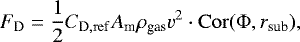
The general drag force FD is given by
 (4)
(4)
with drag coefficient CD and geometric cross section Am. The drag coefficient is dependent on the flow (i.e., Reynolds number and Knudsen number dependent, and can be separated in different regimes) (e.g., Whipple 1972), as shown in Fig. 5: the Stokes drag regime (III), a transition regime with an additional Reynolds number dependent correction term (Shiller & Naumann 1935) (I), and the Newton drag regime. For a sphere CD can be given as
 (5)
(5)
For a sphere in a flow regime with Re < 1 the drag force turns into the well-known Stokes law:
 (6)
(6)
For 0.01 < Kn < 10, the drag laws of the continuum regime do not hold anymore and the Cunningham slip correction factor Cun(Kn) has to be applied:
 (7)
(7)
The experimentally determined constants are α = 1.231 ± 0.0022, β = 0.470 ± 0.0037, and ω = 1.178 ± 0.0091 (Hutchins et al. 1995). The drag force in this regime is (Cunningham & Larmor 1910)
 (8)
(8)
For Re < 1 this drag regime is often referred to as the Knudsen regime (IV in Fig. 5). For 1 < Re < 103 and 0.01 < Kn < 10 both the Cunningham and Reynolds-dependent correction terms must be applied (II in Fig. 5).
In a flow with Kn > 10 the Epstein drag law applies (V in Fig. 5)
 (9)
(9)
with the mean thermal velocity of the gas molecules vth. The corresponding drag coefficient of the Epstein drag regime is
 (10)
(10)
In this work, we refer to the drag coefficient of a sphere in the respective drag regime as CD,ref, including Reynolds and Knudsen number corrections.
3 Porous bodies
The volume filling factor Φ of a porous particle is defined as the ratio of the volume occupied by the material Vm to the total volume Vt of the particle:
 (11)
(11)
Compact grains have Φ = 1. For very fluffy particles the volume filling factor approaches zero, Φ → 0. The porosity Po is defined as the ratio of the void volume to the total volume, or
 (12)
(12)
The definition of the total volume Vt requires the size of the particle. This definition is not unambiguous for porous particles with arbitrary shapes (Sorensen 2011). Therefore, different definitions of radii are used throughout literature and might be more or less suited to describe drag forces. In the context relevant here, these are the following.
Maximum radius rmax: if an aggregate has a well-defined outer boundary, the maximum radius rmax from the center of volume characterizes a boundary with a solid free gas flow.
Volume equivalent radius rve: the volume equivalent radius of a porous body corresponds to the radius of a sphere with homogeneous density and the same volume of the particle mass:
![Mathematical equation: \begin{equation*}r_{\textrm{ve}} = \sqrt[3]{\frac{3}{4 \pi} V_{\textrm{m}}}.\end{equation*}](/articles/aa/full_html/2021/11/aa41582-21/aa41582-21-eq13.png) (13)
(13)
Radius of gyration rg: for a particle with known volumetric mass density distribution ρm(r), the radius ofgyration rg is defined as
 (14)
(14)
with aggregate mass m and center of mass rS. For aggregates built up from N monomers, the radius of gyration can be given as the mean quadratic distance from all monomer coordinates ri to the center of mass of the aggregate rS:
 (15)
(15)
Characteristic radius rc: a homogeneous sphere with radius R has a radius of gyration of  , Following this, Mukai et al. (1992) defined a characteristic radius rc. It gives the radius of an equivalent sphere with the same radius of gyration as the aggregate:
 (16)
(16)
This size of aggregates is used in the models of Okuzumi et al. (2009) and in the following works: e.g., Zsom et al. (2011), Okuzumi et al. (2012), Krijt et al. (2015), and Matthews et al. (2011). We also use the characteristic radius to define the total volume of the particle as  in Eq. (11).
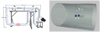 |
Fig. 1 Setup of the experiment. Left: schematics and dimensions of the wind tunnel. The part marked in red shows the location of the section for the drag measurements. Right: schematics of the measurement of the drag force: i refers to the initial state of the body; f refers to the state of the body when exposed to wind; αi,f is the angle between the two states. |
4 Experimental setup
4.1 Wind tunnel setup
A sketch of the wind tunnel setup is shown in Fig. 1. This wind tunnel has been used before by Küpper & Wurm (2015), among others, and in a smaller version by Paraskov et al. (2006). It consists of stainless steel tubes with an inner diameter of 320 mm. The total length of the wind tunnel is 18 m divided into several horizontal and vertical parts to achieve upward, downward, and horizontal winds. The wind tunnel can be evacuated and worked at a pressure between 0.01 mbar < p < 10 mbar.
4.2 Wind speed calibration
Gas flow is generated by a roots pump. At maximum power, the roots pump results in mean wind velocities of up to 100 m s−1 (Küpper & Wurm 2015). We limit the power and pressure to stay at a laminar wind profile with a Reynolds number of the experiment Re <2300, resulting in mean velocities  . The pump rate is pressure dependent. The wind speed was calibrated with a solid reference sphere with radius rmax = 1.5 cm. The drag acting on the sphere is within the range 1 < Re < 103 and 1 × 10⁻³ < Kn < 0.1. Therefore, the Cunningham correction factor was considered. The wind profile for a constant pump rotation frequency is shown in Fig. 2. The light red band shows the uncertainty, which mainly results from the 15% error of the used pressure sensor.
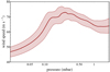 |
Fig. 2 Wind speed as a function of ambient pressure for the pump rotation frequency used. The thick red line indicates the speed calculated using a calibration sphere; the lighter red band shows the uncertainty. |
4.3 Force measurements
The porous bodies to be examined are placed at the bottom of the wind tunnel with a horizontal airflow. They are positioned in the center of the tube suspended by a thread which minimizes any unwanted gas interaction with a supporting structure. At the same time, the elongation of the particles can be observed through a side window and provides an easy measure of the drag force. When exposed to wind, the angle α between the initial relaxed position and the final equilibrium elongation is determined. With the gravitational acceleration g = 9.81 m s-2 the measured drag force Fm is
 (17)
(17)
The deflection angles are small but well measurable. The mean angle of all measurements is 4° with a standard deviation of 4°. Therefore, the deviation in the vertical direction is always <3 mm and the re-localization due to the aggregate’s deflection can be considered insignificant for the gas drag.
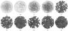 |
Fig. 3 Three-dimensional models of the porous bodies used in the experiments. |
4.4 Porous model aggregates
Three-dimensional models of the porous bodies used in the experiments are shown in Fig. 3. In light gray, an embedding sphere with radius rmax = 1.5 cm is shown. Figure 4 shows exemplary aggregates of the different wire and 3D printed models used in the experiment.
Models (a)–(d) are made of wire manually formed into a ball. The 3D models shown are examples displaying a random wire configuration with the same volumetric filling factor as the real bodies. Model (a) is made of tungsten wire with a diameter of 25 μm. Models (b), (c), and (d) are made of tungsten wire with a diameter of 100 μm.
Models (e)–(j) are made of 3D printed PETG cylinders that are randomly oriented and distributed, each connected to at least one other cylinder. The cylinders in models (e)–(f) each have a diameter of 1 mm, the cylinders in models (g)–(j) each have a diameter of 2 mm.
We define an area fraction of the aggregates Afrac as the covered area of the 2D projection of the aggregates Am (geometric cross section) compared to the cross section of a sphere of equivalent characteristic radius:
 (18)
(18)
Since the measured 2D projection depends on the orientation of the aggregates, we give the mean value and standard deviation of 70 projections of different rotation angles for models (e)–(j). For models (a)–(d), Af rac is estimated with the same method for 100 different simulated wire configurations with the same volumetric filling factors as the real porous bodies.
The volume filling factor is given by the mass of the aggregate mm divided by the mass of a sphere with radius rc (see Table 1) with equal volumetric mass density ρm:
 (19)
(19)
The projected area fraction, the volume filling factor, and the characteristic radius of each model are given in Table 1.
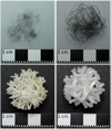 |
Fig. 4 Exemplary presentation of each type of aggregate used. Top left: rsub = 12.5 μm; top right: rsub = 50 μm; bottom left: rsub = 0.5 mm; bottom right: rsub = 1 mm. |
5 Results
The parameter space of our experiments is shown in Fig. 5. The red line shows the regime for the aggregates with L =rc = 1.3 cm. The other lines show the parameter range for the substructures of the porous bodies ranging from L =12.5μm to L = 1 mm (for those who would like to calculate the Reynolds and Knudsen numbers with the given sizes). The Re and Kn values for porous bodies are usually calculated with the characteristic radius as specific size, and we follow this definition throughout the paper. Figure 5 shows that the length scales of substructures and the overall size of the porous bodies are in different drag regimes. The pressure ranges from 5 × 10⁻² mbar ≤ p ≤ 1 mbar.
The measured forces for the different bodies can best be compared using the drag coefficients, which is defined by Eq. (4) or
 (20)
(20)
The drag coefficients CD are Reynolds number dependent. The data are shown in Fig. 6. As mentioned above, for porous bodies the specific length entering the Reynolds number is ill defined. We decided to use the characteristic radius rc for the determination of the Reynolds number.
Doing so, within the error bars, the functional behavior of the drag coefficients is similar for all aggregates. However, models (a)–(d) show significant deviations from the other models (i.e., they are strongly shifted). The drag coefficient for highly porous bodies is larger than expected.
In any case, the ratios of drag coefficients between porous bodies and reference sphere are essentially constant forall Reynolds numbers and are not pressure dependent (see Fig. 6). This allows one mean ratio to be given for the drag force between the porous body and reference sphere:  . The reference drag coefficient CD,ref is calculated according to Eq. (5) with L = rc. This ratio as a function of the filling factor is shown in Fig. 7.
The normalized drag coefficients show, that for low porosity aggregates and large substructures, the drag coefficient can be described by drag on a sphere with radius rc and a reduced cross section Afrac. However, the highly porous, low-substructure aggregates have much larger drag coefficients than one would expect from the reduced cross section. The coefficient is increased by a factor of up to 23 within the measured parameter space. More generally, an empirical description that fits the data is
 (21)
(21)
with
 (22)
(22)
The match of this expression to our experimental data as a function of the volumetric filling factor for each substructure in our experiment is shown in Fig. 7.
Equation (21) holds the condition, that CD,model is always at least the drag coefficient of a sphere with reduced cross section. It increases with decreasing volumetric filling factor Φ and decreases with the size of the substructure rsub.
Main properties of the model aggregates used.
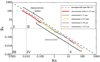 |
Fig. 5 Parameter space tested by the experiments. The roman numerals give the different drag regimes explained in Sect. 2. The red line shows the drag regime of the characteristic radius of the aggregates of ≈ 13 mm (see Table 1). The colored lines show the drag regime of the substructures used, as indicated in the figure legend. Here Kn and Re are calculated with different characteristic sizes L. The aggregates are associated with two different sizes and can therefore be affected by different flow regimes. |
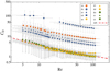 |
Fig. 6 Drag coefficient of the examined porous bodies as a function of the Reynolds number. We used L = rc to calculate Re. The red dashed line is the drag coefficient of a reference sphere. |
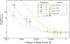 |
Fig. 7 Arithmetic mean of the drag coefficient normalized to the drag coefficient of the reference sphere as a function of the volume filling factors. The dashed lines show the model fits, as shown in Eq. (21). |
6 Discussion
The sub-structures for the highly porous aggregates in protoplanetary disks are in the Knudsen and Epstein regime. In a simple picture this should reduce the drag rather than increase it. It is unclear how far substructures are shielded from substructures ahead of them in wind direction which might have its share in an explanation.
We do not find any pressure dependency of the correction term, which would support the idea of just adding an additional Cunningham correction to the drag related to the substructures. Especially for the smallest substructures with Knudsen numbers of up to 100, this would lead to a dependence of CD (Re) not seen in Fig. 6. Therefore, currently, our model for the drag of porous bodies is merely empirical and is given as
 (23)
(23)
with the correction factor Cor as given in Eq. (22). Depending on the Reynolds and Knudsen number for the characteristic radius of the aggregate, the respective CD,ref has to be used. Following this and using  with Eqs. (9) and (10) for large and small Knudsen numbers and ignoring both the Re-transition regime and the Cunningham regime, we get the modified stopping times for aggregates:
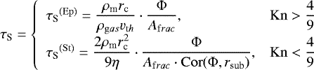 (24)
(24)
This is the stopping time often used multiplied by all the correction factors we identified that influence the drag of porous particles in Stokes drag regime: the volume filling factor Φ, the area fraction Af rac, and the substructure length scale rsub. In the Epstein regime we follow the estimation given by Okuzumi et al. (2012).
Although the aggregates used are not deformable or compactable, the increased gas drag in the Stokes regime may influence the evolution of porous particles (i.e., setting the collision velocity impacting the particle growth and collisional and static compaction). This may also apply to snowflakes in clouds on Earth and mineral aggregates in exoplanetary atmospheres (e.g., Ohno et al. 2020; Samra et al. 2020).
Understanding the drag of porous aggregates is of particular importance in planet formation. Highly porous aggregates have lower coupling times than their geometrical cross sections would suggest. This has implications for the collisional evolution and transport of grains in protoplanetary disks. The radial drift barrier, where grains are rapidly drifting inward has been recognized to be omnipresent since early work by Weidenschilling (1977). Porous growth has been one suggestion in recent years to overcome this barrier (Okuzumi et al. 2012; Laibe et al. 2012; Kataoka et al. 2013; Garcia & Gonzalez 2020).
It is probably one of the most extreme models of aggregate evolution that have been proposed in a series of papers by Okuzumi et al. (2009), Okuzumi et al. (2012), and Kataoka et al. (2013) where filling factors down to 10−5 are reached for centimeter-sized aggregates before they become slightly compressed. However, our results might amplify the underlying concepts. Gas grain coupling times are already small in their model. Considering our findings they might even be underestimated by large factors (up to tens), which would shift the onset of compaction to larger sizes. In addition, Garcia & Gonzalez (2020) followed the evolution of highly porous aggregates and the same consequences might apply here if modifications of the drag were considered.
Quite generally, there is little doubt that aggregation starts out fractal and highly porous (Blum & Wurm 2000; Wurm & Teiser 2021). As we find decreasing coupling times here, collision velocities are slower. This promotes longer phases of sticking and continuous porous growth, possibly on shorter timescales than the radial drift timescale (Okuzumi et al. 2012).
7 Conclusion
We studied the drag acting on porous aggregates composed of substructures of different sizes in a low-pressure wind tunnel. We find that porous bodies with micrometer-sized substructures are subject to drag forces that are larger by up to factors of tens compared to the usual values assumed. We give an empirical correction term depending on the sizes of the substructures rsub and the volume filling factor Φ to adjust the drag force laws of porous particles.
For highly porous bodies in planet formation, the coupling to the gas is faster than assumed. This slows down collision velocities and provides longer periods of porous growth before compaction occurs or particles are accreted by the star.
Acknowledgements
This project is funded by the Deutsche Forschungsgemeinschaft (DFG, German Research Foundation) - WU 321/16-1. We thank Satoshi Okuzumi for reviewing our work.
References
- Anderson, J. D. 2011, Fundamentals of Aerodynamics, 5th edn. (New York, NY: McGraw-Hill) [Google Scholar]
- Blum, J., & Wurm, G. 2000, Icarus, 143, 138 [NASA ADS] [CrossRef] [Google Scholar]
- Blum, J., & Wurm, G. 2008, ARA&A, 46, 21 [Google Scholar]
- Bogdan, T., Pillich, C., Landers, J., Wende, H., & Wurm, G. 2020, A&A, 638, A151 [EDP Sciences] [Google Scholar]
- Cunningham, E., & Larmor, J. 1910, Proc. R. Soc. London Ser. A, 83, 357 [NASA ADS] [CrossRef] [Google Scholar]
- Demirci, T., Kruss, M., Teiser, J., et al. 2019, MNRAS, 484, 2779 [NASA ADS] [CrossRef] [Google Scholar]
- Demirci, T., Schneider, N., Steinpilz, T., et al. 2020, MNRAS, 493, 5456 [NASA ADS] [CrossRef] [Google Scholar]
- Dullemond, C. P., & Dominik, C. 2004, A&A, 421, 1075 [NASA ADS] [CrossRef] [EDP Sciences] [Google Scholar]
- Garcia, A. J. L., & Gonzalez, J.-F. 2020, MNRAS, 493, 1788 [Google Scholar]
- Gonzalez, J.-F., Laibe, G., & Maddison, S. T. 2017, MNRAS, 467, 1984 [NASA ADS] [Google Scholar]
- Hutchins, D. K., Harper, M. H., & Felder, R. L. 1995, Aerosol Sci. Technol., 22, 202 [NASA ADS] [CrossRef] [Google Scholar]
- Jankowski, T., Wurm, G., Kelling, T., et al. 2012, A&A, 542, A80 [NASA ADS] [CrossRef] [EDP Sciences] [Google Scholar]
- Johansen, A., & Youdin, A. 2007, ApJ, 662, 627 [Google Scholar]
- Johansen, A., Blum, J., Tanaka, H., et al. 2014, in Protostars and Planets VI, eds. H. Beuther, R. S. Klessen, C. P. Dullemond, & T. Henning (Tucson: University of Arizona Press), 547 [Google Scholar]
- Kataoka, A., Tanaka, H., Okuzumi, S., & Wada, K. 2013, A&A, 557, L4 [NASA ADS] [CrossRef] [EDP Sciences] [Google Scholar]
- Kelling, T., Wurm, G., & Köster, M. 2014, ApJ, 783, 111 [Google Scholar]
- Krijt, S., Ormel, C. W., Dominik, C., & Tielens, A. G. G. M. 2015, A&A, 574, A83 [NASA ADS] [CrossRef] [EDP Sciences] [Google Scholar]
- Küpper, M., & Wurm, G. 2015, J. Geophys. Res. Planets, 120, 1346 [CrossRef] [Google Scholar]
- Laibe, G., Gonzalez, J.-F., & Maddison, S. T. 2012, A&A, 537, A61 [NASA ADS] [CrossRef] [EDP Sciences] [Google Scholar]
- Lyra, W., Youdin, A., & Johansen, A. 2021, Icarus, 356, 113831 [CrossRef] [Google Scholar]
- Matthews, L. S., Land, V., & Hyde, T. W. 2011, ApJ, 744, 8 [Google Scholar]
- Misener, W., Krijt, S., & Ciesla, F. J. 2019, ApJ, 885, 118 [NASA ADS] [CrossRef] [Google Scholar]
- Mukai, T., Ishimoto, H., Kozasa, T., Blum, J., & Greenberg, J. 1992, A&A, 262, 315 [Google Scholar]
- Ohno, K., Okuzumi, S., & Tazaki, R. 2020, ApJ, 891, 131 [Google Scholar]
- Okuzumi, S., Tanaka, H., & Sakagami, M.-a. 2009, ApJ, 707, 1247 [NASA ADS] [CrossRef] [Google Scholar]
- Okuzumi, S., Tanaka, H., Kobayashi, H., & Wada, K. 2012, ApJ, 752, 106 [NASA ADS] [CrossRef] [Google Scholar]
- Ormel, C. W., & Cuzzi, J. N. 2007, A&A, 466, 413 [NASA ADS] [CrossRef] [EDP Sciences] [Google Scholar]
- Paraskov, G. B., Wurm, G., & Krauss, O. 2006, ApJ, 648, 1219 [NASA ADS] [CrossRef] [Google Scholar]
- Perets, H. B., & Murray-Clay, R. A. 2011, ApJ, 733, 56 [Google Scholar]
- Pfeil, T., & Klahr, H. 2019, ApJ, 871, 150 [NASA ADS] [CrossRef] [Google Scholar]
- Riols, A., & Lesur, G. 2018, A&A, 617, A117 [NASA ADS] [CrossRef] [EDP Sciences] [Google Scholar]
- Ros, K., Johansen, A., Riipinen, I., & Schlesinger, D. 2019, A&A, 629, A65 [NASA ADS] [CrossRef] [EDP Sciences] [Google Scholar]
- Samra, D., Helling, Ch., & Min, M. 2020, A&A, 639, A107 [NASA ADS] [CrossRef] [EDP Sciences] [Google Scholar]
- Schneider, N., & Wurm, G. 2019, ApJ, 886, L36 [NASA ADS] [CrossRef] [Google Scholar]
- Schneider,N., Wurm, G., Teiser, J., Klahr, H., & Carpenter, V. 2019, ApJ, 872, 3 [NASA ADS] [CrossRef] [Google Scholar]
- Schneider, N., Musiolik, G., Kollmer, J. E., et al. 2021, Icarus, 360, 114307 [CrossRef] [Google Scholar]
- Sekiya, M., & Takeda, H. 2003, Earth Planets Space, 55, 263 [NASA ADS] [Google Scholar]
- Shiller, L., & Naumann, A. 1935, Zeitschrift des Vereins Deutscher Ingenieure, 77, 318 [Google Scholar]
- Simon, J. B., Armitage, P. J., Li, R., & Youdin, A. N. 2016, ApJ, 822, 55 [Google Scholar]
- Sorensen, C. M. 2011, Aerosol Sci. Technol., 45, 765 [NASA ADS] [CrossRef] [Google Scholar]
- Squire, J., & Hopkins, P. F. 2018, MNRAS, 823 [Google Scholar]
- Teiser, J., Engelhardt, I., & Wurm, G. 2011, ApJ, 742, 5 [NASA ADS] [CrossRef] [Google Scholar]
- Wada, K., Tanaka, H., Okuzumi, S., et al. 2013, A&A, 559, A62 [NASA ADS] [CrossRef] [EDP Sciences] [Google Scholar]
- Weidenschilling, S. J. 1977, MNRAS, 180, 57 [Google Scholar]
- Weidenschilling, S. J., & Cuzzi, J. N. 1993, in Protostars and Planets III, ed. E. H. Levy, & J. I. Lunine (Tucson: University of Arizona Press), 1031 [Google Scholar]
- Weidling, R., Güttler, C., Blum, J., & Brauer, F. 2009, ApJ, 696, 2036 [NASA ADS] [CrossRef] [Google Scholar]
- Whipple, F. L. 1972, in From plasma to planet (New York: Wiley Interscience Division), 211 [Google Scholar]
- Wurm, G., & Teiser, J. 2021, Nat. Rev. Phys. [Google Scholar]
- Wurm, G., Blum, J., & Colwell, J. E. 2001a, Phys. Rev. E, 64, 046301 [NASA ADS] [CrossRef] [Google Scholar]
- Wurm, G., Blum, J., & Colwell, J. E. 2001b, Icarus, 151, 318 [NASA ADS] [CrossRef] [Google Scholar]
- Wurm, G., Paraskov, G., & Krauss, O. 2005, Icarus, 178, 253 [Google Scholar]
- Yang, C.-C., Mac Low, M.-M., & Johansen, A. 2018, ApJ, 868, 27 [NASA ADS] [CrossRef] [Google Scholar]
- Youdin, A. N., & Goodman, J. 2005, ApJ, 620, 459 [Google Scholar]
- Zsom, A., Ormel, C. W., Güttler, C., Blum, J., & Dullemond, C. P. 2010, A&A, 513, A57 [NASA ADS] [CrossRef] [EDP Sciences] [Google Scholar]
- Zsom, A., Ormel, C. W., Dullemond, C. P., & Henning, T. 2011, A&A, 534, A73 [NASA ADS] [CrossRef] [EDP Sciences] [Google Scholar]
All Tables
All Figures
|
Fig. 1 Setup of the experiment. Left: schematics and dimensions of the wind tunnel. The part marked in red shows the location of the section for the drag measurements. Right: schematics of the measurement of the drag force: i refers to the initial state of the body; f refers to the state of the body when exposed to wind; αi,f is the angle between the two states. |
| In the text | |
|
Fig. 2 Wind speed as a function of ambient pressure for the pump rotation frequency used. The thick red line indicates the speed calculated using a calibration sphere; the lighter red band shows the uncertainty. |
| In the text | |
|
Fig. 3 Three-dimensional models of the porous bodies used in the experiments. |
| In the text | |
|
Fig. 4 Exemplary presentation of each type of aggregate used. Top left: rsub = 12.5 μm; top right: rsub = 50 μm; bottom left: rsub = 0.5 mm; bottom right: rsub = 1 mm. |
| In the text | |
|
Fig. 5 Parameter space tested by the experiments. The roman numerals give the different drag regimes explained in Sect. 2. The red line shows the drag regime of the characteristic radius of the aggregates of ≈ 13 mm (see Table 1). The colored lines show the drag regime of the substructures used, as indicated in the figure legend. Here Kn and Re are calculated with different characteristic sizes L. The aggregates are associated with two different sizes and can therefore be affected by different flow regimes. |
| In the text | |
|
Fig. 6 Drag coefficient of the examined porous bodies as a function of the Reynolds number. We used L = rc to calculate Re. The red dashed line is the drag coefficient of a reference sphere. |
| In the text | |
|
Fig. 7 Arithmetic mean of the drag coefficient normalized to the drag coefficient of the reference sphere as a function of the volume filling factors. The dashed lines show the model fits, as shown in Eq. (21). |
| In the text | |
Current usage metrics show cumulative count of Article Views (full-text article views including HTML views, PDF and ePub downloads, according to the available data) and Abstracts Views on Vision4Press platform.
Data correspond to usage on the plateform after 2015. The current usage metrics is available 48-96 hours after online publication and is updated daily on week days.
Initial download of the metrics may take a while.