| Issue |
A&A
Volume 655, November 2021
|
|
|---|---|---|
| Article Number | A64 | |
| Number of page(s) | 14 | |
| Section | Interstellar and circumstellar matter | |
| DOI | https://doi.org/10.1051/0004-6361/202141000 | |
| Published online | 18 November 2021 | |
Bayesian inference of three-dimensional gas maps
I. Galactic CO★
Institute for Theoretical Physics and Cosmology (TTK), RWTH Aachen University, Sommerfeldstr. 16,
52074
Aachen,
Germany
e-mail: pmertsch@physik.rwth-aachen.de
Received:
6
April
2021
Accepted:
5
July
2021
Carbon monoxide (CO) is the best tracer of Galactic molecular hydrogen (H2). Its lowest rotational emission lines are in the radio regime, and thanks to Galactic rotation, emission at different distances is Doppler shifted. For a given gas flow model, the observed spectra can thus be deprojected along the line of sight to infer the gas distribution. We used the CO-line survey of Dame et al. (2001, ApJ, 547, 792) to reconstruct the three-dimensional density of H2. We considered the deprojection as a Bayesian variational inference problem. The posterior distribution of the gas densities allowed us to estimate the mean and uncertainty of the reconstructed density. Unlike most of the previous attempts, we took the correlations of gas on a variety of scales into account, which allowed us to correct for some of the well-known pathologies, such as finger-of-god effects. The two gas flow models that we adopted incorporate a Galactic bar that induces radial motions in the inner few kiloparsecs and thus offers spectral resolution towards the Galactic centre. We compared our gas maps with those of earlier studies and characterise their statistical properties, for instance the radial profile of the average surface mass density.
Key words: Galaxy: structure / ISM: kinematics and dynamics / ISM: molecules / methods: statistical
Three-dimensional gas maps and their uncertainties are available at the CDS via anonymous ftp to cdsarc.u-strasbg.fr (130.79.128.5) or via http://cdsarc.u-strasbg.fr/viz-bin/cat/J/A+A/655/A64 and at https://zenodo.org/record/5501196
© ESO 2021
1 Introduction
Line surveys of molecular gas are a treasure trove for the study of the properties and dynamics of the interstellar medium (ISM; Ferrière 2001). While the dominant fraction of molecular gas is molecular hydrogen (H2), its line emission is inefficient in the cold and dense phase because of the large spacing of its energy levels. The energy levels of carbon monoxide (CO), on the other hand, are much more closely spaced, rendering it radiatively more efficient in the same environments. To first approximation, the density of H2 and CO are linearly related, making CO the preferred proxy for H2. In particular the J = 1 → 0 emission of 12CO at 115 GHz has become the observable of choice in the study of the molecular ISM in the Galaxy. While 12CO is almost always in the optically thick regime, the emission from its isotopologue 13CO is in the optically thin regime, thus complementary (e.g. Szűcs et al. 2014), but still bright enough to allow mapping over large regions of the Galaxy (e.g. Schuller et al. 2021).
Ever since its observational discovery (Wilson et al. 1970), the coverage, sensitivity, and angular resolution of CO surveys have continuously improved. Such surveys have enabled the study of the molecular ISM on scales as small as individual star-forming clumps of a few solar masses up to the total Galactic H2 mass of about 109M⊙. The applications of CO surveys thus range widely. Studies of Galactic structure on the largest scales, in particular of features such as spiral arms or nuclear bars, are interesting in their own right (Hou & Han 2014), but also offer invaluable clues for the theory of galaxy evolution (Kewley et al. 2019). The processes at play in the formation and dissolution of molecular clouds can be investigated through the study of individual clouds, but also through the statistical analysis of cloud catalogues (e.g. Miville-Deschênes et al. 2017). As stellar nurseries, the regions of dense molecular gas are central in the study of star formation (Kennicutt & Evans 2012). Due to its superior angular resolution compared to broad-band emission in other wavelengths, the correlation between different emission processes relies on precise information on the molecular phases. One concrete example is diffuse emission produced by non-thermal cosmic rays (Ackermann et al. 2012). Here, the molecular gas (together with atomic gas) provides the target for high-energy cosmic rays, resulting in the production of non-thermal gamma-ray emission either through bremsstrahlung or through the production and subsequent decay of pions into high-energy gamma-rays and neutrinos. While the study of all such processes in the Galaxy is interesting in its own right, it is also important to study and calibrate the correlations with other processes in order to use the observations of CO lines for extragalactic astrophysics (e.g. Sun et al. 2018).
As a result of our vantage point in the Galaxy, the galactic distribution of CO and H2 is not readily available from the gas-line surveys. However, because of Galactic rotation, different emission points along a line of sight in general posses different relative velocities with respect to the observer. Thus, the emission along a line of sight consists of aspectrum that encodes the distribution of emission with distance. The data products of gas-line surveys thus consist of spectra for individual lines of sight, oftentimes provided on a three-dimensional grid in longitude ℓ, latitude b, and velocity with respect to the local standard of rest (LSR), vLSR. For a given Galactic rotation curve, or more generally, given a gas flow model, such spectra can be deprojected in principle to find the three-dimensional distribution of CO and H2.
Unfortunately, several complications hamper the deprojection of the ℓbv-cubes of gas-line surveys into a three-dimensional xyz-cube of gas densities. First, along a given line of sight and for a given velocity, most gas-flow models exhibit two distance solutions inside the solar circle. For the velocity range affected by this effect, it is a priori unclear what fractions of the emission reside at the near and far distances. This effect is commonly referred to as the kinematic distance ambiguity. Second, for circular rotation, sight lines close to the Galactic centre (longitude ℓ ≃ 0°) and anti-centre (longitude ℓ ≃±180°) directions exhibit little to no radial velocity, thus lacking kinematical resolution: All the emission piles up around vLSR = 0 km s−1 and cannot be deprojected along the line of sight. Finally, peculiar velocities, that is, smaller-scale motions of gas on top of the large-scale gas flow, for instance due to stellar winds, supernova explosions, or spiral structures, perturb the smooth mapping of distance to radial velocity. These perturbations become visible as artefacts in the deprojected gas maps. Oftentimes, the inferred distribution of gas becomes smeared out along the line of sight, leading to the famous finger-of-god effect.
We illustrate the first two of these issues for the simple (and unrealistic) example of purely circular rotation. In this case, the radial velocity vLSR along (ℓ, b) for emission from the galacto-centric radius R is given by
 (1)
(1)
Further assuming a flat rotation curve, V (R) = 220 km s−1, we show vLSR as a function of position in the Galactic plane (b = 0°) in Fig. 1. We have assumed the observer to be located at Cartesian coordinates (x, y) = (R⊙, 0) with R⊙ = 8.15 kpc, and the relation from longitude ℓ, latitude b, and distance along the line of sight s to the Cartesian coordinates x, y, and z is

The lack of kinematic resolution around the Galactic centre and anti-centre direction is readily visible: each point along ℓ ≃ 0, ±180° is observed without any Doppler shift because there is no velocity component along the line of sight. It is also evident that the near-far ambiguity only affects positions within the solar circle, the circle centred on the Galactic centre with radius R⊙. Here, a given velocity vLSR < 0 (vLSR > 0) corresponds to two solutions for − 90° < ℓ < 0° (0° < ℓ < 90°). The two solutions are equidistant from the intersection of the line of sight with the tangent point circle: a circle of radius R⊙ ∕2, centred at (x, y) = (R⊙∕2, 0), the locus of points that are tangent to lines of constant longitude. For a given line of sight, the tangent point is an extremum of vLSR.
Several previous attempts have been made to deproject the results of gas-line surveys into three-dimensional gas distributions, and each study had to adopt a way for solving the issues discussed above. As for the lack of kinematic resolution towards the Galactic centre and anti-centre, Nakanishi & Sofue (2006) adopted a circular gas-flow model, thus ruling out the possibility of directly reconstructing gas near ℓ = 0° and ℓ = 180°. Instead, they resorted to interpolations between sidelines with low but finite radial velocities, at least for this side of the Galactic centre. The regions beyond the Galactic centre with little to no kinematical resolution were excluded. Pohl et al. (2008) instead adopted the result of a numerical simulation (Bissantz et al. 2003) of the gas flow that includes non-circular motions. Towards theGalactic centre and anti-centre, this provides several finite kinematic solutions, which even aggravates the distanceambiguity, but also provides some kinematic resolution. Gas could thus also be constructed close to ℓ = 0° and ℓ = ± 180° without interpolation.
As for the near-far ambiguity, when we assume an exponential or Gaussian distribution of gas in the direction perpendicular to the plane of the disk, the emission at a fixed velocity in the inner Galaxy will have a latitude profile that is composed of two Gaussians. Performing fits to the latitude distribution in individual velocity bins thus allows us to determine the relative distribution of gas between the two distance solutions. This method is know as the double-Gaussian method, and a number of studies haveadopted this technique (e.g. Clemens et al. 1988). Both Nakanishi & Sofue (2006) and Pohl et al. (2008) have also used the double-Gaussian method to break the near-far degeneracy in their deprojection. Specifically, Pohl et al. (2008) iteratively deprojected limited velocity ranges, assuming a certain thermal width, until the residual velocity spectra agreed with observational noise. Some artefacts are clearly still present in their gas maps, however. Nakanishi & Sofue (2006), on the other hand, were able to suppress some potential artefacts, but at the cost of adopting a rather coarse resolution, given the level of detail and small-scale structure available in the CfA CO survey compilation.
An alternative to the deprojection that is able to evade the problems described above to a certain degree is forward-modelling. For this, a parametric model for the gas distribution needs to be produced. Recently, Jóhannesson et al. (2018) provided such models for atomic and molecular hydrogen and determined the free parameters by fits to existing survey data. The near-far ambiguity and the lack of kinematic resolution are both fixed in this case by assuming a coherent distribution of gas throughout the offending regions. The authors were able to constrain a large number of parameters by their fit, and the properties of the spiral arms bear some resemblance due to other complementary data sets. However, as the authors themselves admit, not all the gas implied from the survey data can be successfully deprojected, such that the gas maps are to be considered as a lower limit of the real gas maps.
An important additional physical constraint that the gas densities have to fulfil but which is not leveraged by any of the previous studies is the existence of correlations. These correlations must exist on a range of scales and are due to a variety of processes. On the largest scales, they are due to the large-scale structure of the disk and the spiral arms, thus they ultimately are consequences of the formation history and density waves (Shu 2016). On smaller scales, the correlations are determined by the turbulent nature of the interstellar medium (Kolmogorov 1941), affecting both the fluctuation of gas density and velocity, and also magnetic fields. When the three-dimensional gas density is modelled as a (Gaussian) random field, these correlation can be parametrised by the power spectrum of gas densities. There is some support for the hypothesis of a log-normal random field (Nordlund & Padoan 1999; Ostriker et al. 2001), thus we considered the log of gas densities to behave like a Gaussian random field. This reconstruction problem for the gas density under the priors of a given correlation structure is most conveniently formulated in a Bayesian framework. We note that with a general enough inference method, the parameters for the power spectrum do not need to be assumed, but can be determined by the inference method together with the gas density. In addition, the Bayesian inference method provides not only an estimate of the gas density, but also quantifies its uncertainty. To our knowledge, none of the previous studies provided such an uncertainty estimate.
When the existence of correlations is taken into account, it is hoped that gas densities for regions for which data are less constraining may be predicted, for example,along ℓ = 0° and ℓ = ±180°. The quality of the deprojected data for these regions is reflected in an increased uncertainty for these regions. Additionally, it can help break the near-far ambiguity: Because of the coherence on large scales, the two solutions with gas at different distances will not exhibit the same likelihood, and the inference algorithm will thus be able to distinguish between these solutions. Finally, taking the presence of observational noise into account in our inference method naturally allows denoising the observations.
The remainder of this paper is organised as follows: in Sect. 2 we briefly review the survey data, introduce the two gas-flowmodels we adopt, and present the Bayesian method adopted for the deprojection and our data model. Our results are shown in Sect. 3 in a variety of representations. We compare our gas maps and supplemental results with those of previous studies. We conclude in Sect. 4 and provide some thoughts about future directions of research. Details and supplemental information for one of the gas-flow models are provided in Appendix A.
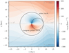 |
Fig. 1 Contour plot of the line-of-sight velocity vLSR for positions (x, y) in the Galactic plane, assuming purely circular motions with speed V (R) = 220 km s−1. We also indicate lines of fixed longitude (dotted) and the solar circle and the tangent point circle. |
2 Method
2.1 Survey data
We used the12CO (1 →0) line spectra as compiled by Dame et al. (2001). They comprise 37 individual surveys that were performed with two 1.2 meter millimeter-wave telescopes operated at Columbia University in New York City, NY, at the Centre for Astrophysics in Cambridge, MA, and at Cerro Tololo in Chile. Together, these surveys cover the entire Galactic plane in longitude, extending to ± 30° in latitude, thus covering virtually all areas for which significant emission has been reported. The velocity range is from − 319.8 to 319.8 km s−1 in velocity. Between individual surveys, the angular resolution varies from 1∕16 to 1∕2, as does the rms noise level, which we conservatively fixed to 0.3 K per channel. The survey data were downloaded from the SAO Radio Telescope Data Centre1.
Before publication, the raw survey data had been corrected for the motion of the Earth and the Sun with respect to the LSR. Since the time of publication of Dame et al. (2001), better estimates of these relative velocities have become available, however. Therefore we corrected the survey data by taking the updated parameter values into account as described in Sect. 4.2 of Wenger et al. (2018), adopting the parameter values of a recent parallax-based determination of the distances to ~ 200 masers (Reid et al. 2019). Specifically, we converted the standard Cartesian velocity component (U, V, W) = (10, 15, 7) km s−1 of the original surveys with the values (U′, V′, W′) = (10.6, 10.7, 7.6) km s−1 of model A5 of Reid et al. (2019). In Fig. 2 we show two projections of the corrected ℓbv-cube that is integrated over velocity, the so-called zero-moment map (top panel), and integrated over latitude, the ℓ − v diagram (bottom panel). In particular the ℓ-v diagram nicely illustrates the coherent structures that will help remedy some of the deficiencies of the usual deprojection techniques.
After the deprojection, we converted from the inferred CO emissivity into H2 gas density, adopting a linear relation between them. This relation is commonly assumed to exist between the H2 column density  and the velocity-integrated CO brightness temperature WCO ≡∫ dv Tb,
  , thus establishing the conversion factor XCO. While the relative abundances of H2 and CO depend on anumber of local factors (e.g. density, temperature, and metallicity), it is customary to adopt an average value of about
  . The value
  with an uncertainty of ±30% has been recommended (Bolatto et al. 2013). For a recent review of molecular gas surveys, see Heyer & Dame (2015).
2.2 Gas flow models
In addition to the three-dimensional gas density field that we wish to reconstruct, the distribution of CO brightness temperature in ℓ, b, and v depends on the three-dimensional velocity field, which is also unknown. While it might seem that the assumption of purely circular rotation is the most model-independent assumption possible, it is problematic in two ways: practically, as it does not provide any kinematic resolution towards the Galactic centre and anti-centre directions, and factually, as the gas flow is known not to be purely circular in the inner Galaxy because of the well-established presence of the Galactic bar (Blitz & Spergel 1991) that inducesradial motions in the inner few kiloparsec. While the existence of non-circular motions is qualitatively not challenged, the details are everything but certain.
In particular, we caution that the use of velocity fields based on simulations can be the source of significant artefacts if the modelled gas velocity differs from the true one. While this might seem an obvious point, it is easy to underestimate its importance because the effect of incorrect gas velocities on the reconstructed gas maps is aggravated by the particular form of the mapping between velocity vLSR and distance s: for regions with large gradients dvLSR∕ds, gas observed over velocityintervals ΔvLSR is reconstructed in relatively narrow intervals of the line-of-sight distance Δs, leading to regions of increased density. This can be considered the complement of an effect known as “velocity crowding2 ”. Simulated spiral arms typically exhibit these velocity gradients, and their positions will therefore be accentuated by increased gas densities. Even though the simulations that we adopted as a basis for our gas-flow models below were adjusted in order to reproduce the results from gas-line surveys to some extent, we currently cannot prevent these artefacts. In order to estimate the systematic uncertainty they cause, we therefore adopted two gas-flow models.
The first model is the result of a smoothed particle hydrodynamics simulation (Bissantz et al. 2003, hereafter BEG03). In addition to the gravitational potential of bulge and bar, some assumptions were made about the presence of spiral arms, in particular, a four-armed spiral structure was assumed. The Sun was assumed to be at a distance of 8 kpc from the Galactic centre, and an angle of 20° was adopted for the inclination of the major axis of the bar and the line Sun-Galactic centre. The resulting ℓ-v diagrams are similar to the CO data, but clearly miss some of the finer structure of the Dame et al. (2001) composite survey. We show their distribution of radial velocities in the top panel of Fig. 3. We extended the gas-flow model with a flat rotation curve beyond 8 kpc, in a similar fashion as Pohl et al. (2008). The assumed spiral arms are clearly visible in gradients in the velocity field. While newer simulations are available (e.g. Baba et al. 2010; Pettitt et al. 2014), we focussed here on BEG03 to allow a comparison of our results with those by Pohl et al. (2008), who used the same gas-flow model.
In addition, we constructed a gas-flow model based on a semi-analytical model for gas-carrying orbits in the potential dominated by the Galactic bar (Sormani et al. 2015, hereafter SBM15). We provide details of our model in Appendix A. The observer is assumed to be at a distance of 8.15 kpc from the Galactic centre (Reid et al. 2019), and the inclination of the major axis of the bar with respect to the line Sun-Galactic centre is again 20°. We show the resulting radial velocity map in the middle panel of Fig. 3 after rescaling the radial coordinate so as to bring the observer to the same galactocentric radius as in the BEG03 model in order to facilitate comparison. We also show the difference between the velocity fields of BEG03 and the SBM15 model in the bottom panel of Fig. 3. Three major differences are evident: First, while the overall agreement inside the solar circle is good, the agreement in the inner 2 kpc is less so. Second, the perturbations due to the spiral structure present in the model of BEG03 are clearly absent in our SBM15 model. The difference is mostly of about ±10 km s−1, but can be as large as ±30 km s−1 in limited regions. Finally, outside the solar circle, the difference in the adopted rotation curves is marked and can lead to differences as large as ±30 km s−1. We note, however, that there is little molecular gas at the relevant distances.
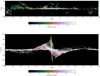 |
Fig. 2 Two-dimensional projections of the data from the Dame et al. (2001) compilation of surveys, after correcting for the updated local parameters. Top: velocity-integrated skymap of Galactic CO emission. Bottom: ℓ-v diagram of Galactic CO emission, integrated over latitudes from − 30° to 30°. |
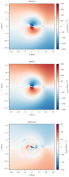 |
Fig. 3 Comparison of the two gas flow models that we adopted. Top: vLSR for the BEG03 model. Middle: vLSR for the SBM15 model. Bottom: difference between vLSR in the BEG03 and the SBM15 model. In all panels, the position of the Sun is marked with a cross. The color scale is different in the bottom panel. |
2.3 Bayesian inference
In deprojecting gas line surveys, we followed two connected goals: First, we wish to reconstruct the three-dimensional gas density under the constraint that the density possesses a certain spatial correlation structure. While we can be sure that these correlations exist, the details are poorly constrained, and ideally, we would hope for the data to constrain the correlation structure itself. Second, we would also like to obtain an estimate of the uncertainties. These two goals are most directly achieved by adopting a Bayesian framework.
We considered the deprojection of the three-dimensional gas density from line-survey data as a high-dimensional Bayesian inference problem, that is, we sought the posterior distribution of the gas density for the given the survey data. According to Bayes’ theorem (Bayes & Price 1763), the posterior is proportional to the likelihood, that is, the probability for the observed brightness temperature given the gas density, times the prior, that is, the probability of the gas density. We could constrain ourselves to finding the maximum of the posterior, but the maximum can be uninteresting if the posterior is multi-modal or has degenerate directions. In addition, we would need to estimate the uncertainty separately, for instance, by adopting the Laplace approximation (Laplace 1986), which equates the covariance at the maximum posterior position with the inverse Hessian. Instead, it is advantageous to keep track of the uncertainty while exploring the posterior.
Monte Carlo Markov chain (MCMC) methods (Hastings 1970) do exactly this, and they can approximate arbitrary posteriors given large enough sample sizes. However, with growing dimensionality, they become computationally expensive, and for the largedimensionality of the current problem, prohibitively so. Variational inference (Blei et al. 2017) instead approximates the posterior with a parametric distribution, for instance a multivariate Gaussian. The parameters of the parametric distribution can be determined if the “distance” between the approximate distribution and the true posterior can be estimated, for instance through the Kullback-Leibler divergence (Kullback 1968). For a multi-variate Gaussian, this would in principle involve the inversion of the large covariance matrix, which is again computationally prohibitive. Instead, it has been suggested (Knollmüller & Enßlin 2019) to approximate the covariance with the inverse Fisher information metric, a method known as metric Gaussian variational inference. This method has recently been applied to problems ranging from reconstruction of the three-dimensional dust density in the Galaxy from reddening data (Leike & Enßlin 2019) to radio interferometry (Arras et al. 2019).
In practice, this is implemented as an iterative scheme, alternating between estimating the covariance at the current mean and updating the mean for the current estimate of the covariance. Specifically, adopting standardisation of the parameters, the computation of the (inverse) Fisher information metric requires the Jacobian of the standardisation map. This can be obtained either analytically or numerically by automatic differentiation. The mean is estimated by minimising the Kullback-Leibler divergence with respect to the mean. This does not require explicitly computing the covariance matrix, which would entail the inversion of the Fisher information metric. Instead, the Kullback-Leibler divergence can be estimated stochastically, that is, by drawing samples from a Gaussian with the required covariance, which can be implemented with implicit operators. The application of the covariance in drawing the samples constitutes a linear system that can be solved by using a conjugate gradient algorithm.
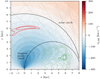 |
Fig. 4 Part of the galactic plane of Fig. 1. The radial velocity for circular rotation is shown by the shaded regions. Thecontour lines indicate the density of a simulated log-normal density field with a power-law power spectrum. The solar circle, the tangent point circle, and the lines of constant longitude are indicated. The dark green contours delineate a high-density feature at the near distance embedded in a large complex, shown by the light green contours. The red contours at the far distance mark a feature that would look similar in gas-line survey data, but would be penalised by the correlation structure assumed in the Bayesian inference approach. See text for a discussion of how the correlation structure of the density helps resolving the near-far ambiguity. |
2.3.1 Constraining power of correlations
A reconstruction of the molecular gas density that simultaneously considers all sight lines has the potential of leveraging the constrainingpower of the coherent nature of Galactic gas densities. This general idea has already been used in the denoising and deconvolution of other density fields from imperfect data. In our case, an additional benefit is that coherence can remedy the deficiencies of the kinematic reconstruction, that is, the lack of resolution towards the Galactic centre and anti-centre and the kinematic distance ambiguity. In order to gain some intuitive understanding for how exactly assuming coherence helps, we provide an illustration of how a specific simulated gas complex would be reconstructed.
In Fig. 4 we show a part of the Galactic plane of Fig. 1. As before, shaded areas indicate the radial velocity seen by an observer at (x, y) = (R⊙, 0) with R⊙ = 8.15 kpc, under the assumption of circular rotation. We overlaid a contour plot of a simulated gas density, with log-normal density and a power-law power spectrum. The solar circle and the tangent point circle are indicated in the same way as before, and in order to guide the eye, we also show lines of constant longitude for the observer at (x, y) = (R⊙, 0).
We now illustrate two ways of how the assumed correlation structure helps with reconstructing individual features in the gas density. Consider the dark green contours around (x, y) = (6, 1.8) kpc, which are the highest simulated density feature in this part of the plane. This structure is clearly located at the near distance. In a gas-line survey, this complex would be detected around longitude ℓ ≃ −40° and at velocities vLSR around − 50 and − 40 km s−1. Because of the kinematic distance ambiguity, however, emission around ℓ ≃−40° and vLSR = −50… −40 km s−1 could also be due to a structure at the far distance, in this case, roughly centred around (x, y) = (0, 6) kpc. We illustrate a structure that would contribute to line-survey data in a similar way by the red lines in Fig. 4. This structure is not part of the simulated density. It is very clear, however, that this structure is significantly distorted with respect to the original structure, in particular, it is much larger and very anisotropic. Such a large structure typically does not exist in the simulated density given the power spectrum that we adopted and will also not exist for the power spectrum that is inferred from the rest of the data in other parts of the plane. In the Bayesian inference scheme, the reconstruction of the structure at the far distance would therefore be penalised by the prior.
Second, the peak at the near distance, shown in dark green contours in Fig. 4, forms part of a larger extended structure, shown in light green contours. This is typical of the correlations at kiloparsec distances as parametrised by the power spectrum. Importantly, the kinematic distance of this extended structure is less uncertain because parts of this structure are close to the tangent point circle, where the kinematic distance is unambiguous. We note that the red contours, that is, the hypothetical reconstruction at the far distance, do not form part of this extended structure. (To see this, compare the red contours with the grey contours in its neighbourhood.) The prior therefore further penalises the reconstruction of this structure at the far distance.
The situation would be completely analogous for a structure that was truly at the far distance, in the sense that the typical size of the feature and its embedding in larger complexes would then lead to a preference of reconstruction at the far distance. If there is no clear preference of the near or far distance from the correlation structure, the inferred gas density maps will reflect this by an increased uncertainty at the respective near and far distance positions.
2.3.2 Data model
The relation between the CO emissivity ε(x, y, z) that we wish to reconstruct and the brightness temperature T(ℓ, b, v) from the Dame et al. (2001) survey is given by a linear map R from signal space (x, y, z) to data space (ℓ, b, v),
\,{=}\,\int_0^{\infty} \mathrm{d} s \, \varepsilon (\vec{r}) \, \delta(\varv - \varv_{\text{LSR}}(\vec{r})) \Big|_{\vec{r}\,{=}\,\vec{r}(\ell, b, s)} ,\end{equation*}](/articles/aa/full_html/2021/11/aa41000-21/aa41000-21-eq7.png) (5)
(5)
with r(ℓ, b, s) specified in Eqs. (2)–(4) above. Setting T = R[ε] would result in a deterministic likelihood p(T|ε),
![\begin{equation*} p(T_{\ell b \varv} | \varepsilon_{xyz})\,{=}\,\delta \left(T_{\ell b \varv} - R [ \varepsilon_{xyz} ] \right) , \end{equation*}](/articles/aa/full_html/2021/11/aa41000-21/aa41000-21-eq8.png) (6)
(6)
but we have to take additive noise n into account, which alters out data model to
![\begin{equation*} T_{\ell b \varv}\,{=}\,R [ \varepsilon_{xyz} ] + n_{\ell b \varv}.\end{equation*}](/articles/aa/full_html/2021/11/aa41000-21/aa41000-21-eq9.png) (7)
(7)
We assumed this noise to be Gaussian distributed, 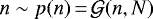 , with covariance N that is diagonal in harmonic space,
 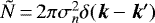 , that is, white noise. Given the properties of the individual surveys combined in Dame et al. (2001), we fixed σn = 0.3 K. We marginalised over the noise, thus obtaining a Gaussian likelihood,
![\begin{align*} \tilde{p}(T_{\ell b \varv} | \varepsilon_{xyz}) &\,{=}\, \int \mathrm{d}{n} \, p(T_{\ell b \varv} | \varepsilon_{xyz}, n_{\ell b \varv}) p(n_{\ell b \varv}) \\ &\,{=}\, \int \mathrm{d}{n} \, \delta \left(T_{\ell b \varv} - R [ \varepsilon_{xyz} ] - n_{\ell b \varv} \right) \mathcal{G}(n, N). \end{align*}](/articles/aa/full_html/2021/11/aa41000-21/aa41000-21-eq12.png)
Finally, we took into account that the measured v can differ from the actual radial velocity  of the emitting gas, for example due to thermal line width or turbulence. We took the difference
  to be normal distributed with variance
  and fixed σ = 5 km s−1. In principle,this requires another marginalisation, but we approximated this through a smearing of the linear map R instead,
![\begin{align*} & p(T_{\ell b \varv} | \varepsilon_{xyz}) \\ &\equiv \int \mathrm{d} \hat{\varv} \int \mathrm{d}{n} \, \delta \left(T_{\ell b \hat{\varv}} - R [ \varepsilon_{xyz} ] - n_{\ell b \varv} \right) \mathcal{G}(n, N) \mathcal{G}(\varv - \hat{\varv}, \sigma_{\varv}^2) \\ &\simeq \int \mathrm{d}{n} \, \delta \left(T_{\ell b \varv} - R\prime [ \varepsilon_{xyz} ] - n_{\ell b \varv} \right) \mathcal{G}(n, N) \\ &\,{=}\, \mathcal{G} \left(T_{\ell b \varv} - R\prime [ \varepsilon_{xyz} ], N \right) , \end{align*}](/articles/aa/full_html/2021/11/aa41000-21/aa41000-21-eq16.png)
![\begin{align*} R\prime [ \varepsilon_{xyz} ] &\equiv \int \mathrm{d} \hat{\varv} \, \mathcal{G}(\varv - \hat{\varv}, \sigma_{\varv}^2) R [ \varepsilon_{xyz} ] \\ &\,{=}\, \int_0^{\infty} \mathrm{d} s \, \varepsilon(\vec{r}) \, \mathcal{G}(\varv - \varv_{\text{LSR}}(\vec{r}), \sigma_{\varv}^2) \Big|_{\vec{r}\,{=}\,\vec{r}(\ell, b, s)}. \end{align*}](/articles/aa/full_html/2021/11/aa41000-21/aa41000-21-eq17.png)
To be able to define the posterior distribution, we still need to specify the signal prior. We modelled the CO emissivity ε(r) as a log-normal distributed random field, that is, s(r) ≡ ln(ε(r)∕ε0) is normal distributed. Under the assumption that s is statistically homogeneous, that is, the two-point correlation in configuration space, ⟨s(r)s(r′)⟩, is a function of the distance |r −r′| only, the two-point correlation in the harmonic domain becomes “diagonal”, that is,  where P(k) is the power spectrum. We further assumed that the power spectrum P(k) is isotropic, P(k) = P(k).
Instead of assuming a form for the power spectrum P(k), we would like to determine it during the reconstruction as well. Following Leike & Enßlin (2019), we therefore adopted a statistical model for the power spectrum, with a Gaussian-distributed normalisation y, a Gaussian distributed power-law index m, and add a Gaussian random field in log(k),
![\begin{align*} \sqrt{P(k)}\,{=}\,&\exp \left[ (\mu_y + \sigma_y \phi_y) + (\mu_m + \sigma_m \phi_m) \log(k) \right. \\ & \left. + \mathcal{F}^{-1} \!\! \left\{ \frac{a}{1 + t^2/t_0^2} \tau(t) \right\} \right]. \end{align*}](/articles/aa/full_html/2021/11/aa41000-21/aa41000-21-eq19.png)
Here, ϕy and ϕm are random variables and τ(t) a random field (in log(k)) that encode the power spectrum and are reconstructed at the same time as the signal itself.  represents the inverse Fourier transform from the variable t, that is, the conjugate of log(k). The parameters μy, σy, μm, σm, a, and t0 are meta-parameters, and we fixed them to the following values: μy = −13, σy = 0.1, μm = −4, σm = 0.1, a = 1, and t0 = 0.1. We stress that this representation of P(k) is flexible enough to closely approximate the true underlying power spectrum for k where the data are constraining enough; where they are not, the shape is interpolated or extrapolated.
Finally, assuming s to be a homogeneous random field must fail when the deviations from this assumption for the real gas density become too strong. This is certainly the case when considering the confinement of molecular gas to the Galacticplane. In order to not be biased in the reconstruction, we scaled the log-normal signal field εxyz with an exponential profile in z, exp [−|z|∕zh]. We adjusted zh to values such that the signal field εxyz averaged over different portions of the Galactic disk does not show strong gradients in the z direction and found zh = 40 pc to give satisfactory results. We also tested aGaussian profile ![$\exp[ - z^2/(2 \sigma_z^2) ]$](/articles/aa/full_html/2021/11/aa41000-21/aa41000-21-eq21.png) , but found the results to be virtually unchanged.
, but found the results to be virtually unchanged.
2.3.3 Details of the implementation
Because we performed our computations on a computer, the signal field is not a continuous field of gas densities, but rather a discretised version thereof. We adopted a Cartesian grid with the x, y, and z coordinates indexed with α, β, and γ, that is, εαβγ = ε(xα, yβ, zγ). Specifically, we considered a512 × 512 × 16 Cartesian grid stretching from − 16 kpc to 16 kpc in the x and y directions and from − 0.5 kpc to 0.5 kpc in the z direction, thus achieving a spatial resolution of 1∕16 kpc = 62.5 pc.
Beause the data are the spectra from a binned survey, they are already discretised, that is, Tijk = T(ℓi, bj, vk). We degraded the data from their native resolution on a 2880 × 481 × 493 grid to a 1440 × 241 × 247 grid. The discrete version of the linear map of Eq. (5) is
 (18)
(18)
Our data model, Eq. (7), can thus be represented by a multiplication with the sparse matrix  . For a specific implementation of the Gaussian variational inference, we made use of the nifty5 package3.
3 Results and discussion
The main result of our analysis are the three-dimensional gas maps obtained from the two gas-flow models and the corresponding uncertainties. Our gas maps provide the highest-resolution three-dimensional deprojections of CO gas-line surveys to date, with a number of robust and well-localised emission regions. They should prove useful in the study of Galactic structure and diffuse emission. We make our maps available to the community4.
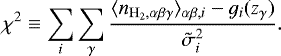
In Fig. 5 we show the projection of the H2 density onto the Galacticplane and its standard deviation for the BEG2003 gas-flow model (top panels) and the SBM15 gas-flow model (bottom panels). For each gas-flow model, the survey data were successfully deprojected into localised clusters of emission. The total reconstructed gas mass is 1.4 × 10⁹M⊙ for the BEG03 model and 1.3 × 10⁹M⊙ for the SBM15 model. This largely agrees with the value of (1 ± 0.3) × 109 M⊙ quoted by Heyer & Dame (2015).
Some elongated structures, spurs or spiral arm segments, are immediately visible. Some of the structures are more easily visible for the BEG03 model than for the SBM15 model. For instance, the two vertical spurs stretching from (x, y) = (4, −1) kpc to (x, y) = (4, 3) kpc and from (x, y) = (6, −1) kpc to (x, y) = (6, 3) kpc, respectively,are easily identified for the BEG03 model (top left panel of Fig. 5), but blend into a more extended emission for the SBM15 model. Revisiting Fig. 3 and in particular its bottom panel, it is clear that these structures are oftentimes linked to local extrema in the radial velocity field. For instance, the two spurs discussed above coincide with maxima of the velocity field of the BEG03 model, but are absent in the SBM15 model. They are due to the spiral arms, which have been put in by hand in the case of the BEG03 model, but not in the SBM15 model. We can also identify a spur that coincides with the tangent point circle, stretching from (x, y) = (2, −3) kpc to (x, y) = (6, −4) kpc. This is likely an artefact that indicates that the velocity range in the SBM15 model is too narrow.
Furthermore, a word of caution is in order concerning the interpretation of the extended density regions between (x, y) = (−3, 0) kpc and (x, y) = (3, 0) kpc in both maps as evidence for a Galactic bar. We note in passing that observations of external barred spirals oftentimes show evidence for an alignment of the molecular bar (if present) with a stellar bar. Examples are M 83 (Lundgren et al. 2004; Hirota et al. 2018), M 100 (Sempere & Garcia-Burillo 1997), NGC 4569 (Boone et al. 2007), and even doubled-barred spirals such as NGC 3504 (Kuno et al. 2000; Wu et al. 2021). For the Milky Way, determinations of the bar inclination angle indicate values between 20° (Queiroz et al. 2021) and 45° (Anders et al. 2019), but neither of these angles agrees with the vanishing inclination angle of the feature described above. We therefore hold our verdict as to the physicality of this feature. Some N-body simulations do not show the formation of a molecular bar associated with the stellar bar (e.g. Athanassoula et al. 2013).
We note that the reconstructed gas density comprises a rather wide dynamical range, as expected for a log-normal density. Some of the fainter features are therefore difficult to identify on a linear scale. In order to highlight them, we show the mean of the posterior, again projected onto the Galactic plane on a logarithmic colour scale in Fig. 6. We also overlaid a longitude grid and the contours of the respective radial velocities. This should facilitate an identification of certain features with the corresponding features in the ℓ − v-diagram of Fig. 2.
However, the mean of the posterior alone can be misleading because some of the localised features also have a rather large uncertainty. Unlike the previous deprojections, however, we now have a means of judging the validity of certain features by comparing the mean μ of the posterior with its uncertainty σ. To this end, we defined the signal-to-noise ratio (S/N) as μ∕σ. We show the S/N in Fig. 7, again for the BEG03 model in the top panel and in the bottom panel for the SBM15 model. Localised emission with an S/N of 3 or higher is clearly visible. In Fig. 7 we also overlaid the spiral arms, as determined from fits to a set of ~200 masers (Reid et al. 2019; see their Table 2 for the fitted spiral parameters.). Many of the local emission features obtained for either gas-flow model can be easily associated with a spiral arm: for the BEG03 model for all spiral arms, but most impressivelyfor the Norma, Sagittarius-Carina, Local, and Perseus arms. We comment on several noteworthy differences and similarities between the significant features obtained for the BEG03 and the SBM15 models below.
-
The gasdensity in the SBM15 model is generally more scattered and does not cluster in regions as large as the emissionin the BEG03 model. This is again due to the presence of local extrema in the radial velocity field in the BEG03 model, which boost the clustering. These local extrema are all but absent in the SBM15 model, and hence the gas density is less clustered.
-
Some of the spiral arms are obvious also for the SBM15 model, however, for instance, the segments along the Perseus and Sagittarius-Carina arms for galactocentric azimuths φ between ~200° and ~280°. Other examples are the segments along the Norma arm (90° ≲ φ ≲ 150°) and the local arm (330° ≲ φ ≲ 0°).
-
Some emission, in particular beyond the solar circle, is placed at different distances in the BEG03 and SBM15 models because of the different rotation curves adopted here. Given the rather small velocity gradient, this easily translates into differences of about a kiloparsec and thus affects the association with spiral arms. One example is emission around ℓ ~ 110° and withvLSR between − 60 and − 50 km s−1, see the bottom panel in Fig. 2. With the BEG03 model, this emission is located around (x, y) = (10, −6) kpc. With the SBM15 gas flow, this instead lies at (x, y) = (9.5, −5) kpc. In the former case, an association with the Norma arm suggests itself, in the latter case, the association with the Perseus arm is more likely.
In Fig. 8 we revisit the mass surface densities obtained with either gas-flow model (top panels) and compare them with the deprojections of Nakanishi & Sofue (2006) (bottom left) and Pohl et al. (2008) (bottom right). All gas densities are shown with the same dynamical range, but the mass surface density of Nakanishi & Sofue (2006) is significantly smoother. Some similarities are apparent between the map of Pohl et al. (2008) and our maps. This is even more so the case for our map that is based on the BEG03 model, the same gas-flow model asadopted by Pohl et al. (2008). However, there are also some differences:
-
The spiral arms are more homogeneous in Pohl et al. (2008). While in our reconstruction, the width is oftentimes varying along the segments, in the gas density of Pohl et al. (2008), some ring segments appear to have constant width. This might be an artefact of the particular algorithmic reconstruction chosen there.
-
An artefact that affects both the Pohl et al. (2008) map and our SBM15 map is the emission that is concentrated along an arc of the tangent point circle (see the discussion above).
-
The peak in the gas density reconstructed for both our gas-flow models near (x, y) = (−9, 2) kpc is absent in the Pohl et al. (2008) map, possibly because of the chosen suppression at large galactocentric radii and their enforcing of a vertical profile. We also note that our reconstruction places this feature at a rather large distance from the plane (~200 pc). Furthermore, an inspection of the v − ℓ-diagram shows that this feature has a very narrow line width, typical of local clouds with low masses. A similar conclusion might apply to the feature elongated between (x, y) = (−6, 2) kpc and (x, y) = (−6, 4) kpc in the BEG03 reconstruction.
-
Another class of artefacts that is apparent in the Pohl et al. (2008) maps is the features that are elongated along the lines of sight, the fingers-of-god, especially in regions of low gas densities. These are almost completely absent in our reconstructions.
-
Finally, Pohl et al. (2008) showed some gas density in regions where we found (almost) none, in particular beyond the solar circle. Unlike the structures that are solidly identified with spiral arms of the BEG03 model, some of these might be statistically not significant. This is to be compared with emission seen for our reconstruction in Fig. 6 near (x, y) = (−14, −1) kpc and (x, y) = (−14, −4) kpc, which is not statistically significant, see Fig. 7.
We conclude our discussion considering some properties of the derived distributions in galactocentric radius. In Fig. 9 we plot the surface mass density averaged in galactocentric rings Ri ≤ R < Ri+1, where Ri = iΔR with ΔR = 0.5 kpc. Close to the Galactic centre, the average gas density is a few tens of M⊙ pc−2 and it subsequently decreases towards r ≃ 3 kpc. Beyond, there is a local maximum at r ≃ 5 kpc, the well-established molecular ring (or possibly a convergence of spiral arms; Dobbs & Burkert 2012). Here, we find the average gas density to be ~1 M⊙ pc−2. Beyond, the gas density decreases further. While it appears to reach a plateau of 2 × 10⁻²M⊙ pc−2 around 12 kpc, we recall that we did not detect much significant emission beyond r ≃ 10 kpc.
We fitted Gaussian profiles ![$g_i(z) \propto \exp[-(z-z_{0,i})^2/2 \sigma_i^2]$](/articles/aa/full_html/2021/11/aa41000-21/aa41000-21-eq24.png) with means z0,i and standard deviations σi to the gas density distribution in the same galactocentric rings i as before by minimising the χ2 over all rings,
with means z0,i and standard deviations σi to the gas density distribution in the same galactocentric rings i as before by minimising the χ2 over all rings,
 (19)
(19)
Here,  denotes the averaging over all grid points αβ in the ith ring. We fixed the uncertainty
  to 0.15 of the maximum of
  for that particular ring i. For most rings, the Gaussian profile is a fair approximation, χ2 < 1. (Different z are correlated, hence χ2 is usually < 1.) For other rings, however, theaverage profile in z is only poorly described by a single Gaussian (see also Dame & Thaddeus 1985). We therefore removed these bins.
We show the full width at half maximum (FWHM), that is,  , a measure of the vertical extent of the gas distribution, as a function of galactocentric radius in the middle panel of Fig. 9 and compare it to a number of previous estimates. We note that our reconstructed gas densities appear to be more extended vertically, at least in the inner few kiloparsecs. Pohl et al. (2008) did not determine this parameter, but instead used it as an input for the analysis.
In the bottom panel of Fig. 9, we show the dependence of the midplane offset z0 on the galactocentric radius and again compare it to a number of previous estimates. While the general trend with galactocentric radius is thesame as seen in previous studies, our error bars are consistently smaller. We stress that the ensemble of samples from the posterior consists of full three-dimensional distributions, including uncertainties at individual positions and correlations between different positions. This enables statistical analysis beyond the axisymmetric quantities and simple error estimates.
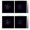 |
Fig. 5 Two-dimensional projection of reconstructed three-dimensional maps of molecular hydrogen. Top left: mean gas surface density Σ for the BEG03 gas-flow model. Top right: standard deviation of the gas surface density Σ for the BEG03 gas-flow model. Bottom left: mean gas surface density Σ for the SBM15 model. Bottom right: standard deviation of the gas surface density Σ for the SBM15 model. |
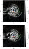 |
Fig. 6 Projected mean gas density Σ on a logarithmic colour scale, overlaying both contours in vLSR and a grid in longitude. Top: for the BEG03 gas flow model. Bottom: for the SBM15 model. |
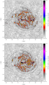 |
Fig. 7 Signal-to-noise ratio (S/N) of the mean gas density, with the spiral arms of Reid et al. (2019) overlaid. Top: For the BEG03 gas flow model. Bottom: For the SBM15 model. We also show a grid for the galactocentric azimuthal angle φ. |
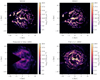 |
Fig. 8 Comparison of our two gas surface density reconstructions (top left and top right) with those of Nakanishi & Sofue (2006) (bottom left) and Pohl et al. (2008) (bottom right). |
4 Summary
We have presented a new deprojection of the CO line survey of Dame et al. (2001) with an unprecedented spatial resolution of 62.5 pc. This is based on a Gaussian variational Bayesian inference, which allows exploring the posterior distribution of this high-dimensional inference problem. While we assumed that correlations in configuration space exist, we did not assume any particular power spectrum, but determined the power spectrum during the reconstruction. We considered two gas-flow models that both take into account the presence of the Galactic bar, one based on a simulation of the gas flow in a predetermined potential (Bissantz et al. 2003, hereafter BEG03), the other based on a model for gas carrying orbits in the bar potential (Sormani et al. 2015, hereafter SBM15).
Our results are the three-dimensional distribution of molecular gas, assuming a fixed XCO factor of  . We have made our mean gas maps and their uncertainty available to the community4. We showed the mean and standard deviation of the gas density projected onto the Galactic plane and compared with previous studies. Unlike earlier studies, we have the capacity of distinguishing between statistically significant structures and noise artefacts. We found that some of the most prominent structures are affected by the assumed spiral structure in the BEG03 gas-flow model, but that significant coherent structures, some of which align with spiral arms (e.g. defined by parallax measurements of masers) are present in the SBM15 model as well. We projected some radial profiles out of the three-dimensional gas distribution and largely confirm the results of previous studies.
In the future, several extensions of the current analysis are noteworthy. After successfully applying our method to molecular line surveys to determine the H2 density, it would be interesting to apply it to surveys of atomic hydrogen, such as the recently completed HI4PI survey (HI4PI Collaboration 2016). While the HI distribution is known to show less clustering than molecular hydrogen, we are optimistic that the advantages of our approach will apply here as well. In addition, several shortcomings of the present study are due to our ignorance of the gas flow. If the velocity field could be determined at the same time as the gas density, these deficiencies could be remedied. We can envisage two ways to help regularise this underdetermined problem: Data from the parallax measurements (Reid et al. 2019) could be included, thus providing at least some loci to which the velocity field could be anchored. In addition, the physical correlation between gas densities and flow velocities could link the reconstruction of the two fields, which would require additional model inputs, however.
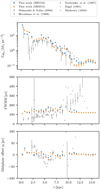 |
Fig. 9 Radial profiles of the surface mass density |

Acknowledgements
We thank the anonymous referee for her/his constructive comments that helped improve the quality of this paper.
Appendix A Semi-analytical gas-flow model
Short of running our own hydrodynamical simulations of gas flow in a barred potential, we employed a semi-analytical approximation to the gas flow. It has been hypothesised by Binney et al. (1991) that gas in the potential of a rotating bar slowly drifts towards thecentre, moving on orbits from two classes of closed orbits, so-called x1 and x2 orbits. The transition from the outer x1 orbits to theinner x2 orbits takes place through a shock structure that forms along a critical cusped orbit. Beyond this, the x1 orbits self-intersect, but the gas instead drifts on x2 orbits. This picture was observed in early simulations (Athanassoula 1992), but with limited resolution and a somewhat different potential than assumed by Binney et al. (1991), and more recently confirmed for the same potential and with a high-resolution simulation (SBM15). We adopted the potential of SBM15, but slightly adjusted their parameters.
Specifically, we adopted a combination of a triaxial potential for the bar,
 (A.1)
(A.1)
with  and a razor-thin disk potential generated by the surface mass density,
 (A.2)
(A.2)
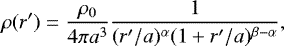
R denoting the cylindrical galactocentric radius. We adopted the following parameters: ρ0 = 0.69M⊙ pc−3, a = 1.8 kpc, α = 1.75, β = 3.5, Σ0 = 1.3 × 10³M⊙ pc−2, and R = 4.5 kpc (SBM15). We assumed a pattern speed of Ωp = 63 km s−1 kpc−1 for the rigidly rotating bar potential.
We solved the equations of motion for test particles in the combined potential using the galpy package5 (Bovy 2015). We find closed x1 and x2 orbits in the range of galactocentric radius ≤ 4 kpc. Some examples are shown in Fig. A.1.
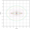 |
Fig. A.1 Some examples for x1 and x2 orbits found by solving for closed orbits in the rotating bar potential. The x1 orbits are marked by dashed and dot-dashed lines, and the x2 orbits are marked by solid and dotted lines. Gas is assumed to be moving on only a subset of these, i.e. on the orbits marked by a solid or dashed line. Orbits beyond the largest shown orbit are assumed to be circular. |
We interpolated the velocity field between the points on the x1 and x2 orbits for galactocentric radii R ≤ 4 kpc. While this works well for the regions inside the largest populated x2 orbit and outside the smallest populated x1 orbit, in between these orbits, the gas velocities are somewhat overestimated, see Fig. 5 of SBM15. We therefore added several nodes in the interpolation of the radial gas velocities to reach better agreement with Fig. 5 of SBM15.
Beyond 4 kpc, we assumed gas to move on circular orbits and the velocity to follow the “universal rotation curve” of Persic et al. (1996) with the updated parameters of Reid et al. (2019). A small suppression of 5 % was necessary to cause the rotation curve to connect smoothly with the interpolation at R = 4 kpc.
In the middle panel of Fig. 3 we show the radial velocity resulting from this semi-analytical gas-flow model. Even though we adopted slightly different parameters than SBM15, we refer to this model as the SBM15 model in the main text.
References
- Ackermann, M., Ajello, M., Atwood, W. B., et al. 2012, ApJ, 750, 3 [NASA ADS] [CrossRef] [Google Scholar]
- Anders, F., Khalatyan, A., Chiappini, C., et al. 2019, A&A, 628, A94 [NASA ADS] [CrossRef] [EDP Sciences] [Google Scholar]
- Arras, P., Frank, P., Leike, R., Westermann, R., & Enßlin, T. A. 2019, A&A, 627, A134 [NASA ADS] [CrossRef] [EDP Sciences] [Google Scholar]
- Athanassoula, E. 1992, MNRAS, 259, 345 [Google Scholar]
- Athanassoula, E., Machado, R. E. G., & Rodionov, S. A. 2013, MNRAS, 429, 1949 [Google Scholar]
- Baba, J., Saitoh, T. R., & Wada, K. 2010, PASJ, 62, 1413 [NASA ADS] [Google Scholar]
- Bayes, M., & Price, M. 1763, Philos. Trans. R. Soc. London Ser. I, 53, 370 [Google Scholar]
- Binney, J., Gerhard, O. E., Stark, A. A., Bally, J., & Uchida, K. I. 1991, MNRAS, 252, 210 [Google Scholar]
- Bissantz, N., Englmaier, P., & Gerhard, O. 2003, MNRAS, 340, 949 [NASA ADS] [CrossRef] [Google Scholar]
- Blei, D. M., Kucukelbir, A., & McAuliffe, J. D. 2017, J. Amer. Stat. Association, 112, 518 [Google Scholar]
- Blitz, L., & Spergel, D. N. 1991, ApJ, 379, 631 [Google Scholar]
- Bolatto, A. D., Wolfire, M., & Leroy, A. K. 2013, ARA&A, 51, 207 [CrossRef] [Google Scholar]
- Boone, F., Baker, A. J., Schinnerer, E., et al. 2007, A&A, 471, 113 [NASA ADS] [CrossRef] [EDP Sciences] [Google Scholar]
- Bovy, J. 2015, ApJS, 216, 29 [NASA ADS] [CrossRef] [Google Scholar]
- Bronfman, L., Cohen, R. S., Alvarez, H., May, J., & Thaddeus, P. 1988, ApJ, 324, 248 [NASA ADS] [CrossRef] [Google Scholar]
- Clemens, D. P., Sanders, D. B., & Scoville, N. Z. 1988, ApJ, 327, 139 [NASA ADS] [CrossRef] [Google Scholar]
- Dame, T. M., & Thaddeus, P. 1985, ApJ, 297, 751 [NASA ADS] [CrossRef] [Google Scholar]
- Dame, T. M., Hartmann, D., & Thaddeus, P. 2001, ApJ, 547, 792 [Google Scholar]
- Digel, S. 1991, Molecular clouds in the distant outer galaxy. PhD Thesis, Harvard Univ.: Cambridge, MA, USA [Google Scholar]
- Dobbs, C. L., & Burkert, A. 2012, MNRAS, 421, 2940 [NASA ADS] [CrossRef] [Google Scholar]
- Ferrière, K. M. 2001, Rev. Mod. Phys., 73, 1031 [NASA ADS] [CrossRef] [Google Scholar]
- Grabelsky, D. A., Cohen, R. S., Bronfman, L., Thaddeus, P., & May, J. 1987, ApJ, 315, 122 [CrossRef] [Google Scholar]
- Hastings, W. K. 1970, Biometrika, 57, 97 [Google Scholar]
- Heyer, M., & Dame, T. M. 2015, ARA&A, 53, 583 [Google Scholar]
- HI4PI Collaboration (Ben Bekhti, N., et al.) 2016, A&A, 594, A116 [NASA ADS] [CrossRef] [EDP Sciences] [Google Scholar]
- Hirota, A., Egusa, F., Baba, J., et al. 2018, PASJ, 70, 73 [CrossRef] [Google Scholar]
- Hou, L. G., & Han, J. L. 2014, A&A, 569, A125 [NASA ADS] [CrossRef] [EDP Sciences] [Google Scholar]
- Jóhannesson,G., Porter, T. A., & Moskalenko, I. V. 2018, ApJ, 856, 45 [CrossRef] [Google Scholar]
- Kennicutt, R. C., & Evans, N. J. 2012, ARA&A, 50, 531 [NASA ADS] [CrossRef] [Google Scholar]
- Kewley, L. J., Nicholls, D. C., & Sutherland, R. S. 2019, ARA&A, 57, 511 [Google Scholar]
- Knollmüller, J., & Enßlin, T. A. 2019, ArXiv e-prints [arXiv:1901.11033] [Google Scholar]
- Kolmogorov, A. 1941, Akademiia Nauk SSSR Doklady, 30, 301 [Google Scholar]
- Kullback, S. 1968, Information Theory and Statistics (New York: Dover Publication) [Google Scholar]
- Kuno, N., Nishiyama, K., Nakai, N., et al. 2000, PASJ, 52, 775 [NASA ADS] [CrossRef] [Google Scholar]
- Laplace, P. S. 1986, Stat. Sci., 1, 364 [NASA ADS] [CrossRef] [Google Scholar]
- Leike, R. H., & Enßlin, T. A. 2019, A&A, 631, A32 [NASA ADS] [CrossRef] [EDP Sciences] [Google Scholar]
- Lundgren, A. A., Wiklind, T., Olofsson, H., & Rydbeck, G. 2004, A&A, 413, 505 [NASA ADS] [CrossRef] [EDP Sciences] [Google Scholar]
- Malhotra, S. 1994, ApJ, 433, 687 [NASA ADS] [CrossRef] [Google Scholar]
- Miville-Deschênes, M.-A., Murray, N., & Lee, E. J. 2017, ApJ, 834, 57 [Google Scholar]
- Nakanishi, H., & Sofue, Y. 2006, PASJ, 58, 847 [NASA ADS] [Google Scholar]
- Nordlund, Å. K., & Padoan, P. 1999, in Interstellar Turbulence, eds. J. Franco, & A. Carraminana (Cambridge: Cambridge University Press), 218 [CrossRef] [Google Scholar]
- Ostriker, E. C., Stone, J. M., & Gammie, C. F. 2001, ApJ, 546, 980 [Google Scholar]
- Persic, M., Salucci, P., & Stel, F. 1996, MNRAS, 281, 27 [Google Scholar]
- Pettitt, A. R., Dobbs, C. L., Acreman, D. M., & Price, D. J. 2014, MNRAS, 444, 919 [NASA ADS] [CrossRef] [Google Scholar]
- Pohl, M., Englmaier, P., & Bissantz, N. 2008, ApJ, 677, 283 [NASA ADS] [CrossRef] [Google Scholar]
- Queiroz, A. B. A., Chiappini, C., Perez-Villegas, A., et al. 2021, A&A, in press, https://doi.org/10.1051/0004-6361/202039030 [Google Scholar]
- Reid, M. J., Menten, K. M., Brunthaler, A., et al. 2019, ApJ, 885, 131 [Google Scholar]
- Schuller, F., Urquhart, J. S., Csengeri, T., et al. 2021, MNRAS, 500, 3064 [Google Scholar]
- Sempere, M. J., & Garcia-Burillo, S. 1997, A&A, 325, 769 [Google Scholar]
- Shu, F. H. 2016, ARA&A, 54, 667 [NASA ADS] [CrossRef] [Google Scholar]
- Sormani, M. C., Binney, J., & Magorrian, J. 2015, MNRAS, 449, 2421 [NASA ADS] [CrossRef] [Google Scholar]
- Sun, J., Leroy, A. K., Schruba, A., et al. 2018, ApJ, 860, 172 [NASA ADS] [CrossRef] [Google Scholar]
- Szűcs, L., Glover, S. C. O., & Klessen, R. S. 2014, MNRAS, 445, 4055 [CrossRef] [Google Scholar]
- Wenger, T. V., Balser, D. S., Anderson, L. D., & Bania, T. M. 2018, ApJ, 856, 52 [Google Scholar]
- Wilson, R. W., Jefferts, K. B., & Penzias, A. A. 1970, ApJ, 161, L43 [NASA ADS] [CrossRef] [Google Scholar]
- Wu, Y.-T., Trejo, A., Espada, D., & Miyamoto, Y. 2021, MNRAS, 504, 3111 [NASA ADS] [CrossRef] [Google Scholar]
All Figures
|
Fig. 1 Contour plot of the line-of-sight velocity vLSR for positions (x, y) in the Galactic plane, assuming purely circular motions with speed V (R) = 220 km s−1. We also indicate lines of fixed longitude (dotted) and the solar circle and the tangent point circle. |
| In the text | |
|
Fig. 2 Two-dimensional projections of the data from the Dame et al. (2001) compilation of surveys, after correcting for the updated local parameters. Top: velocity-integrated skymap of Galactic CO emission. Bottom: ℓ-v diagram of Galactic CO emission, integrated over latitudes from − 30° to 30°. |
| In the text | |
|
Fig. 3 Comparison of the two gas flow models that we adopted. Top: vLSR for the BEG03 model. Middle: vLSR for the SBM15 model. Bottom: difference between vLSR in the BEG03 and the SBM15 model. In all panels, the position of the Sun is marked with a cross. The color scale is different in the bottom panel. |
| In the text | |
|
Fig. 4 Part of the galactic plane of Fig. 1. The radial velocity for circular rotation is shown by the shaded regions. Thecontour lines indicate the density of a simulated log-normal density field with a power-law power spectrum. The solar circle, the tangent point circle, and the lines of constant longitude are indicated. The dark green contours delineate a high-density feature at the near distance embedded in a large complex, shown by the light green contours. The red contours at the far distance mark a feature that would look similar in gas-line survey data, but would be penalised by the correlation structure assumed in the Bayesian inference approach. See text for a discussion of how the correlation structure of the density helps resolving the near-far ambiguity. |
| In the text | |
|
Fig. 5 Two-dimensional projection of reconstructed three-dimensional maps of molecular hydrogen. Top left: mean gas surface density Σ for the BEG03 gas-flow model. Top right: standard deviation of the gas surface density Σ for the BEG03 gas-flow model. Bottom left: mean gas surface density Σ for the SBM15 model. Bottom right: standard deviation of the gas surface density Σ for the SBM15 model. |
| In the text | |
|
Fig. 6 Projected mean gas density Σ on a logarithmic colour scale, overlaying both contours in vLSR and a grid in longitude. Top: for the BEG03 gas flow model. Bottom: for the SBM15 model. |
| In the text | |
|
Fig. 7 Signal-to-noise ratio (S/N) of the mean gas density, with the spiral arms of Reid et al. (2019) overlaid. Top: For the BEG03 gas flow model. Bottom: For the SBM15 model. We also show a grid for the galactocentric azimuthal angle φ. |
| In the text | |
|
Fig. 8 Comparison of our two gas surface density reconstructions (top left and top right) with those of Nakanishi & Sofue (2006) (bottom left) and Pohl et al. (2008) (bottom right). |
| In the text | |
|
Fig. 9 Radial profiles of the surface mass density |
| In the text | |
|
Fig. A.1 Some examples for x1 and x2 orbits found by solving for closed orbits in the rotating bar potential. The x1 orbits are marked by dashed and dot-dashed lines, and the x2 orbits are marked by solid and dotted lines. Gas is assumed to be moving on only a subset of these, i.e. on the orbits marked by a solid or dashed line. Orbits beyond the largest shown orbit are assumed to be circular. |
| In the text | |
Current usage metrics show cumulative count of Article Views (full-text article views including HTML views, PDF and ePub downloads, according to the available data) and Abstracts Views on Vision4Press platform.
Data correspond to usage on the plateform after 2015. The current usage metrics is available 48-96 hours after online publication and is updated daily on week days.
Initial download of the metrics may take a while.