| Issue |
A&A
Volume 653, September 2021
|
|
|---|---|---|
| Article Number | A105 | |
| Number of page(s) | 14 | |
| Section | Planets and planetary systems | |
| DOI | https://doi.org/10.1051/0004-6361/202040247 | |
| Published online | 15 September 2021 | |
TESS and HARPS reveal two sub-Neptunes around TOI 1062
1
Observatoire Astronomique de l’Université de Genève,
51 Ch. des Maillettes,
Sauverny,
1290
Versoix,
Switzerland
e-mail: This email address is being protected from spambots. You need JavaScript enabled to view it.
2
Institute for Computational Science, University of Zurich,
Winterthurerstr. 190,
8057
Zurich,
Switzerland
3
Center for Astrobiology (CAB, INTA-CSIC), Dept. de Astrofísica,
ESAC campus 28692 Villanueva de la Cañada
(Madrid),
Spain
4
Department of Physics and Kavli Institute for Astrophysics and Space Research, Massachusetts Institute of Technology,
Cambridge,
MA
02139,
USA
5
Department of Earth, Atmospheric and Planetary Sciences, Massachusetts Institute of Technology,
Cambridge,
MA
02139,
USA
6
Department of Aeronautics and Astronautics, MIT,
77 Massachusetts Avenue,
Cambridge,
MA
02139,
USA
7
Center for Astrophysics, Harvard & Smithsonian,
60 Garden Street,
Cambridge,
MA 02138,
USA
8
American Association of Variable Star Observers,
49 Bay State Road,
Cambridge,
MA 02138,
USA
9
Patashnick Voorheesville Observatory,
Voorheesville,
NY 12186,
USA
10
Tsinghua International School,
Beijing
100084,
PR China
11
Department of Astrophysical Sciences, Princeton University,
NJ
08544,
USA
12
NASA Ames Research Center,
Moffett Field,
CA 94035,
USA
13
Vanderbilt University, Department of Physics & Astronomy,
Nashville,
TN 37235,
USA
14
Astrophysics Science Division, NASA Goddard Space Flight Center,
Greenbelt,
MD 20771,
USA
15
Department of Astronomy, The University of Texas at Austin,
Austin,
TX 78712,
USA
16
Caltech/IPAC-NExScI,
M/S 100-22, 1200 E California Blvd,
Pasadena,
CA 91125,
USA
17
Instituto de Astrofísica e Ciências do Espaço, Universidade do Porto, CAUP, Rua das Estrelas,
4150-762
Porto,
Portugal
18
Departamento de Física e Astronomia, Faculdade de Ciências, Universidade do Porto,
Rua do Campo Alegre,
Porto,
Portugal
19
Department of Physics, University of Warwick,
Coventry
CV4 7AL,
UK
20
Centre for Exoplanets and Habitability, University of Warwick,
Gibbet Hill Road,
Coventry
CV4 7AL,
UK
21
SETI Institute,
Mountain View,
CA 94043,
USA
22
Space Telescope Science Institute,
3700 San Martin Drive,
Baltimore,
MD 21218,
USA
23
NCCR/PlanetS, Centre for Space & Habitability, University of Bern,
Bern, Switzerland
24
Department of Physics and Kavli Institute for Astrophysics and Space Research, Massachusetts Institute of Technology,
Cambridge,
MA
02139,
USA
25
Leiden Observatory, University of Leiden,
PO Box 9513,
2300 RA
Leiden,
The Netherlands
26
Department of Earth and Space Sciences, Chalmers University of Technology,
Onsala Space Observatory,
439 92,
Onsala,
Sweden
27
Aix Marseille Univ, CNRS, CNES, LAM,
Marseille,
France
28
European Southern Observatory,
Alonso de Córdova 3107,
Vitacura,
Santiago,
Chile
Received:
27
December
2020
Accepted:
5
May
2021
Abstract
The Transiting Exoplanet Survey Satellite (TESS) mission was designed to perform an all-sky search of planets around bright and nearby stars. Here we report the discovery of two sub-Neptunes orbiting around TOI 1062 (TIC 299799658), a V = 10.25 G9V star observed in the TESS Sectors 1, 13, 27, and 28. We use precise radial velocity observations from HARPS to confirm and characterize these two planets. TOI 1062b has a radius of 2.265−0.091+0.096 R⊕, a mass of 10.15 ± 0.8 M⊕, and an orbital period of 4.1130 ± 0.0015 days. The second planet is not transiting, has a minimum mass of 9.78−1.18+1.26 M⊕ and is near the 2:1 mean motion resonance with the innermost planet with an orbital period of 7.972−0.024+0.018 days. We performed a dynamical analysis to explore the proximity of the system to this resonance, and to attempt further constraining the orbital parameters. The transiting planet has a mean density of 4.85−0.74+0.84 g cm−3 and an analysis of its internal structure reveals that it is expected to have a small volatile envelope accounting for 0.35% of the mass at most. The star’s brightness and the proximity of the inner planet to what is know as the radius gap make it an interesting candidate for transmission spectroscopy, which could further constrain the composition and internal structure of TOI 1062b.
Key words: planets and satellites: general / planets and satellites: detection / planets and satellites: composition
© ESO 2021
1 Introduction
The Kepler mission was the first exoplanet mission to perform a large statistical survey of transiting exoplanets (Borucki et al. 2010; Howell et al. 2014); it impacted the field significantly with the detection of over 2300 exoplanets (see NASA Exoplanet Archive Akeson et al. 2013). Nevertheless, due to the faintness of the stars targeted by Kepler, only a small fraction are suitable for radial velocity (RV) follow-up. The Transiting Exoplanet Survey Satellite (TESS) has been designed to survey 85% of the sky for transiting exoplanets around bright, nearby stars (Ricker et al. 2015). It spent the first year of its mission searching for planets in the Ecliptic Southern Hemisphere. More than 2000 candidates have been detected and over 80 have been confirmed, expanding the number of small planets around cool stars (Guerrero 2020). RV follow-up programs have allowed us to quickly validate transiting planet candidates and to constrain their masses. Accurate measurements of the planetary mass and radius provide information on the planet’s bulk density. However, a full characterization on the planetary composition and internal structure is extremely challenging due to the degenerate nature of this problem, where various compositions and interiors can lead to the same average density. Nevertheless, by studying the population of planets in this mass and size range, it is possible to better understand the dominating processes of planet formation and evolution in a statistical manner (Alibert et al. 2010, 2015).
A key signature in the planet population is the hot Neptune desert, which corresponds to a lack of Neptune-mass planets close to their host stars (Szabó & Kiss 2011). The desert is likely to arise from a combination of photoevaporation and tidal disruption (Beaugé & Nesvorný 2013; Mazeh et al. 2016). At small orbital distances planets are subject to intense radiation from the host stars, and Neptune-like planets are probably not massive enough to retain their gaseous envelopes. An important advantage of the all-sky nature of TESS resides in its ability to find the brightest examples of stars hosting rare sub-populations of planets, such as the exoplanets lying inside the desert. TESS has been able to find the first planets deep inside the desert, for example TOI-849b (Armstrong et al. 2020), a recently discovered remnant core of a giant planet, and LTT9779b (Jenkins et al. 2020), an ultra-hot Neptune. The NCORES HARPS large program is designed to further study planets that may have undergone substantial envelope loss. Some of the recently discovered planets under this program include the mentioned TOI-849b and three mini Neptunes TOI-125b, c, d (Nielsen et al. 2020).
Another relevant feature in the exoplanet population is a lack of planets with radii between 1.5 R⊕ and 2 R⊕ (Fulton et al. 2017) known as the radius valley. This suggests that there is a transition between the super-Earth and sub-Neptune populations (Owen & Jackson 2012). This gap could be a result of stellar irradiation (Lopez & Fortney 2013) or core-powered mass-loss (e.g., Ginzburg et al. 2018), which leads to atmospheric evaporation that strips the planet down to its core or, alternatively, the consequence of a gas-poor formation (e.g., Gupta & Schlichting 2019). The observed features of the exoplanet populations are not well understood, and more exoplanet discoveries are crucial to reveal the overall picture of planets in the super-Earth and Neptune size and mass regimes.
In this paper we present the discovery and confirmation of two highly irradiated sub-Neptunes hosted by the TESS object of interest (TOI) 1062, a nearby (d = 82 pc) and bright (Vmag =10.2) G9V star (see Table 1 for a full summary of the stellar properties). We also used intensive radial velocity follow-up observations with HARPS to confirm the planetary nature of the transit detected in the TESS data and precisely determine the properties of the planetary system. The paper is organized as follows: in Sect. 2 we present the data collected on the system to discover and validate the planets, in Sect. 3 we analyze the host star fundamental parameters, and in Sect. 4 we characterize and discuss the planets. Our conclusions are presented in Sect. 5.
Stellar parameters of TOI-1062.
2 Observations
2.1 TESS photometry
TESS observed TOI 1062 (TIC 299799658) in Sectors 1 and 13 during the first year, and during Sectors 27 and 28 of the extended mission, obtaining data from 25 July to 22 August 2018, from 19 June to 17 July 2018, and from 4 July to 26 August 2020. The two-minute cadence data were reduced with the Science Processing Operations Center (SPOC) pipeline (Jenkins et al. 2016) adapted from the pipeline for the Kepler mission at the NASA Ames Research Center in order to produce calibrated pixels and light curves. On 29 September 2018 a transit candidate was announced around TOI 1062. TOI 1062.01 is a planet candidate with a period of 4.11506 ± 0.00002 days, a transit depth of 487.90 ± 45 ppm, and an estimated planet radius of 2.32 ± 0.46 R⊕. The candidate passed all the tests from the Threshold Crossing Event (TCE) Data Validation Report (DVR; Twicken et al. 2018; Li et al. 2019).
We used the publicly available Presearch Data Conditioning (PDC-SAP) flux time series (e.g., Twicken et al. 2010; Smith et al. 2012)provided by SPOC for the transit modeling, which is corrected for common trends and artifacts, for crowding, and for the finiteflux fraction in the photometric aperture. Figure 1 shows the 2 min cadence TESS light curve, along with the phase-folded curve for TOI 1062b.
2.2 Ground-based photometry with LCOGT
We obtained ground-based time series follow-up photometry of full transits of TOI 1062.01 on 24 August 2019 in i′ band and on 22 September 2020 in Pan-STARSS z-shortband from the Las Cumbres Observatory Global Telescope (LCOGT; Brown et al. 2013) 1.0 m network node at the South Africa Astronomical Observatory. We used the TESS Transit Finder, which is a customized version of the Tapir software package (Jensen 2013), to schedule the observations. The 4096 × 4096 LCO SINISTRO cameras have an image scale of 0.389″ per pixel, providing a field of view of 26′ × 26′. The standard LCOGT BANZAI pipeline was used to calibrate the images, and the photometric data were extracted with the AstroImageJ (AIJ) software package (Collins et al. 2017).
The initial i′-band observation intentionally saturated the target star to check for a faint nearby eclipsing binary (NEB) that could be contaminating the TESS photometric aperture. To account for possible contamination from the wings of neighboring star PSFs, we searched for NEBs out to 2.5′ from the target star. If fully blended in the SPOC aperture, a neighboring star that is fainter than the target star by 8.8 magnitudes in TESS band could produce the SPOC-reported flux deficit at mid-transit (assuming a100% eclipse). To account for possible delta-magnitude differences between TESS band and i′ band, we included an extra 0.5 magnitudes fainter (down to TESS-band magnitude 18.3). Our search ruled out NEBs in all 24 neighboring stars that meet our search criteria. Thez-shortband observation was defocused and exposed appropriately to measure the TOI 1062.01 light curve at high precision. For the data reduction process we used a 10.5″ radius aperture and selected four comparison stars with brightness comparable to that of the target star. The inner and outer radii of the background annulus were then set to the corresponding AIJ calculated values of 18.7″ and 28″, respectively. This combination was chosen as it minimized the amount of noise in the light curve. A 0.5 ppt transit, with model residuals of 0.3 ppt in 10 min bins, was detected in the uncontaminated target aperture.
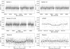 |
Fig. 1 TESS photometry from the of TOI 1062 from Sectors 1 (upper left), 13 (upper right), and Sectors 27 and 28 (middle left), and LCOGT photometry (middle right). The TESS light curves correspond to the PDC-SAP flux time series provided by SPOC. The TESS full light curve with the 2 min cadence data is shown in light gray, and the same data binnedto 10 min is in dark gray. The gaps in the data coverage are due to observation interruptions of the TESS spacecraft that occur after each TESS orbit of 13.7 days. The dots of the LCOGT are bigger for better visualization. The lower panels shows the phase-folded TESS light curves for TOI 1062b (left) and TOI 1062c (right) with the 2 min cadence data in light gray and binned to 10 min in black. We find that TOI 1062c does not transit. |
2.3 HARPS follow-up
We collected 90 high-resolution spectra of TOI 1062 using the High Accuracy Radial Velocity Searcher (HARPS) spectrograph mounted at the ESO 3.6 m telescope of La Silla Observatory, Chile (Mayor et al. 2003), with the goal of precisely determiningthe mass of the planet candidate and searching for additional planets in the system. The observations were carried out as part of the NCORES large program (ID 1102.C-0249, PI: Armstrong) between 31 August 2019 and 17 January 2020. HARPS is a stabilized high-resolution (R 115000) echelle spectrograph which can reach sub-m s−1 RV precision (Mayor et al. 2003). The instrument was used in high-accuracy mode (HAM), with a 1″ fiber on the star and another one to monitor the sky background. We used exposure times of 30 min.
The standard HARPS Data Reduction Software (DRS) was used to reduce the data, using a K0 mask for both the cross-correlation function (CCF; Pepe et al. 2002; Baranne et al. 1996) and the color correction, and reaching a typical signal-to-noise ratio per pixel of 60 and a photon-noise uncertainty of 1.4 m s−1. For each spectrum the usual activity indicators (S-index, Hα-index, Na-index, Ca-index,  ), the full width half maximum (FWHM), the line bisector, and the contrast of the CCF were measured.
2.4 High-resolution imaging
To check for the presence of contaminating stars in the TESS photometric aperture, TOI 1062 was observed on 14 January 2020 using the Zorro speckle imager (Scott 2019), mounted on the 8.1m Gemini South telescope in Cerro Pachon, Chile. Zorro uses high-speed electron-multiplying CCDs (EMCCDs) to simultaneously acquire data in two bands centered at 562 and 832 nm. Thedata is reduced following the procedures described in Howell et al. (2011), and provides output data including a reconstructed image and robust limits on companion detections. The contrast achieved in the resulting reconstructed image is shown in Fig. 2. We see that the Zorro speckle images reach a contrast of Δmag = 8.25 at a separation of 1.1″ in the 832 nm band, and cover a spatial range of 9.9–98.6 au around the star with contrasts between 5 and 8 mag in both bands, showing no close companions to TOI 1062b.
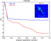 |
Fig. 2 Gemini/Zorro contrast curves and 1.2″ × 1.2″ reconstructed image of the 832 nm band. |
3 Host star fundamental parameters
3.1 Analysis of the spectrum
The stellar atmospheric parameters (Teff, log g, and [Fe/H]) and respective error bars were derived using the methodology described in Sousa (2014); Santos et al. (2013). Briefly, we make use of the equivalent widths (EWs) of iron lines, as measured in the combined HARPS spectrum of TOI 1062 using the ARES v2 code1 (Sousa et al. 2015), and we assume ionization and excitation equilibrium. This method makes use of a grid of Kurucz model atmospheres (Kurucz 1993) and the radiative transfer code MOOG (Sneden 1973). This approach leads to the following stellar parameters: Teff = 5328 ± 56K, [Fe/H] = 0.14 ± 0.04 dex, and logg = 4.55 ± 0.09. This is in agreement with the logg derived making use of the Gaia parallax and luminosity (Santos et al. 2004) which gives a value of 4.53. Using the Torres et al. (2010) calibration leads to a stellar mass of 0.94 ± 0.02 M⊙ and radius of 0.84 ± 0.09 R⊙. These values are used as priors in the global fit with juliet in Sect. 4.
3.2 Analysis of the spectral energy distribution
As an independent determination of the stellar parameters, we also performed an analysis of the broadband spectral energy distribution (SED) of the star together with the Gaia DR2 parallax (adjusted by + 0.08 mas to account for the systematic offset reported by Stassun & Torres 2018), in order to determine an empirical measurement of the stellar radius, following the procedures described in Stassun & Torres (2016), and Stassun et al. (2017, 2018). We pulled the BT VT magnitudes from Tycho-2; the BV i magnitudes from APASS; the JHKS magnitudes from 2MASS; the W1–W4 magnitudes from WISE; the G, GBP, GRP magnitudes from Gaia; and the near-ultraviolet (NUV) magnitude from GALEX. Together, the available photometry spans the full stellar SED over the wavelength range 0.2–22 μm (see Fig. 3).
We performed a fit using Kurucz stellar atmosphere models, using the effective temperature (Teff), metallicity ([Fe/H]), and surface gravity (logg) adopted from the spectroscopic analysis. The only additional free parameter is the extinction (AV), which we fixed to be zero due to the star’s proximity. The resulting fit is very good (Fig. 3) with a reduced χ2 of 1.8. The reduced χ2 is improved to 1.2 by excluding the GALEX NUV flux, which exhibits a modest excess; using the empirical relations of Findeisen et al. (2011), the GALEX NUV excess implies an activity level  , consistent with the spectroscopically determined value.
Integrating the (unreddened) model SED gives the bolometric flux at Earth, Fbol = 2.429 ± 0.057 × 10⁻⁹ erg s−1 cm−2. Taking the Fbol and Teff together with the Gaia DR2 parallax gives the stellar radius R⋆ = 0.838 ± 0.020 R⊙. In addition, we can use the R⋆ together with the spectroscopic logg to obtain an empirical mass estimate of M⋆ = 0.91 ± 0.19 M⊙, which is consistent with that obtained via empirical relations of Torres et al. (2010) and a 6% error from the empirical relation itself, M⋆ = 0.97 ± 0.06 M⊙. These values are in agreement with those derived from the spectral analysis in Sect. 3.1.
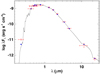 |
Fig. 3 Spectral energy distribution of TOI 1062. Red symbols represent the observed photometric measurements; the horizontal bars represent the effective width of the passband. Blue symbols are the model fluxes from the best-fit Kurucz atmosphere model (black). |
3.3 Rotational period and age
The stellar age can be derived from empirical rotation-age relations of Mamajek & Hillenbrand (2008). The HARPS calibration from the CCF-FWHM and the color index B-V gives v sin i = 2.13 ± 0.5 km s−1; then together with R⋆, we estimate the stellar rotation period Prot∕sini = 20.5 ± 2.9 d. In addition, Fig. 4 shows that the peak of the periodogram of the TESS light curves of Sectors 27 and 28 is at 21.82.4 days. The measured rotational modulation is nearly identical in the other TESS sectors. Another estimate of the expected rotation canbe inferred from the average value of the Ca II H & K chromospheric activity indicator for TOI 1062, which is  . Using the empirical relations in Mamajek & Hillenbrand (2008) we get a rotation period of 21.9
 days, in agreement with the result derived from the HARPS calibration and the modulation of the RAW light curves. Another way of constraining the rotational period of the star consists of fitting the RVs with time-dependent Gaussian processes (GPs). We use the celerite package (e.g., Foreman-Mackey et al. 2017) with a quasi-periodic kernel, and obtain a rotational period of
  days, which is in agreement with the previous estimations.
Using the rotational period obtained from the TESS data and the relations of Mamajek & Hillenbrand (2008), the age estimate is τ⋆ = 2.5 ± 0.3 Gyr. Because the vsini is a projected rotational velocity, we note that it is a lower limit on the true rotational velocity, so Prot∕sini is an upper limit on the true Prot, which implies that the age estimate above provides an upper limit to the stellar age.
We also attempted to derive the stellar age by making use of chemical clocks (e.g., Delgado Mena et al. 2019); however, weobtain a value much higher than with other methods described below. The reason is that the low Teff of TOI 1062 lies at the limit of applicability of such empirical relations, and thus we did not use the age provided by this method.
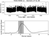 |
Fig. 4 TESS RAW photometric data of sectors 27 and 28 (top) and the corresponding periodogram. The peak of the periodogram shows a possible rotational modulation with a period of 21.8 days, which is in agreement with the rotational period obtained from HARPS calibration. |
3.4 Stellar abundances
Stellar abundances of refractory elements were derived using the classical curve-of-growth analysis method assuming local thermodynamic equilibrium (e.g., Adibekyan et al. 2012; Delgado Mena et al. 2017). Abundances of the volatile elements C and O were derived following the method of Delgado Mena et al. (2010); Bertran de Lis et al. (2015). Since the two spectral lines of oxygen are usually weak and the 6300.3Å line is blended with Ni and CN lines, the EWs of these lines were manually measured with the task splot in IRAF. All the [X/H] ratios are obtained by doing a differential analysis with respect to a high S/N solar (Vesta) spectrum from HARPS. The obtained values for this star are normal considering its metallicity except for the lower-than-expected value of oxygen. We find a high dispersion between both oxygen indicators that has to be taken with caution due to the difficulty of measuring reliable oxygen abundances for cool metal-rich stars. The stellar abundances of the elements are presented in Table 1.
3.5 Signal identification
In order to search for periodicities in the RV data we computed the l1 periodogram (e.g., Hara et al. 2017, 2020). This tool is designed to find periodicities in time series data corresponding to exoplanets detected using radial velocity data. It can be used similarly to a typical Lomb-Scargle periodogram or its variants (e.g., Baluev 2008), but it is based on a different principle. The l1 periodogram can analyze the radial velocity without the need to estimate the frequency iteratively, using the theory of compressed sensing adapted for handling correlated noise. Instead of fitting a sinusoidal function at each frequency as the Lomb–Scargle-type periodograms, the l1 periodogram searches directly for a representation of the input signal as a sum of sinusoids. As a result, all the frequencies of the signal are searched simultaneously. This relies on the so-called sparse recovery tools, which are designed to find a representation of an input signal as a linear combination of sine functions.
The l1 periodogram outputs a figure that has a similar aspect to that of a standard Lomb–Scargle-type periodogram, but with fewer peaks due to aliasing. We use the l1 periodogram of the HARPS data on a grid of frequencies between 0.01 and 0.3 cycles per day. In order to measure the significance of a possible signal the false alarm probability (FAP) is calculated, which encodes the probability of measuring a peak of a given height conditioned on the assumption that the data consists of Gaussian noise with no periodic component. Typically, a signal at the 1% FAP level is considered suggestive, and a 0.1% FAP level statistically significant. Figure 5 shows two l1 periodograms of the HARPS RVs. The top panel corresponds to the undetrended RVs. In this case we detect three significant signals at 4.11d (FAP 10−4%), 7.98 days (FAP 7.10−6%), and 26.6 days (FAP 3.10−5%). Although the coefficient amplitude of the second and third peaks are relatively close, their FAP values can differ significantly since it is estimated in a sequential manner: the highest peak is computed against zero, the second peak against the first, and the third peak against the second. Figure 6 clearly shows the effects of activity in the FWHM at the end of the time series. It suggests that the star was more active at that moment, probably due to one spot crossing event during one single rotational period, standing for only 20 days (from BJD 58 830–58 850). However, we find that the signal at 26.6 days disappears when we detrend the RVs using GP modeling with SPLEAF (e.g., Delisle et al. 2020) (see bottom panel of Fig. 5). The GP is trained on the  indicator, and then it is used to detrend the RVs using a linear fit. This method gives two significant peaks at 4.11d with FAP 6.10−5% and 8.00 days with FAP 4.10−4%.
Another way to detrend the stellar activity is to fit the correlations between activity indicators as the full width at half maximum (FWHM), the bisector or the S-index, and subtract them in order to correct for any long-term effects resulting from a magnetic cycle. We do so dividing the data into different time regimes selected in order to maximize the correlation of the RV data with the activity indicators in each bin. This approach also identifies two peaks at 4.11d with FAP 7.10−8% and 8.01 days with FAP 3.10−4%. Finally, we also find the same two significant signals when we do not use the data TBJD 58 730 –58 750, which corresponds to periods when the star was more active. The signal at 26.6 days only appears when using the full undetrended RV sample: it is clearly affected by stellar activity and it is within 1.6σ of the rotation period derived from the chromospheric activity indicator. We therefore conclude that only the peaks at ~4.11 days and ~8 days are caused by planets. In addition, even though the ~8-day signal is nearly double the ~4.11-day signal, in all the cases presented we find the 8-day signal after removing the ~4.11-day signal. We also evaluate the evidence of the second planet by comparing the difference in the Bayesian information criterion (ΔBIC) between the one-eccentric-planet and the two-eccentric-planets models. We obtain a value of ΔBIC = 11, which suggests strong evidence.
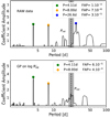 |
Fig. 5 Undetrended RVs (top) and detrended RVs (bottom) obtained via the
l1 periodogramusing Gaussian processes on the |

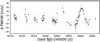 |
Fig. 6 Time series of the CCF-FWHM. |
3.6 Global fit with juliet
We determine the planetary parameters using the publicly available software juliet (e.g., Espinoza et al. 2019). juliet allows us to jointly fit the TESSand LCOGT photometry and the HARPS radial velocities with GP. The software is built on several publicly available tools used to model the photometric data (the batman package; Kreidberg 2015), the radial velocities (the radvel package; Fulton et al. 2018), and also to incorporate GP (the celerite package, Foreman-Mackey et al. 2017). The parameter space is explored using nested sampling, with the MultiNest algorithm (e.g., Feroz & Hobson 2008) in its Python implementation, PyMultiNest (e.g., Buchner et al. 2014). In addition, juliet computes the Bayesian evidence using dynesty (e.g., Speagle 2020), a Python package that estimates Bayesian posteriors and evidence using dynamic nested sampling. In short, nested sampling algorithms work as follows. The algorithm samples a number of live points randomly from the prior distribution, and the likelihood is evaluated at each of these points. At each iteration the point with the lowest likelihood is replaced by a new sampled point, keeping the number of live points constant. This process is continued until Bayesian evidence reaches a specified value. The number of live points used has to be large enough to adequately sample the parameter space.
The transit model fits the stellar density ρ⋆ together with the planetary and jitter parameters. For the stellar density we use the value obtained in Sect. 3, and the priors of the orbital parameters of the inner planet are taken from ExoFOP. We use the quadratic limb darkening coefficients (q1, q2) introduced by Kipping (2013) for the photometric data, since it was shown to be appropriate for space-based missions (Espinoza & Jordán 2015). In addition, instead of fitting the planet-to-star radius ratio and the impact parameter of the orbit, we use the parameterization introduced in Espinoza (2018) and fit the parameters r1 and r2 to make sure the full exploration of physically plausible values in the (p,b) space. We parameterize the eccentricity and the argument of periastron with  and
and  , always ensuring that e ≤ 1. We use the celerite aproximate Matern multiplied by exponential kernel to account for the stellar activity. The fit obtained with this kernel is nearly identical to the one obtained with other kernels as the quasi-periodic or the exp-sine-squared kernel.
We fit both planets with juliet and find no hint of transit for TOI 1062c, as shown in Fig. 1. The priors used are shown in Table 2, the final median planetary parameters determined by the juliet fit are listed in Table 3, and the RV fit is presented in Fig. 7. We find that TOI 1062b has an orbital period of 4.114 days, a radius of  R⊕, a mass of
  M⊕, and a density of
  g cm−3, slightly below the Earth’s mean density. Nevertheless, as discussed in detail in Sect. 5, its compositionand internal structure are unlikely to be similar to that of the Earth. We find an eccentricity of
  for TOI-1062b and 0.14 ± 0.07 for TOI-1062c. Figure 8 shows the eccentricity against the orbital period for the population of observed exoplanets from the NASA Exoplanet Archive, and we see that the TOI-1062b value is slightly higher than usual for itsorbital period. However, it may not be significant due to the bias towards higher eccentricities for nearly circular planets (Lucy & Sweeney 1971). TOI 1062 c instead is found to have an orbital period of 7.988 ± 0.04 days and a minimum mass of
  M⊕. TOI 1062 c is in nearly 2:1 motion resonance with its inner companion.
Prior parameter distribution of the global fit with juliet.
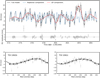 |
Fig. 7 HARPS RVs for TOI 1062 with a two planet model including eccentric orbits and Gaussian processes with Matern kernel. Top panel: RVs along with the residuals to the best fit right below the time series. Bottom panel: phase-folded data for each planet. The gray dots represent the observed RVs and the black dots the binned data. |
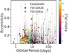 |
Fig. 8 Orbital eccentricity against orbital period for observed exoplanets from the NASA Exoplanet Archive. The color represents the planetary radius (see color scale at right). |
TOI-1062 parameters from juliet: median and 68% confidence interval.
4 Discussion
4.1 Internal structure
In order to characterize the internal structure of TOI 1062 b, we modeled its interior considering a pure-iron core, a silicate mantle, a pure-water layer, and a H-He atmosphere. The equations of state (EOSs) used for the iron core are from Hakim et al. (2018), the EOS of the silicate-mantle was calculated with PERPLE_X from Connolly (2009) using the thermodynamic data of Stixrude & Lithgow-Bertelloni (2011) and assuming Earth-like abundances, and the EOS for the H-He envelope are from Chabrier et al. (2019) assuming a proto-solar composition. For the pure-water layer we used the AQUA EOS from Haldemann et al. (2020). We assumed an envelope luminosity of L = 1022.52 erg s−1 (equal to Neptune’s luminosity). The thickness values of the planetary layers were set by defining their masses and solving the structure equations. To obtain the transit radius, we followed Guillot (2010) and evaluated the location where the chord optical depth τch is 2∕3. We did not use stellar abundances as an additional constraint since it is not clear whether they are a good proxy for the planetary bulk abundances (Wang et al. 2019; Plotnykov & Valencia 2020), and it has been shown that the stellar abundances are not always useful for constraining the internal composition (Otegi et al. 2020b).
Figure 9 shows M-R curves tracing the compositions of Earth-like planets (with a CMF = 0.33) and pure water subjected to a stellar radiation of F∕F⊕ = 230 (similar to that of TOI 1062 b). For reference, we also show exoplanets with accurate and reliable mass and radius determinations (Otegi et al. 2020a, accessible on the Data Analysis Center for Exoplanets, DACE2). TOI 1062 b sits above the Earth-like curve and below the pure-water curve, suggesting that it contains a small amount of volatile materials of less than 1% in mass. Figure 9 also displays the insolation flux relative to Earth against radii for the known exoplanets extracted from the NASA Exoplanet Archive, which shows the separate populations of super-Earths and mini-Neptunes. We see that TOI 1062 b sits in the mini-Neptune regime, close to the radius valley. In Otegi et al. (2020a) we identified two distinct populations, volatile-rich and “rocky” exoplanets (those expected to have small amounts of volatiles) separated by the water line. Using these results, we see that TOI 1062b lies in the rocky exoplanet regime defined in Otegi et al. (2020a), even if its radius is above the radius valley, suggesting that it is mostly composed of refractory materials by mass.
We used a generalized Bayesian inference analysis using a nested sampling scheme (Buchner et al. 2014) to quantify the degeneracy between various interior parameters and produce posterior probability distributions. Figure 10 shows ternary diagrams of the inferred composition of TOI 1062 b. The ternary diagram shows the degeneracy associated with the determination of the composition of exoplanets with measured mass and radius. We find a median H-He mass fraction of 0.1%, which corresponds to a lower bound since enriched H-He atmospheres are more compressed, and therefore increase the planetary H-He mass fraction. Formation models suggest that sub-Neptunes are likely formed by envelope enrichment (Venturini & Helled 2017). We also find that TOI 1062 b is expected to have a very significant iron core and silicate mantle, accounting for nearly 40% of the planetary mass and thicknesses of 1 R⊕ and 0.5 R⊕, respectively.The water layer has an estimated relative mass fraction of 15%. Nevertheless, the degeneracy between the core, silicate mantle, and water layer in this M-R regime is particularly high (Otegi et al. 2020b), and it does not allow accurate estimates of the masses of these constituents. Interior models cannot distinguish between water and H-He as the source of low-density material, so we also ran a three-layer model without the H2O envelope. Table 4 lists the inferred mass fractions of the core, mantle, water layer, and H-He envelope for the four-layer model and for the water-free model. In this case we find that the planet is 0.35% H-He, 26% iron, and 73% rock by mass, setting maximum limits for the atmospheric and rock mass since any water added would decrease these mass fractions.
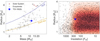 |
Fig. 9 Mass–radius and insolation–radius diagrams of observed exoplanets. Left: mass–radius diagram of exoplanets with accurate mass and radius determination from Otegi et al. (2020a). Also shown are the composition lines for Earth-like planets and pure water subjected to a stellar radiation of F∕F⊕ = 230 (similar to that of TOI 1062 b). Right: radius against insolation flux for known exoplanets from the NASA Exoplanet Archive. The colormap indicates the point density. TOI 1062 b is represented by a blue star. |
Inferred interior structure properties of TOI 1062b.
4.2 Dynamical analysis
As a general note for this section, the studies presented here were done under the hypothesis of a co-planar planetary system (i.e., the orbits ofplanets b and c evolve in the same plane). This is consistent with the observations, since TOI 1062c would not transit if it had the same orbital inclination as TOI 1062b.
4.2.1 Resonance
As can be seen from Table 3, the period ratio of the planets is Pc ∕Pb = 1.941. The planet pair thus lies close to the 2:1 mean-motion resonance (MMR). How close is the system to the MMR? We explore the structure of the parameter space of TOI-1062 near that resonance in order to investigate its dynamical state.
We therefore designed a two-dimensional section of the parameter space defined by the period ratio on one axis and the eccentricity of the outer planet ec on the other. Our section has a resolution of 101x101, meaning that we explore the dynamics of 10201 initial configurations defined by a unique set of (Pc ∕Pb,ec). All the other orbital parameters were initially fixed at the best values reported in Table 3. We numerically computed the future evolution of each configuration over 20 kyr. This was performed with the adaptive time-step high-order N-body integrator IAS15, which is available from the python package REBOUND (Rein & Liu 2012; Rein & Spiegel 2015). The perturbativeeffect of general relativity described in Anderson et al. (1975) was included via the library REBOUNDx (Tamayo et al. 2019). From these numerical simulations, the level of chaos of each configuration was evaluated with the Numerical Analysis of Fundamental Frequencies (NAFF) fast chaos indicator (Laskar et al. 1992; Laskar 1993). The result is presented in Fig. 11.
The NAFF computes precisely, for each planet, the average mean motion  over the two halves of the integration and compares these two estimations. Due to the secular constancy of the semi-major axis of regular orbits, this difference should be small in non-chaotic orbits. The higher the drift in the average mean-motion, the more chaotic the orbit. In this work we took as the NAFF of the system the maximum value of this drift over the planetary orbits in logarithmic scale,
 ![Mathematical equation: $\textrm{NAFF} ~ = ~ \max_i \left[\log_{10} \frac{\Delta n_i}{n_{0,i}}\right]$](/articles/aa/full_html/2021/09/aa40247-20/aa40247-20-eq19.png) , where the subscript i refers to the planet b or c, Δni is the drift of the average mean motion over the two halves of the integration, and n0,i is the initial mean motion of planet i. The color-coding in Fig. 11 depicts the NAFF defined above: the bluer colors indicate more regular systems. We also distinguish the strongly chaotic configurations from the ones that did not finish the integration because of either a close-encounter or an escape of a body (white boxes). We finally explain our choice of 20 kyr for the total integration time. Over this time span, the planetary orbits in the TOI-1062 system are expected to cover several secular cycles during which the semi-major axes oscillate. Covering several of these cycles allows to properly average the secular variations and isolate the chaotic diffusion. We verified numerically that several secular cycles are made up over an integration.
, where the subscript i refers to the planet b or c, Δni is the drift of the average mean motion over the two halves of the integration, and n0,i is the initial mean motion of planet i. The color-coding in Fig. 11 depicts the NAFF defined above: the bluer colors indicate more regular systems. We also distinguish the strongly chaotic configurations from the ones that did not finish the integration because of either a close-encounter or an escape of a body (white boxes). We finally explain our choice of 20 kyr for the total integration time. Over this time span, the planetary orbits in the TOI-1062 system are expected to cover several secular cycles during which the semi-major axes oscillate. Covering several of these cycles allows to properly average the secular variations and isolate the chaotic diffusion. We verified numerically that several secular cycles are made up over an integration.
In this map, the 2:1 mean motion resonance appears clearly as the orange band in the middle of the plot. For the current system’s parameters and the resolution of our chaoticity map, this resonance therefore seems chaotic. It is important to note that this picture is highly dependent on the system’s parameters. For instance, in this case the arguments of periastron ωb and ωc are close to the alignment. The opposite configuration where the orbits are anti-aligned would show a drastically different picture, with a different strength and apparent stability of the 2:1 MMR.
The two vertical lines depict the 1σ window of Pc. With the currently estimated orbital parameters and planet masses, the TOI 1062 system certainly lies outside of the 2:1 MMR. Despite the influence that a revision of the parameters may have on the resonance, it seems very unlikely that this conclusion will change.
Finally, we note that the uncertainty on the eccentricity of the inner planet eb is quite large. Modifying this parameter will directly impact the strength of the 2:1 MMR as the resonance width is expected to increase with the eccentricity. The same also applies for the planetary masses.
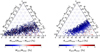 |
Fig. 10 Ternary diagram of the inferred internal composition of TOI 1062 b. We show the parameter space covered by the posterior distributions in the four-layer model in mass (left) and radius (right). |
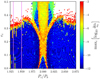 |
Fig. 11 Chaoticity map around the solution for the two-planet model (Table 3). The eccentricity of the outer planet ec and the period ratio Pc∕Pb are explored on a grid of 101 × 101 different configurations. A color is assigned to each box after a short numerical integration, according to its level of chaos using the NAFF indicator (see text). |
4.2.2 Stability constraints
While the chaoticity map presented above (Fig. 11) is informative about the maximum eccentricity of the outer planet allowed by orbital stability, this estimate should be considered with caution. This map explores the parameter space in two dimensions, without taking into account potential correlations with the other parameters. As already discussed, if the best-fit estimate of the other parameters changes, the entire map might change as well. In order to give proper stability constraints on the orbital parameters and masses of the planets, we also performed a global stability analysis from the posterior distribution of the joint photometry + RV analysis. The only fixed parameter is the inclination of the outer planet, taken equal to the inclination of the inner planet (i.e., we explored the co-planar case, which is compatible with the outer planet non transiting). We selected a sample of 10 000 solutions from that posterior. Each is numerically integrated over 20 kyr using the same integrator set-up described in the previous section. The level of chaos is again computed with the NAFF indicator. Over the 10 000 configurations, 8455 survived the entire 20 kyr simulation; the others were unstable (escape or close encounter of two bodies). Imposing a more strict stability threshold by further removing all solutions with NAFF > −5 leaves us with a stable posterior of 7224 configurations.
In any case, no stringent constraint can be added on the orbital parameters and masses of the planets. With the sorting in NAFF as defined above, only a slight cut in the eccentricities is observed. The new median estimates and 1σ confidence intervals are eb = 0.162 [0.098,0.228] and ec = 0.129 [0.065,0.205]. In particular, the global stability analysis does not allow us to further constrain the planetary masses (again assuming co-planar orbits).
4.3 Atmospheric characterization
TOI 1062b poses an interesting target for atmospheric characterization given its equilibrium temperature of ~1000 K. We expect a high-metallicity atmosphere for a planet with such a small radius and mass, as a result of the strong stellar irradiation received which would result in a significant loss of the H2 /He envelope. However, such a target is an excellent laboratory to study carbon chemistry at high temperature given its high expected metallicity. Beyond metallicities of ≳300× solar, the primary carbon bearing species in the atmosphere transitions from being CH4/CO to CO2 in thermochemical equilibrium (e.g., Moses et al. 2013). This planet is thus an ideal target to explore the CO, CH4, and CO2 chemical stability boundary which occurs at ~800 K in photospheric conditions at such high metallicities. The mean molecular weight for such an atmosphere at ~ 300× metallicity is expected to be ~4 g mol−1, and hence significant features are still present in transmission spectra compared to a solar metallicity atmosphere (at ~ 2.35 g mol−1). Using the transmission spectroscopy metric (TSM) defined in Kempton et al. (2018), we determine that TOI 1062b has a TSM value of 31.8 assuming a mean molecular mass of 2.3 g mol−1 and 18.3 assuming 4 g mol−1. The lower TSM value for the higher mean molecular weight is due to the reduced atmospheric scale height of a heavier atmosphere.This value is comparable to targets such as Trappist-1f and several simulated TESS targets from Sullivan et al. (2015).
On the other hand, TOI 1062b may have completely lost all of its H2 /He envelope which would result in an ultra-high-metallicity secondary atmosphere. At metallicities ≳ 3000× solar, the mean molecular weight of the heavier species such as CO2 and H2O now completely dominate due to the lack of significant H2 or He. Therefore, the mean molecular weight is likely to be >18 g/mol, and thus the scale height of spectral features in the transmission spectra are significantly reduced by a factor of ≳ 7× over a solar metallicity atmosphere. This reduces the TSM value for such an atmosphere to ≲5, making constraints on the abundances difficult. However, observations of the terminator may still be able to place a lower limit on the molecular weight, and thus the metallicity. They would also provide a direct contrast to planets such as 55 Cancri e which also indicate a high mean molecular weight atmosphere (Jindal et al. 2020). In addition, secondary eclipse spectroscopy for such a cool target is challenging, but has been achieved for GJ436b (Stevenson et al. 2010). However, for the case of TOI 1062b, the host star is a G-type and thus will result in a very weak planet–star flux contrast in emission spectroscopy.
5 Conclusions
We present the discovery of two new planets from the TESS mission in the TOI 1062 system. The analysis is based on 2 min cadence TESS observations from four sectors, ground-based follow-up from LCOGT, and RV data from the HARPS spectrograph. High-resolution imaging from Zorro speckle imager rules out the presence of nearby companions and potential nearby eclipsing binaries. We find that the host star is rotating with a period of 21.9 days, and also note the existence of a stellar spot whose lifetime is similar to the stellar rotational period.
TOI 1062b is expected to be a mini-Neptune with a period of 4.11 days, radius of 2.27 ± 0.1 R⊕, and mass of 10.2 ± 0.8 M⊕. Internal structure models indicate that TOI 1062b is expected to be composed of significant iron core and silicate mantle, accounting for nearly 40% of the planetary mass each, and that it is expected to have a small volatile envelope of 0.35% of the mass at most. TOI 1062c, which is not transiting, is found in the HARPS RV data. We find that its minimum mass is inferred to be 9.8 ± 1.2 M⊕, and that it is close to a 2:1 motion resonance with its inner companion, with a period of 7.97 days. The position of TOI 1062b with respect to the radius valley and its high equilibrium temperature of ~1000K make it an interesting candidate for atmospheric characterization. The strong stellar irradiation may result in a significant loss of the H-He envelope leaving a high-metallicity atmosphere that can be an excellent laboratory to study carbon chemistry at high temperature.
Acknowledgements
This work has been in particular carried out in the frame of the National Centre for Competence in Research ‘PlanetS’ supported by SNSF. D.J.A. acknowledges support from the STFC via an Ernest Rutherford Fellowship (ST/R00384X/1). This work was supported by FCT - Fundação para a Ciência e a Tecnologia through national funds and by FEDER through COMPETE2020 - Programa Operacional Competitividade e Internacionalização by these grants: UID/FIS/04434/2019; UIDB/04434/2020; UIDP/04434/2020; PTDC/FIS-AST/32113/2017 and POCI-01-0145-FEDER-032113; PTDC/FIS-AST/28953/2017 and POCI-01-0145-FEDER-028953. V.A. and E.D.M acknowledge the support from FCT through InvestigadorFCT contracts nr. IF/00650/2015/CP1273/CT0001, IF/00849/2015/CP1273/CT0003, respectively. C.D. acknowledges support from the Swiss National Science Foundation under grant PZ00P2_174028. Siddharth Gandhi acknowledges support from the UK Science and Technology Facilities Council (STFC) research grant ST/S000631/1. Resources supporting this work were provided by the NASA High-End Computing (HEC) Program through the NASA Advanced Supercomputing (NAS) Division at Ames Research Center for the production of the SPOC data products. We acknowledge the use of public TESS Alert data from pipelines at the TESS Science Office and at the TESS Science Processing Operations Center. This research has been partly funded by the Spanish State Research Agency (AEI) Projects No. ESP2017-87676-C5-1-R and No. MDM-2017-0737 Unidad de Excelencia “María de Maeztu”- Centro de Astrobiología (INTA-CSIC). S.G.S acknowledges the support from FCT through Investigador FCT contract nr. CEECIND/00826/2018 and POPH/FSE (EC). H.P.O. acknowledges that this work has been carried out within the framework of the NCCR PlanetS supported by the Swiss National Science Foundation. S.H. acknowledges support by the fellowships PD/BD/128119/2016 funded by FCT (Portugal). X.D is grateful to The Branco Weiss Fellowship–Society in Science for its financial support. This project has received funding from the European Research Council (ERC) under the European Union’s Horizon 2020 research and innovation programme (grant agreement No 851555/SCORE. A.O acknowledges support from an STFC studentship. S.H acknowledges CNES funding through the grant 837319.This work was supported by FCT through national funds (PTDC/FIS-AST/28953/2017) and by FEDER - Fundo Europeu de Desenvolvimento Regional through COMPETE2020 - Programa Operacional Competitividade e Internacionalização (POCI-01-0145-FEDER-028953) and through national funds (PIDDAC) by the grant UID/FIS/04434/2019. Funding for the TESS mission is provided by NASA’s Science Mission directorate. This work makes use of observations from the LCOGT network.
Appendix A HARPS spectroscopy
HARPS spectroscopy obtained between 31 August 2019 and 11 November 2019.
HARPS spectroscopy obtained between 20 November 2019 and 17 January 2020.
References
- Adibekyan, V. Z., Sousa, S. G., Santos, N. C., et al. 2012, A&A, 545, A32 [NASA ADS] [CrossRef] [EDP Sciences] [Google Scholar]
- Akeson, R. L., Chen, X., Ciardi, D., et al. 2013, PASP, 125, 989 [NASA ADS] [CrossRef] [Google Scholar]
- Alibert, Y., Mordasini, C., Benz, W., & Naef, D. 2010, EAS Pub. Ser., 42, 209 [NASA ADS] [CrossRef] [EDP Sciences] [Google Scholar]
- Alibert, Y., Thiabaud, A., Mzarboeuf, U., et al. 2015, AAS/Div. Extreme Sol. Syst. Abs., 47, 115.02 [NASA ADS] [Google Scholar]
- Anderson, J. D., Esposito, P. B., Martin, W., Thornton, C. L., & Muhleman, D. O. 1975, ApJ, 200, 221 [NASA ADS] [CrossRef] [Google Scholar]
- Armstrong, D. J., Lopez, T. A., Adibekyan, V., et al. 2020, Nature, 583, 39 [CrossRef] [Google Scholar]
- Baluev, R. V. 2008, MNRAS, 385, 1279 [NASA ADS] [CrossRef] [Google Scholar]
- Baranne, A., Queloz, D., Mayor, M., et al. 1996, A&AS, 119, 373 [NASA ADS] [CrossRef] [EDP Sciences] [Google Scholar]
- Beaugé, C., & Nesvorný, D. 2013, ApJ, 763, 12 [Google Scholar]
- Bertran de Lis, S., Delgado Mena, E., Adibekyan, V. Z., Santos, N. C., & Sousa, S. G. 2015, A&A, 576, A89 [NASA ADS] [CrossRef] [EDP Sciences] [Google Scholar]
- Borucki, W. J., Koch, D., & Kepler Science Team 2010, AAS/Div. Planet. Sci. Meeting Abs., 42, 47.03 [Google Scholar]
- Brown, T. M., Baliber, N., Bianco, F. B., et al. 2013, PASP, 125, 1031 [NASA ADS] [CrossRef] [Google Scholar]
- Buchner, J., Georgakakis, A., Nandra, K., et al. 2014, A&A, 564, A125 [NASA ADS] [CrossRef] [EDP Sciences] [Google Scholar]
- Chabrier, G., Mazevet, S., & Soubiran, F. 2019, ApJ, 872, 51 [NASA ADS] [CrossRef] [Google Scholar]
- Collins, K. A., Kielkopf, J. F., Stassun, K. G., & Hessman, F. V. 2017, AJ, 153, 77 [NASA ADS] [CrossRef] [Google Scholar]
- Connolly, J. A. D. 2009, Geochem. Geophys. Geosyst., 10, Q10014 [NASA ADS] [CrossRef] [Google Scholar]
- Delgado Mena, E., Israelian, G., González Hernández, J. I., et al. 2010, ApJ, 725, 2349 [NASA ADS] [CrossRef] [Google Scholar]
- Delgado Mena, E., Tsantaki, M., Adibekyan, V. Z., et al. 2017, A&A, 606, A94 [NASA ADS] [CrossRef] [EDP Sciences] [Google Scholar]
- Delgado Mena, E., Moya, A., Adibekyan, V., et al. 2019, A&A, 624, A78 [NASA ADS] [CrossRef] [EDP Sciences] [Google Scholar]
- Delisle, J. B., Hara, N., & Ségransan, D. 2020, A&A, 638, A95 [EDP Sciences] [Google Scholar]
- Espinoza, N. 2018, Res. Notes Am. Astron. Soc., 2, 209 [Google Scholar]
- Espinoza, N., & Jordán, A. 2015, MNRAS, 450, 1879 [Google Scholar]
- Espinoza, N., Kossakowski, D., & Brahm, R. 2019, MNRAS, 490, 2262 [NASA ADS] [CrossRef] [Google Scholar]
- Feroz, F., & Hobson, M. P. 2008, MNRAS, 384, 449 [NASA ADS] [CrossRef] [Google Scholar]
- Findeisen, K., Hillenbrand, L., & Soderblom, D. 2011, AJ, 142, 23 [Google Scholar]
- Foreman-Mackey, D., Agol, E., Ambikasaran, S., & Angus, R. 2017, AJ, 154, 220 [Google Scholar]
- Fulton, B. J., Petigura, E. A., Howard, A. W., et al. 2017, AJ, 154, 109 [Google Scholar]
- Fulton, B. J., Petigura, E. A., Blunt, S., & Sinukoff, E. 2018, PASP, 130, 044504 [NASA ADS] [CrossRef] [Google Scholar]
- Gaia Collaboration (Brown, A. G. A., et al.) 2018, A&A, 616, A1 [NASA ADS] [CrossRef] [EDP Sciences] [Google Scholar]
- Ginzburg, S., Schlichting, H. E., & Sari, R. 2018, MNRAS, 476, 759 [Google Scholar]
- Guerrero, N. 2020, Am. Astron. Soc. Meeting Abs., 235, 327.03 [NASA ADS] [Google Scholar]
- Guillot, T. 2010, A&A, 520, A27 [NASA ADS] [CrossRef] [EDP Sciences] [Google Scholar]
- Gupta, A., & Schlichting, H. E. 2019, MNRAS, 487, 24 [Google Scholar]
- Hakim, K., Rivoldini, A., Van Hoolst, T., et al. 2018, Icarus, 313, 61 [NASA ADS] [CrossRef] [Google Scholar]
- Haldemann, J., Alibert, Y., Mordasini, C., & Benz, W. 2020, A&A, 643, A105 [NASA ADS] [CrossRef] [EDP Sciences] [Google Scholar]
- Hara, N. C., Boué, G., Laskar, J., & Correia, A. C. M. 2017, MNRAS, 464, 1220 [NASA ADS] [CrossRef] [Google Scholar]
- Hara, N. C., Bouchy, F., Stalport, M., et al. 2020, A&A, 636, L6 [CrossRef] [EDP Sciences] [Google Scholar]
- Høg, E., Fabricius, C., Makarov, V. V., et al. 2000, A&A, 355, L27 [Google Scholar]
- Howell, S. B., Everett, M. E., Sherry, W., Horch, E., & Ciardi, D. R. 2011, AJ, 142, 19 [Google Scholar]
- Howell, S. B., Sobeck, C., Haas, M., et al. 2014, PASP, 126, 398 [NASA ADS] [CrossRef] [Google Scholar]
- Jenkins, J. M., Twicken, J. D., McCauliff, S., et al. 2016, Proc. SPIE, 9913, 99133E [Google Scholar]
- Jenkins, J. S., Díaz, M. R., Kurtovic, N. T., et al. 2020, Nat. Astron., 4, 1148 [Google Scholar]
- Jensen, E. 2013, Astrophysics Source Code Library [record ascl:1306.007] [Google Scholar]
- Jindal, A., de Mooij, E. J. W., Jayawardhana, R., et al. 2020, AJ, 160, 101 [Google Scholar]
- Kempton, E. M. R., Bean, J. L., Louie, D. R., et al. 2018, PASP, 130, 114401 [Google Scholar]
- Kipping, D. M. 2013, MNRAS, 435, 2152 [Google Scholar]
- Kreidberg, L. 2015, PASP, 127, 1161 [NASA ADS] [CrossRef] [Google Scholar]
- Kurucz, R. L. 1993, SYNTHE Spectrum Synthesis Programs and Line Data (Cambridge: Smithsonian Astrophysical Observatory) [Google Scholar]
- Laskar, J. 1993, Phys. D Nonlinear Phenom., 67, 257 [Google Scholar]
- Laskar, J., Froeschlé, C., & Celletti, A. 1992, Phys. D Nonlinear Phenom., 56, 253 [CrossRef] [Google Scholar]
- Li, J., Tenenbaum, P., Twicken, J. D., et al. 2019, PASP, 131, 024506 [NASA ADS] [CrossRef] [Google Scholar]
- Lopez, E., & Fortney, J. J. 2013, AAS/Div. Planet. Sci. Meeting Abs., 45, 200.08 [Google Scholar]
- Lucy, L. B., & Sweeney, M. A. 1971, AJ, 76, 544 [NASA ADS] [CrossRef] [Google Scholar]
- Mamajek, E. E., & Hillenbrand, L. A. 2008, ApJ, 687, 1264 [NASA ADS] [CrossRef] [Google Scholar]
- Mayor, M., Pepe, F., Queloz, D., et al. 2003, The Messenger, 114, 20 [NASA ADS] [Google Scholar]
- Mazeh, T., Holczer, T., & Faigler, S. 2016, A&A, 589, A75 [NASA ADS] [CrossRef] [EDP Sciences] [Google Scholar]
- Moses, J. I., Line, M. R., Visscher, C., et al. 2013, ApJ, 777, 34 [NASA ADS] [CrossRef] [Google Scholar]
- Nielsen, L. D., Gandolfi, D., Armstrong, D. J., et al. 2020, MNRAS, 492, 5399 [CrossRef] [Google Scholar]
- Otegi, J. F., Bouchy, F., & Helled, R. 2020a, A&A, 634, A43 [NASA ADS] [CrossRef] [EDP Sciences] [Google Scholar]
- Otegi, J. F., Dorn, C., Helled, R., et al. 2020b, A&A, 640, A135 [NASA ADS] [CrossRef] [EDP Sciences] [Google Scholar]
- Owen, J. E., & Jackson, A. P. 2012, MNRAS, 425, 2931 [Google Scholar]
- Pepe, F., Mayor, M., Rupprecht, G., et al. 2002, The Messenger, 110, 9 [NASA ADS] [Google Scholar]
- Plotnykov, M., & Valencia, D. 2020, MNRAS, 499, 932 [CrossRef] [Google Scholar]
- Rein, H., & Liu, S. F. 2012, A&A, 537, A128 [NASA ADS] [CrossRef] [EDP Sciences] [Google Scholar]
- Rein, H., & Spiegel, D. S. 2015, MNRAS, 446, 1424 [NASA ADS] [CrossRef] [Google Scholar]
- Ricker, G. R., Winn, J. N., Vanderspek, R., et al. 2015, J. Astron. Teles. Instrum. Syst., 1, 014003 [Google Scholar]
- Santos, N. C., Israelian, G., & Mayor, M. 2004, A&A, 415, 1153 [NASA ADS] [CrossRef] [EDP Sciences] [Google Scholar]
- Santos, N. C., Sousa, S. G., Mortier, A., et al. 2013, A&A, 556, A150 [NASA ADS] [CrossRef] [EDP Sciences] [Google Scholar]
- Scott, N. J. 2019, AAS/Div. Extreme Sol. Syst. Abs., 51, 330.15 [NASA ADS] [Google Scholar]
- Skrutskie, M. F., Cutri, R. M., Stiening, R., et al. 2006, AJ, 131, 1163 [NASA ADS] [CrossRef] [Google Scholar]
- Smith, J. C., Stumpe, M. C., Van Cleve, J. E., et al. 2012, PASP, 124, 1000 [Google Scholar]
- Sneden, C. A. 1973, PhD thesis, The University of Texas at Austin, USA [Google Scholar]
- Sousa, S. G. 2014, Determination of Atmospheric Parameters of B-, A-, F- and G-Type Stars, GeoPlanet: Earth and Planetary Sciences (Springer International Publishing (Cham)), eds. E. Niemczura, B. Smalley & W. Pych, 297 [Google Scholar]
- Sousa, S. G., Santos, N. C., Adibekyan, V., Delgado-Mena, E., & Israelian, G. 2015, A&A, 577, A67 [NASA ADS] [CrossRef] [EDP Sciences] [Google Scholar]
- Speagle, J. S. 2020, MNRAS, 493, 3132 [Google Scholar]
- Stassun, K. G., & Torres, G. 2016, AJ, 152, 180 [Google Scholar]
- Stassun, K. G., & Torres, G. 2018, ApJ, 862, 61 [Google Scholar]
- Stassun, K. G., Collins, K. A., & Gaudi, B. S. 2017, AJ, 153, 136 [Google Scholar]
- Stassun, K. G., Corsaro, E., Pepper, J. A., & Gaudi, B. S. 2018, AJ, 155, 22 [NASA ADS] [CrossRef] [Google Scholar]
- Stevenson, K. B., Harrington, J., Nymeyer, S., et al. 2010, Nature, 464, 1161 [NASA ADS] [CrossRef] [PubMed] [Google Scholar]
- Stixrude, L., & Lithgow-Bertelloni, C. 2011, Geophys. J. Int., 184, 1180 [NASA ADS] [CrossRef] [Google Scholar]
- Sullivan, P. W., Winn, J. N., Berta-Thompson, Z. K., et al. 2015, ApJ, 809, 77 [NASA ADS] [CrossRef] [Google Scholar]
- Szabó, G. M., & Kiss, L. L. 2011, ApJ, 727, L44 [NASA ADS] [CrossRef] [Google Scholar]
- Tamayo, D., Rein, H., Shi, P., & Hernandez, D. M. 2019, MNRAS, 491, 2885 [Google Scholar]
- Torres, G., Andersen, J., & Giménez, A. 2010, A&ARv, 18, 67 [Google Scholar]
- Twicken, J. D., Chandrasekaran, H., Jenkins, J. M., et al. 2010, Proc. SPIE, 7740, 77401U [NASA ADS] [CrossRef] [Google Scholar]
- Twicken, J. D., Catanzarite, J. H., Clarke, B. D., et al. 2018, PASP, 130, 064502 [Google Scholar]
- Venturini, J., & Helled, R. 2017, ApJ, 848, 95 [NASA ADS] [CrossRef] [Google Scholar]
- Wang, H. S., Liu, F., Ireland, T. R., et al. 2019, MNRAS, 482, 2222 [NASA ADS] [CrossRef] [Google Scholar]
- Wright, E. L., Eisenhardt, P. R. M., Mainzer, A. K. et al. 2010, AJ, 140, 1868 [Google Scholar]
The most recent version of the ARES code (ARES v2) can be downloaded at http://www.astro.up.pt/~sousasag/ares.
All Tables
All Figures
|
Fig. 1 TESS photometry from the of TOI 1062 from Sectors 1 (upper left), 13 (upper right), and Sectors 27 and 28 (middle left), and LCOGT photometry (middle right). The TESS light curves correspond to the PDC-SAP flux time series provided by SPOC. The TESS full light curve with the 2 min cadence data is shown in light gray, and the same data binnedto 10 min is in dark gray. The gaps in the data coverage are due to observation interruptions of the TESS spacecraft that occur after each TESS orbit of 13.7 days. The dots of the LCOGT are bigger for better visualization. The lower panels shows the phase-folded TESS light curves for TOI 1062b (left) and TOI 1062c (right) with the 2 min cadence data in light gray and binned to 10 min in black. We find that TOI 1062c does not transit. |
| In the text | |
|
Fig. 2 Gemini/Zorro contrast curves and 1.2″ × 1.2″ reconstructed image of the 832 nm band. |
| In the text | |
|
Fig. 3 Spectral energy distribution of TOI 1062. Red symbols represent the observed photometric measurements; the horizontal bars represent the effective width of the passband. Blue symbols are the model fluxes from the best-fit Kurucz atmosphere model (black). |
| In the text | |
|
Fig. 4 TESS RAW photometric data of sectors 27 and 28 (top) and the corresponding periodogram. The peak of the periodogram shows a possible rotational modulation with a period of 21.8 days, which is in agreement with the rotational period obtained from HARPS calibration. |
| In the text | |
|
Fig. 5 Undetrended RVs (top) and detrended RVs (bottom) obtained via the
l1 periodogramusing Gaussian processes on the |
| In the text | |
|
Fig. 6 Time series of the CCF-FWHM. |
| In the text | |
|
Fig. 7 HARPS RVs for TOI 1062 with a two planet model including eccentric orbits and Gaussian processes with Matern kernel. Top panel: RVs along with the residuals to the best fit right below the time series. Bottom panel: phase-folded data for each planet. The gray dots represent the observed RVs and the black dots the binned data. |
| In the text | |
|
Fig. 8 Orbital eccentricity against orbital period for observed exoplanets from the NASA Exoplanet Archive. The color represents the planetary radius (see color scale at right). |
| In the text | |
|
Fig. 9 Mass–radius and insolation–radius diagrams of observed exoplanets. Left: mass–radius diagram of exoplanets with accurate mass and radius determination from Otegi et al. (2020a). Also shown are the composition lines for Earth-like planets and pure water subjected to a stellar radiation of F∕F⊕ = 230 (similar to that of TOI 1062 b). Right: radius against insolation flux for known exoplanets from the NASA Exoplanet Archive. The colormap indicates the point density. TOI 1062 b is represented by a blue star. |
| In the text | |
|
Fig. 10 Ternary diagram of the inferred internal composition of TOI 1062 b. We show the parameter space covered by the posterior distributions in the four-layer model in mass (left) and radius (right). |
| In the text | |
|
Fig. 11 Chaoticity map around the solution for the two-planet model (Table 3). The eccentricity of the outer planet ec and the period ratio Pc∕Pb are explored on a grid of 101 × 101 different configurations. A color is assigned to each box after a short numerical integration, according to its level of chaos using the NAFF indicator (see text). |
| In the text | |
Current usage metrics show cumulative count of Article Views (full-text article views including HTML views, PDF and ePub downloads, according to the available data) and Abstracts Views on Vision4Press platform.
Data correspond to usage on the plateform after 2015. The current usage metrics is available 48-96 hours after online publication and is updated daily on week days.
Initial download of the metrics may take a while.