© ESO 2021

1. Introduction

Starting from the cosmological principle, assuming an isotropic and homogeneous Universe, a prominent observed dipole anisotropy in the cosmic microwave background (CMB) is assumed to be kinematic in nature. Other possible contributions from the integrated Sachs-Wolfe effect and primordial fluctuations are expected to be sub-dominant. As the assumption of an isotropic Universe should also hold true for its matter distribution, the observation of visible matter should show a similar effect of proper motion.

For radio galaxies, the proper motion of the Solar System affects the observed source counts, first predicted by Ellis & Baldwin (1984) and often described as the cosmic radio dipole. Several attempts have been made to measure the cosmic radio dipole in terms of radio continuum surveys, such as the NRAO VLA Sky Survey (NVSS; Condon et al. 1998) and Westerbork Northern Sky Survey (WENSS; de Bruyn et al. 2000). In order to measure the vector of cosmic radio dipole, a variety of estimators have been introduced, such as linear estimators that use only the position of the sources (Crawford 2009; Singal 2011; Gibelyou & Huterer 2012; Rubart & Schwarz 2013) or estimators that use source counts in spherical harmonics (Blake & Wall 2002; Tiwari & Nusser 2016). The results of these different estimators and surveys vary from consistent measurements based on the CMB to several times the amplitude. On the other hand, the measured dipole directions are consistent with the CMB dipole.

Contributions from local structure and Poisson noise are expected to change the measured cosmic radio dipole, whereas the structure-induced dipole is expected to be dominant for sources limited to a redshift of z ≪ 1. Nusser & Tiwari (2015) and Tiwari & Nusser (2016) presented a model of the dipole component of NVSS radio galaxies, for which about 70% of the observed dipole signal, after the solar motion is removed, is attributed to structures within z ≲ 0.1. However, apart from the contributions coming from cosmic structure and Poisson noise, the sdipole attributed to our proper motion should be dominant for a catalogue with a mean redshift of order unity and large sky coverage. The aim of this work is to revisit the properties of linear and quadratic dipole estimators and to present a unified analysis for four wide-area continuum radio surveys across a decade in frequency in order to reveal the nature of the cosmic radio dipole.

After introducing the kinematic dipole in Sect. 2, we discuss the possible biases of the estimated dipole direction and amplitude for a linear estimator in Sect. 3. In Sect. 4, we compare them to the properties of a quadratic estimator, introduced in Bengaly et al. (2019). The quadratic estimator is then applied to four different radio surveys, which are described and masked in Sect. 5. We show the results of our dipole estimates in Sect. 6. In Sect. 7, we test and discuss the frequency dependence of the dipole amplitude. We present our conclusions in Sect. 8. Earlier studies and the estimators used in these studies are described in Appendix A. In this work, we denote the equatorial coordinate system as right ascension RA and declination Dec. When we use spherical coordinates, the azimuthal angle is written as ϑ = 90 deg − Dec and the right ascension is φ.

2. Cosmic radio dipole

Based on the results of CMB analysis, the hypothesis, d_cmb = d_motion, is set for the dipole amplitude. To test this, the dipole is measured by radio point source catalogues, where we expect to have:

$$\begin{array}{c}\hfill d_{\text{radio}}=d_{\text{motion}}+d_{\text{structure}}+d_{\text{noise}}.\end{array}$$(1)

Following Ellis & Baldwin (1984), we can formulate the effect of a peculiar motion to the observed source counts of radio galaxies.

The emitted, or measured, flux, S, of an observed radio source follows a power law with spectral index α,

$$\begin{array}{c}\hfill S\propto {\nu }^{-\alpha }.\end{array}$$(2)

While the spectral index cannot be measured directly by most existing radio surveys, we assume a mean spectral index for all sources. In general, the spectral index can vary between sources, depending on the source type and the most prominent radiation process in the source. A study comparing radio sources of the NVSS and the TIFR GMRT Sky Surveys first alternative data release (TGSS-ADR1; Intema et al. 2017) found an averaged $\overline{\alpha }=0.7870\pm 0.0003$ (de Gasperin et al. 2018). Using the same radio surveys, with additional criteria on the radio sources, Tiwari (2019) estimated a mean spectral index of $\overline{\alpha }=0.763\pm 0.211$. For simplicity and consistency with earlier studies (Rubart & Schwarz 2013), we use a spectral index of α = 0.75.

The observed number of radio sources per solid angle is expected to follow a simple power law as function of flux density,

$$\begin{array}{c}\hfill \frac{\mathrm{d}N}{\mathrm{d}\mathrm{\Omega }}(>S)\propto S^{-x},\end{array}$$(3)

with slope parameter, x. Most commonly, the slope is assumed to be x = 1.

Assuming a proper motion of velocity, v, between the observer and the cosmic rest frame, two effects have to be taken into account. The first effect is that the observed frequency, ν_obs, is Doppler,

$$\begin{array}{c}\hfill {\nu }_{\mathrm{obs}}={\nu }_{\mathrm{rest}}(1+\beta cos\theta )\gamma ,\end{array}$$(4)

with θ the angle between the line of sight and the direction of motion, β = v/c and $\gamma =1/\sqrt{1-{\beta }^2}$. The finite speed of light leads to aberration and thus changes the position of each source towards the direction of motion. The angle θ between the direction of motion and the position of the source changes, as per:

$$\begin{array}{c}\hfill tan{\theta }_{\mathrm{obs}}=\frac{sin{\theta }_{\mathrm{rest}}}{\beta +cos{\theta }_{\mathrm{rest}}}{\gamma }^{-1}.\end{array}$$(5)

With this new angle, the equal area of Eq. (3) changes in first order of β to

$$\begin{array}{c}\hfill \mathrm{d}{\mathrm{\Omega }}_{\mathrm{obs}}=\mathrm{d}{\mathrm{\Omega }}_{\mathrm{rest}}(1-2\beta cos\theta )+\mathcal{O}({\beta }^2).\end{array}$$(6)

Combining both effects leads to the predicted number density:

$$\begin{array}{c}\hfill {\left(\frac{\mathrm{d}N}{\mathrm{d}\mathrm{\Omega }}\right)}_{\mathrm{obs}}={\left(\frac{\mathrm{d}N}{\mathrm{d}\mathrm{\Omega }}\right)}_{\mathrm{rest}}[1+[2+x(1+\alpha )]\beta cos\theta ]+\mathcal{O}({\beta }^2).\end{array}$$(7)

The change in source counts or density is then given by the amplitude, d, of the kinematic radio dipole and can be written as

$$\begin{array}{c}\hfill d=[2+x(1+\alpha )]\beta .\end{array}$$(8)

Assuming a spectral index α = 0.75, slope x = 1, and the latest findings of the Planck CMB study (Planck Collaboration I 2020), which found a kinematic dipole velocity of v = 369.82 ± 0.11 km s⁻¹ towards (167.942 ± 0.011, −6.944 ± 0.005) deg (Equatorial coordinates, J2000), we find an expected kinematic radio dipole amplitude of

$$\begin{array}{c}\hfill d_{\mathrm{CMB}}=0.46\times {10}^{-2}.\end{array}$$(9)

3. Linear estimator

In Rubart & Schwarz (2013), the dipole amplitude measured by linear estimators, for instance,

$$\begin{array}{c}\hfill {\mathit{R}}_{3\mathrm{D}}={\displaystyle \sum }{\widehat{\mathit{r}}}_i,\end{array}$$(10)

which was discussed in great detail, with special attention toward the correction of an amplitude bias. This estimator was proposed by Crawford (2009) and later used, for instance, in Singal (2011) or Singal (2019).

The dipole direction, on the other hand, was assumed to be unbiased, as long as the masked map was point symmetric with regard to the observer. This assumption was first made in the work of Ellis & Baldwin (1984) and explicitly used in later studies, for instance, that of Singal (2011). The basic principle is that the monopole will not appear in the linear estimation as long as the mask is symmetric since the monopole contribution due to masking will be cancelled out. Implicitly, the same assumption is used when masked areas are filled with isotropically distributed simulated sources for the purpose of correcting the monopole bias for incomplete skies (Crawford 2009; Gibelyou & Huterer 2012). In fact, this assumption oversimplifies the problem since the radio sky does have a dipole modulation (plus higher order multipoles) as well, which can interact with the mask. In this general case, linear estimators such as that in Eq. (10) are also expected to obtain a directional bias.

Here, we would expect the biggest possible bias to emerge when the mask is not symmetric with respect to the dipole modulation. We created simulated radio source maps and used the linear estimator to measure the dipole direction. In this way, we were able to consider whether the measured direction is in agreement with the true simulated distribution. We simulated the sky with one million isotropically distributed sources and modified this set-up with a kinematic dipole modulation, using a velocity of v = 1200 km s⁻¹ towards RA = 180 deg and ${\text{Dec}}_d^{\text{sim}}$. The number count of the simulated sources behaved as in n(> S) ∝ S^−x, with x = 1 and the spectral index of the sources was α = 0.75, leading to an expected dipole amplitude of d = 1.5 × 10⁻² (see Table 1). We masked areas in two different ways. The first type of mask is called ‘caps’ because the areas at the polar caps were masked and only sources between the declination values of 40 deg and −40 deg were included in the measurement. The mask type ‘ring’ is exactly inverted, where only sources outside those declinations will be taken into account.

Table 1 shows the results of the measured simulated dipole amplitude (d) and dipole declination (Dec_d) from our simulations. The changing dipole amplitude values were expected and for observations using radio surveys, these amplitudes are therefore modified by a masking factor (Rubart & Schwarz 2013). In all simulated cases, we also see a directional bias significantly above the estimated variances of the simulations. For the caps mask, the bias goes towards the celestial equator and for the ring mask type, it goes towards the celestial poles (in this case, the celestial south pole). Due to symmetry considerations, the caps mask in general displays the effect of pointing towards the equator, while the ring mask points away from the equator, independently of the sign of the dipole declination values.

For the simulated cases above, we can calculate the direction bias analytically. Therefore, we assume N sources on the whole sky (without loss of generality) and a dipole with simulated right ascension of φ_d = 0 deg. The dipole amplitude d and the dipole declination ${\stackrel{\sim }{\vartheta }}_d$ are not fixed. For convenience, we switch the coordinate system into spherical coordinates, meaning we change all declination angles into $\vartheta =90\mathrm{deg}-\stackrel{\sim }{\vartheta }$. We calculate the expectation value of the linear estimator with a mask that removes sources within the polar caps (up to an angular distance to the poles of ψ),

$$\begin{array}{c}\hfill ⟨{\mathit{R}}_{3\mathrm{D}}⟩=\frac{N}{4\pi }{\displaystyle {\int }_{|cos\vartheta |<|cos\psi |}}\mathrm{d}\mathrm{\Omega }(1+\widehat{r}·\mathit{d})\widehat{r}.\end{array}$$(11)

We define d as a vector of amplitude, d, pointing towards the dipole direction. With μ = cos ψ, the integral becomes:

$$\begin{array}{c}\hfill \frac{N}{4\pi }{\int }_0^{2\pi }\mathrm{d}\phi {\int }_{-\mathrm{\mu }}^{\mathrm{\mu }}\mathrm{d}cos\vartheta [1+\left(\begin{array}{c}cos\phi sin\vartheta \\ sin\phi sin\vartheta \\ cos\vartheta \end{array}\right)·\mathrm{d}\left(\begin{array}{c}sin{\vartheta }_d\\ 0\\ cos{\vartheta }_d\end{array}\right)]\widehat{r}.\end{array}$$(12)

Executing the scalar product, the integrand gives

$$\begin{array}{c}\hfill \curvearrowright [1+\mathrm{d}cos\phi sin\vartheta sin{\vartheta }_d+\mathrm{d}cos\vartheta cos{\vartheta }_d]\left(\begin{array}{c}cos\phi sin\vartheta \\ sin\phi sin\vartheta \\ cos\vartheta \end{array}\right)·\end{array}$$(13)

The y component of ⟨R_3D⟩ vanishes, since the corresponding terms in the integrand are proportional to sin φ or sin φ cos φ and will therefore result in 0 after the integration over dφ. Now we evaluate the z component. Here, the terms cos ϑ + d cos ϑ cos φ sin ϑ sin ϑ_d vanish after cos ϑ and φ integration, respectively. Hence, we are left with:

$$\begin{array}{c}\hfill {⟨{\mathit{R}}_{3\mathrm{D}}⟩}_z=\frac{N}{4\pi }{\displaystyle {\int }_0^{2\pi }\mathrm{d}\phi {\int }_{-\mathrm{\mu }}^{\mathrm{\mu }}\mathrm{d}cos\vartheta (\mathrm{d}{cos}^2\vartheta cos{\vartheta }_d)·}\end{array}$$(14)

After resubstituting μ, this integral provides the expectation value of

$$\begin{array}{c}\hfill {⟨{\mathit{R}}_{3\mathrm{D}}⟩}_z=\frac{N}{3}\mathrm{d}cos{\vartheta }_d{cos}^3\psi ·\end{array}$$(15)

Here, we see that the masking limit cos ψ does have an effect on the z component of the estimator. In order to understand whether the effect propagates to the direction estimation, we also have to evaluate the x component of the integral. Here the only non-vanishing term in the integrand leads to

$$\begin{array}{c}\hfill {⟨{\mathit{R}}_{3\mathrm{D}}⟩}_x=\frac{N}{4\pi }{\displaystyle {\int }_0^{2\pi }\mathrm{d}\phi {\int }_{-\mathrm{\mu }}^{\mathrm{\mu }}\mathrm{d}cos\vartheta (\mathrm{d}{cos}^2\phi {sin}^2\vartheta sin{\vartheta }_d),}\end{array}$$(16)

which can be solved by utilising the relation sin²ϑ = 1 − cos²ϑ and again changing μ back to cos ψ, leading to:

$$\begin{array}{c}\hfill {⟨{\mathit{R}}_{3\mathrm{D}}⟩}_x=\frac{N}{2}\mathrm{d}sin{\vartheta }_d[cos\psi -\frac{1}{3}{cos}^3\psi ]·\end{array}$$(17)

The direction estimation, ϑ_e, can be obtained via $tan{\vartheta }_e=\frac{{⟨{\mathit{R}}_{3\mathrm{D}}⟩}_x}{{⟨{\mathit{R}}_{3\mathrm{D}}⟩}_z}$, which leads to

$$\begin{array}{c}\hfill tan{\vartheta }_e=\frac{{⟨{\mathit{R}}_{3\mathrm{D}}⟩}_x}{{⟨{\mathit{R}}_{3\mathrm{D}}⟩}_z}=\frac{N/2\mathrm{d}sin{\vartheta }_d[cos\psi -\frac{1}{3}{cos}^3\psi ]}{N/3\mathrm{d}cos{\vartheta }_d{cos}^3\psi },\end{array}$$(18)

and this simplifies as:

$$\begin{array}{c}\hfill tan{\vartheta }_e=tan{\vartheta }_d\frac{[3-{cos}^2\psi ]}{2{cos}^2\psi }·\end{array}$$(19)

When applying no mask, meaning ψ = 0 deg → cos ψ = 1, the direction estimation becomes unbiased, since the last factor in Eq. (19) will be unity. For the case of a caps type mask, the behaviour will be described by the factor:

$$\begin{array}{c}\hfill B_c=\frac{3-{cos}^2\psi }{2{cos}^2\psi }.\end{array}$$(20)

Before we compare this result to the simulation, we also consider the case of a mask excluding sources within a ring of |cos ϑ| < |cos ψ|. For this, we can utilise the previous calculation since we are considering the exactly inverted case. Hence, the expectation of each component will be the value for the whole sky, subtracting the values derived above for sources within the ring, so that:

$$\begin{array}{c}\hfill {⟨{\mathit{R}}_{3\mathrm{D}}⟩}_z=\frac{N}{3}\mathrm{d}cos{\vartheta }_d[1-{cos}^3\psi ]\end{array}$$(21)

and

$$\begin{array}{c}\hfill {⟨{\mathit{R}}_{3\mathrm{D}}⟩}_x=\frac{N}{3}\mathrm{d}sin{\vartheta }_d[1-\frac{3}{2}(cos\psi -\frac{1}{3}{cos}^3\psi )]·\end{array}$$(22)

From this we obtain

$$\begin{array}{c}\hfill tan{\vartheta }_e=\frac{{⟨{\mathit{R}}_{3\mathrm{D}}⟩}_x}{{⟨{\mathit{R}}_{3\mathrm{D}}⟩}_z}=tan{\vartheta }_d\frac{1-\frac{3}{2}cos\psi +\frac{1}{2}{cos}^3\psi }{1-{cos}^3\psi }·\end{array}$$(23)

This time, the case of no applied mask corresponds to ψ = 90 deg → cos ψ = 0 and the estimator becomes unbiased again. For both cases, we obtain a different bias, but the behaviour is the same in principle. The tangent of the declination is then multiplied by a bias factor and when we mask sources, this factor becomes:

$$\begin{array}{c}\hfill B_r=\frac{2-3cos\psi +{cos}^3\psi }{2-2{cos}^3\psi }·\end{array}$$(24)

In order to verify this derivation, we compared the calculated bias factors (see Table 2) with the results from the simulations, shown in Table 1. One can directly see that the bias factors from the simulations fit very well to the calculated ones within the estimated uncertainties. Hence, we understood this effect for both discussed cases and can conclude that masking a ring or masking areas outside a ring does have a significant effect on the dipole direction estimation in general.

The estimated dipole direction will be effectively pushed away from the masked areas. In both discussed cases the expectation value of the direction ϑ_e will be

$$\begin{array}{c}\hfill {\vartheta }_e=arctan(B_{c/r}tan{\vartheta }_d),\end{array}$$(25)

with B_c/r standing for the bias factor B_c or B_r, depending on the mask type. The total change in angle is small when the distance between the masked areas and the dipole is big (meaning close to 90 deg), since the arctan becomes very flat for those angles. So, a dipole direction that is far away from the masked region is not biased as much and would therefore be comparably stable. For example, a masked ring with ±10 degrees and a Dipole direction at 45 degrees away from the ring (centre) leads to a change in the estimated dipole direction of roughly one degree.

In the case of a mask consisting of one ring (excluding or including sources within), the bias can be corrected since it is now fully understood. Unfortunately, the mask typically used in real dipole estimation is more complicated (see Sect. 5.5 for more details). Each mask consists of at least two masking rings (with different orientations), which generally even overlap. Those cases cannot be handled as trivially by deriving a general bias factor.

In summary, we found that the dipole direction estimated from a very simple linear estimator is of limited applicability since it has a directional bias, which cannot easily be corrected for in the general case. This limitation does not apply for more complicated linear estimators, such as those utilising spherical harmonics (e.g., Tiwari et al. 2015).

4. Quadratic estimator

In order to estimate the cosmic radio dipole, we employ a quadratic estimator, which was first shown in Bengaly et al. (2019) and Square Kilometre Array Cosmology Science Working Group (2020). The estimator compares a model of source counts with dipole amplification per cell to the observed source counts per cell,

$$\begin{array}{c}\hfill {\chi }^2={\displaystyle \sum _{i=0}^{N_{\mathrm{cell}}}\frac{{(N_{i,o}-N_{i,m})}^2}{N_{i,m}}.}\end{array}$$(26)

The model is written as:

$$\begin{array}{c}\hfill N_{i,m}=m(1+\mathit{d}·{\mathit{e}}_{\mathit{i}}),\end{array}$$(27)

where e_i are unity vectors towards the cell centres of the given data cells. The sum in the estimator is taken over all unmasked cells. The estimation is done by minimising χ² in the parameter space of monopole and dipole amplitude, as well as the possible dipole position. To get equal and non-overlapping cells, we use the pixelation scheme of HEALPIX¹ (Górski et al. 2005), which was developed for the cosmic microwave background. The pixelation in HEALPIX is defined in terms of a resolution parameter, N_side, where the number of cells to cover the whole sky is defined as $N_{\text{pix}}=12N_{\text{side}}^2$. The grid of possible dipole positions is generated by using HEALPIX cell positions in a same or higher resolution than the data. The dipole amplitude is varied in the range 0.0 ≤ d ≤ 0.1 in steps of Δd = 5 × 10⁻⁴. The monopole amplitude is estimated in a 5% range around the mean number of sources of all cells with six intermediate steps.

As for all other implemented estimators, it is necessary to mask unobserved regions, as well as those regions with contributions from local structure or systematical uncertainties. Comparing the observed source counts map to a test sky, it is not necessary to have a symmetrical mask at all. Therefore, we may perform a masking strategy consisting out of several steps. The cells that have not been observed and cells within the Galaxy are masked and rejected in the dipole estimation. The mask itself is defined by a binary HEALPIX map, which is applied to the source count map. Additional criteria can easily be added to this mask. So, we reject pixels of sources rather than the individual sources themselves.

4.1. Simulations

To test the quadratic estimator, we simulate random skies with varying number of sources and try to recover the fiducial kinematic dipole. In order to generate a random set of position on the sphere, we used the default PYTHON package random. To uniformly draw random position on a sphere, we chose values in the range [0, 1) and transform them via:

$$\begin{array}{cc}\hfill \phi & =360\text{deg}·\mathtt{r}andom(0,1),\hfill \end{array}$$(28)

$$\begin{array}{cc}\hfill \vartheta & =\frac{180\text{deg}}{\pi }arccos(1-2·\mathtt{r}andom(0,1)).\hfill \end{array}$$(29)

Using this definition, we already fulfil the convention of Co-Latitude necessary for HEALPIX. Additionally we can generate random flux densities:

$$\begin{array}{c}\hfill S=S_0{(1-\mathtt{r}andom(0,1))}^{-1/x},\end{array}$$(30)

which follow a source count distribution, as the one presented in Eq. (3). From this purely random set of positions we can infer dipole boosted mocks in two ways: either by Doppler shifting and applying the effect of aberration to every source (see Sect. 2) with a spectral index α = 0.75 and number count slope x = 1; or by boosting the source counts per cell directly by applying Eq. (27) with an dipole amplitude d_CMB = 0.46 × 10⁻² and spectral index and number count slope from the former. Here, we do not make any assumption on clustering, different source populations, or redshift dependencies. The purely random samples are tested directly, whereas we apply a flux density threshold to the sources either before we boost the source counts per cell or after we boost the sources directly. This resembles sources close to an arbitrary detection limit of a real radio survey, which would be boosted over or below the detection threshold.

The measurement is then computed as mean and error from 100 random samples, which is straightforward for the dipole amplitude. Based on Fisher & Lewis (1983) and Fisher et al. (1987), the mean direction of a spherical sample, with spherical coordinates (ϑ_i, φ_i) can be calculated via their euclidean coordinates (x_i, y_i, z_i). The euclidean coordinates for ϑ_i ∈ [0, π] and φ_i ∈ [0, 2π] are:

$$\begin{array}{cc}\hfill x_i& =sin{\vartheta }_{i}cos{\phi }_i,\hfill \end{array}$$(31)

$$\begin{array}{cc}\hfill y_i& =sin{\vartheta }_{i}sin{\phi }_i,\hfill \end{array}$$(32)

$$\begin{array}{cc}\hfill z_i& =cos{\vartheta }_i.\hfill \end{array}$$(33)

The mean direction $(\overline{\vartheta },\overline{\phi })$ of this sample can then be calculated via the mean cartesian coordinates:

$$\begin{array}{cc}\hfill {\overline{S}}_x& =\sum _i^n{x}_i/n,\text{or}{S}_x=n{\overline{S}}_x,\hfill \end{array}$$(34)

$$\begin{array}{cc}\hfill {\overline{S}}_y& =\sum _i^n{y}_i/n,\text{or}{S}_y=n{\overline{S}}_y,\hfill \end{array}$$(35)

$$\begin{array}{cc}\hfill {\overline{S}}_y& =\sum _i^n{z}_i/n,\text{or}{S}_z=n{\overline{S}}_z,\hfill \end{array}$$(36)

$$\begin{array}{cc}\hfill {\overline{R}}^2& ={\overline{S}}_x^2+{\overline{S}}_y^2+{\overline{S}}_z^2,\text{or}{R}^2=n^2{\overline{R}}^2,\hfill \end{array}$$(37)

which leads to:

$$\begin{array}{cc}\hfill \overline{\vartheta }& =arccos(\overline{z}/\overline{R}),\hfill \end{array}$$(38)

$$\begin{array}{cc}\hfill \overline{\phi }& =arctan(\overline{y}/\overline{x}),\hfill \end{array}$$(39)

with $\overline{\vartheta }\in [0,\pi ]$ and $\overline{\phi }\in [0,2\pi ]$. For large-enough samples (Fisher & Lewis 1983; Fisher et al. 1987, n ≥ 25), an approximated confidence cone, centred on $(\overline{\vartheta },\overline{\phi }),$ can be computed. The confidence cone is characterised by the quantile α, which corresponds to a 100 (1 − α)% confidence. The semi-vertical angle q of the sample confidence cone can then be calculated via:

$$\begin{array}{c}\hfill q=arcsin\left({(-log\alpha )}^{1/2}\sigma \right),\end{array}$$(40)

with the estimated spherical standard error σ:

$$\begin{array}{cc}\hfill \sigma & ={(d/(n{\overline{R}}^2))}^{1/2},\hfill \end{array}$$(41)

$$\begin{array}{cc}\hfill d& =1-(1/n){\displaystyle \sum _i^n{(x_i{S}_x+y_i{S}_y+z_i{S}_z)}^2.}\hfill \end{array}$$(42)

We used Eqs. (38) and (39) to calculate the spherical mean direction of the 100 simulated skies, boosted with a fiducial kinematic dipole with velocity v = 370 km s⁻¹ (d = 0.46 × 10⁻²), or v = 1200 km s⁻¹ (d = 1.51 × 10⁻²). The semi-vertical angle of the confidence cone, calculated using Eq. (40), was compared to the offset, Δθ_CMB, between the spherical mean direction and the fiducial dipole direction (φ_f, ϑ_f) of the CMB (see Sect. 2):

$$\begin{array}{c}\hfill \mathrm{\Delta }\theta ={cos}^{-1}(sin({\vartheta }_m)sin({\vartheta }_{\mathrm{f}})+cos({\vartheta }_m)cos({\vartheta }_{\mathrm{f}})cos({\phi }_m-{\phi }_{\mathrm{f}})).\end{array}$$(43)

The estimated dipole amplitudes from different sizes of simulated skies with fiducial CMB dipole and without are shown in Fig. 1, whereas the estimated dipole directions of simulated skies with fiducial CMB dipole are shown in Fig. 2, with a 68% confidence cone. As the source density of existing radio surveys is about 10 to 100 sources per square degree, we restrict our tests to 10⁵, 10⁶ and 10⁷ sources for a full sky.

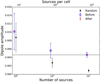Fig. 1. Dipole amplitudes of the quadratic estimator for different sample sizes of purely random skies (black points), skies boosted before pixelisation (blue boxes), and skies boosted after pixelisation (red crosses). The solid line indicates the simulated amplitude d = 4.63 × 10−3. The simulations and the estimations are performed on a HEALPIX grid with resolution Nside = 16.

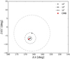Fig. 2. Dipole directions (markers) of the quadratic estimator for different sample sizes of skies boosted after pixelisation, shown in cartesian projection together with the 68% confidence cones (lines). The red dot indicates the simulated dipole direction in equatorial coordinates (RA, Dec) = (167.942, −6.944) deg. The simulations and the estimations are performed on a HEALPIX grid with resolution Nside = 16.

Using possible survey properties from the upcoming Square Kilometre Array (SKA), the estimator of Eq. (26) was already briefly tested with simulations of the cosmic radio dipole (Square Kilometre Array Cosmology Science Working Group 2020; Bengaly et al. 2019). Based on the simulated source counts with 10⁸ to 10⁹ sources, inferred from theoretical power spectra including clustering and evolution, the dipole position (in galactic coordinates) was estimated to have maximal errors of (Δl, Δb)∼(9, 5) deg and with errors on the recovered dipole amplitude of ∼10%.

Over all sample sizes, the recovered position and amplitude of the fiducial kinematic dipole are comparable between boosting before and after the pixelisation. Because of the high difference in computation time, we will opt to boost the source counts directly in subsequent studies. In order to see a percent effect in the source count fluctuations, one has to overcome the shot noise based on the counting process in each cell. By measuring the dipole amplitude in a purely random sample, we can estimate a lower limit of sources necessary to see the fiducial simulated dipole; see Fig. 1.

4.2. Grid and masking effects

To test whether the estimated dipole position is affected by the resolution of the applied grid, we tested the same simulated skies with three different grid resolutions, namely N_side = 16, 32 and 64. The mean spacing of these resolutions between neighbouring cell centres is θ₁₆ = 3.66 deg, θ₃₂ = 1.83 deg, and θ₆₄ = 0.92 deg, with the number of possible directions (cell positions) given as: 3072, 12 288, and 49 152, respectively. In Tables 3 and 4, the estimated dipole directions with errors and offsets to the simulated dipole with d = 0.46 × 10⁻² and d = 1.51 × 10⁻² amplitudes are presented. While using higher resolutions of the position grid, we observe a decreased offset of the estimated dipole direction to the CMB dipole. The error on the estimated dipole direction also decreases slightly with higher resolutions. As the time for one estimation increases together with the resolution, we decided that for further analyses, we would use a position grid with $N_{\mathrm{side}}^{\mathrm{grid}}=32$. For the data we keep a pixelisation resolution of N_side = 16.

Additionally we tested if the quadratic estimator is biased by possible masking procedures. Therefore, we used the boosted skies from the former and applied two different kind of masks to the simulations. Firstly, we tested a galactic cut of equal latitude in steps of five degrees from 5 to 20 deg. The masks are shown in Fig. 3 as red (5 deg), orange (10 deg), green (15 deg), and light blue (20 deg) regions, with the results of the estimations shown in Tables 5 and 6. We observe an increasing positional offset, as well as an increasing positional error when masking larger galactic cuts. The estimated dipole directions with 10⁶ sources is for all masks within two degrees and for 10⁷ sources even below the spacing of the used position grid. For all samples with 10⁶ and 10⁷ sources the estimated dipole amplitudes are in agreement with the simulated kinematic dipole, but increase slightly with increasing galactic cuts.

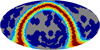Fig. 3. Example masks for different cuts in galactic latitude, with |b| = 5 deg (red), 10 deg (orange), 15 deg (green), and 20 deg (light blue). Additionally, 100 random discs with a radius of 10 deg are masked (blue). The unmasked region is highlighted in grey.

Secondly, we draw random positions on the sky and mask all cells, whose centres are within θ = 10 deg to the random position. We start with one position and increase this masking up to 300 positions, which results in a final fractional sky coverage of f_sky = 0.1. An example of the mask, consisting of 1 out of 100 randomly chosen positions, is also shown in Fig. 3 as the blue regions. We applied the masks to the simulated samples with 10⁶ sources. The estimated dipole amplitude Δd and the difference of the positional offset Δθ to the fiducial dipole as a function of sky coverage f_sky are shown in Figs. 4 and 5. The estimated dipole amplitude (blue solid and red dashed line) with the estimated error (shaded region) in Fig. 4 is, over the complete range of sky coverage, consistent with the simulated kinematic dipole (black line). We observe a varying positional offset (black line) in Fig. 5 from below the mean separation of the position grid to fluctuating offsets between 1.7 deg and 5.5 deg for the example of masking 100 random positions, depending on the simulated dipole amplitude. The shaded regions in Fig. 5 correspond to the 68% and 95% confidence cones of the 300 simulated skies.

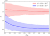Fig. 4. Estimated dipole amplitude for simulated skies with d = 1.51 × 10−2 (dashed line) and d = 0.46 × 10−2 (solid line). The decreasing sky coverage was generated by masking 300 discs with a 10 deg radius at random positions. The fiducial kinematic radio dipole amplitude is shown as a dashed or dotted line, respectively.

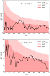Fig. 5. Semi-vertical angles of the 68 and 95% confidence cones (shaded) and the angular offset of the mean direction from the fiducial dipole direction (lines) for d = 1.51 × 10−2 (top) and d = 0.46 × 10−2 (bottom). The decreasing sky coverage was generated by masking 300 discs with 10 deg radius at random positions.

We conclude that the quadratic estimator (26) can reliably distinguish a kinematic dipole of order 10⁻³ from a purely random sky of at least 10⁶ point sources. Depending on the shape of the mask, the positional offsets of the estimated dipole direction are on the order of < 3 deg for cuts of equal galactic latitude or on the order of order 5 deg for unequal masked sky regions.

5. Data

In this work, we used four different radio surveys, namely, the TGSS-ADR1 (Intema et al. 2017), WENSS (Rengelink et al. 1997), SUMSS (Mauch et al. 2003), and NVSS (Condon et al. 1998) to estimate the cosmic radio dipole. The frequency range covered by these four surveys extend over one decade, starting from 147 MHz up to 1.4 GHz. We show the source counts per cell of all four surveys as a HEALPIX map with resolution of N_side = 16 in Fig. 6. The properties of the surveys are summarised in Table 7.

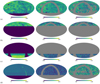Fig. 6. Source counts per HEALPIX cell in equatorial coordinates and Mollweide projection with HEALPIX resolution of Nside = 16. Radio sources observed within the TGSS-ADR1 (a), WENSS (b), SUMSS (c) and NVSS (d) radio source catalogues without flux density threshold are shown in the first column. In the second and third columns, we show the surveys masked with ‘mask d’ and ‘mask n’ and flux density thresholds of 50 mJy (TGSS), 25 mJy (WENSS), 18 mJy (SUMSS), and 25 mJy (NVSS).

5.1. TGSS-ADR1

The first Alternative Data Release of the TIFR GMRT Sky Survey (TGSS-ADR1; Intema et al. 2017) covers the sky between −53 deg and +90 deg declination, which amounts to an area of 36 900 square degrees, or 11.24 sr, resulting in a sky fraction of f_sky ≃ 0.89. It observes the sky with a declination-dependent resolution of 25″ × 25″/cos(Dec − 19 deg) for declinations below 19 deg and at a resolution of 25″ × 25″ for higher declinations. Unfortunately, the observation had problems to resolve certain regions of the sky, which results into a incomplete coverage in a region roughly defined by $6\stackrel{\text{h}}{.}5\le \mathrm{RA}\le 9\stackrel{\text{h}}{.}5$ and 25 deg ≤Dec ≤ 39 deg. In total, the survey observes 640 017 sources at a limiting flux density of 25 mJy with a median rms noise of 3.5 mJy beam⁻¹. The survey is given to be 50% complete at 25 mJy (Intema et al. 2017) and inferred from the plotted completeness function to be 95% at a flux density threshold of 100 mJy. In Fig. 6, the TGSS-ADR1 is shown in a HEALPIX resolution of N_Side = 16, which results in a median source count per cell of $\stackrel{\sim }{n}=221$ and in a sample mean of $\overline{n}=222.32$ with a sample standard deviation of σ = 57.89.

5.2. WENSS

To form the Westerbork Northern Sky Survey (WENSS) with the Westerbork Synthesis Radio Telescope (WSRT), two different catalogues have been compiled at a frequency of 325 MHz (Bremer 1994). These two parts are a main version, which covers the sky from 30 deg to 75 deg declination and a northern pole version, which contains sources above 75 deg declination, while this part was done with a larger bandwidth to decrease the noise level. The resolution of the resulting mosaics is given as 54″ × 54″/sin(Dec) for 325 MHz at FWHM, while the positional accuracy for strong sources is 1.5″.

In a first mini survey of 570 square degrees Rengelink et al. (1997), the survey is estimated to be essentially complete at 30 mJy and by computing the differential source counts to be 50% at 25 mJy. The final catalogue de Bruyn et al. (2000), combined out of the main and polar version, contains a total of 229 420 sources with a limiting flux density of approximately 18 mJy. It covers 10 177 square degrees, or 3.10 sr of the northern sky, which compares to a fractional sky coverage of f_sky = 0.25. In Fig. 6, the sky map of the WENSS survey is shown. We can see that our own galaxy contributes in low counts to the distribution of sources in the sky. We get a mean number of sources per cell of $\overline{n}=265.53$ and a median of $\stackrel{\sim }{n}=286$ with a standard deviation of σ_n = 85.15.

5.3. SUMSS

The final version of the Sydney University Molonglo Sky Survey (SUMSS v2.0; Murphy et al. 2007), which was observed at a central frequency of 843 MHz, contains 210 412 radio sources. The corresponding sky patch of 8100 square degrees, or 2.47 sr has been observed for declinations θ ≤ −30 deg without galactic latitudes of |b| > 10 deg, which sums up to a sky fraction of f_sky = 0.20. The resulting images have a resolution of 45″ × 45″/cos(Dec) with a limiting peak brightness of 6 mJy beam⁻¹ and 10 mJy beam⁻¹, for declinations Dec ≤ −50 deg (southern) and Dec > −50 deg (northern), respectively. In an earlier release (Mauch et al. 2003), of 3500 square degrees and 107 765 radio sources, the two parts were estimated to be complete at 8 mJy and 18 mJy. In order to be complete in both parts of the survey, we applied the same flux density threshold to both parts and make sure it was above 18 mJy.

The source distribution of the final survey is shown in Fig. 6, where the difference between the southern and northern part is clearly visibly by smaller source counts per cell above declinations of −50 deg. The median source count per cell of the complete sample is $\stackrel{\sim }{n}=303$, together with a mean of $\overline{n}=305.43$ and standard deviation of σ = 116.51, which splits up into ${\overline{n}}_s=340.59$ and ${\overline{n}}_n=221.08$ for the southern and northern part, respectively.

5.4. NVSS

The NRAO VLA Sky Survey (NVSS; Condon et al. 1998) observed at a central frequency of 1400 MHz with a bandwidth of 42 MHz covers 33 813 square degree, or 10.3 sr of the full sky, which corresponds to a fraction of sky of about f_sky = 0.82. Covering the sky down to Dec = −40 deg declination the survey contains 1 773 484 sources brighter than 2 mJy peak brightness. The images produced out of this radio survey have a rms noise of 0.45 mJy beam⁻¹ and a resolution at FWHM of 45″. The source catalogue was estimated to be 50% complete at a flux density threshold of 2.5 mJy and 99% complete at 3.4 mJy (Condon et al. 1998). Blake & Wall (2002) pointed out that the NVSS source catalogue still suffers from systematical source density fluctuations below 15 mJy.

In Fig. 6, the map of the full NVSS, with a mean of source counts per cell of $\stackrel{\sim }{n}=691$ and a standard deviation of σ = 120.73 and median of $\overline{n}=684.21$ sources with rejecting cells without sources is shown. It can clearly be seen on the map that our own galaxy contributes in high counts to the distribution. The constant variation in the source counts in the region of the equatorial plane is due to a change in configurations starting at δ ≈ −10 deg and north of it up to δ ≈ +75 deg.

5.5. Masking

All the four surveys are masked with the same strategy, namely, by applying a HEALPIX mask with N_Side = 16 to the source counts per cell. Firstly, we cut the southern hemisphere (or northern in the case of SUMSS) to mask the unobserved regions. The bound is to be set higher or lower to also reject cells, which centres are not below the detection limit, but overlap with their covering area. Secondly we mask the Galactic plane for all surveys with a cut of equal latitude |b| ≤ 10 deg (depending on the cell centre position) in order to account for confusion by the Milky Way.

Additionally we mask unobserved regions, for example in the case of TGSS-ADR1, where failed observations led to a large unobserved region in the north-east. The combination out of these three masks will be used as the default mask, called ‘mask d’. Based on the local rms noise we additionally generate masks defined by the cell averaged local rms noise of all sources in that given cell (σ_b) and denote it ‘mask n’. We use the 68 percentile of the rms maps as the upper bound and reject all cells with higher local noise than the 68% limit. In case of the TGSS and WENSS survey, the local rms noise is directly given in the radio source catalogue. We find for the TGSS ${\sigma }_{\mathrm{b}}^{68}=4.10$ mJy beam⁻¹ and for the WENSS ${\sigma }_{\mathrm{b}}^{68}=4.12$ mJy beam⁻¹. While there is no local rms noise for each source in the NVSS and SUMSS source catalogue available, we adopt the mask defined in Chen & Schwarz (2016). This mask is based on the averaged rms positional uncertainty of sources fainter than 15 mJy in the NVSS, which traces the rms brightness fluctuations σ_b (Condon et al. 1998). For the NVSS, we re-scaled the mask labelled ‘NVSS65’ of Chen & Schwarz (2016) from $N_{\mathrm{side}}=32$ to N_side = 16 and named it ‘mask n’. In the case of the SUMSS survey, we averaged the positional uncertainty per cell relative to the beam size (Chen & Schwarz 2016)

$$\begin{array}{c}\hfill {\sigma }_{\theta }=\sqrt{\frac{{\sigma }_{\varphi }{\sigma }_{\theta }}{{\theta }_{\mathit{FWHM}}^2}sin(\frac{\pi }{2}-\theta )}\end{array}$$(44)

for all sources below the completeness level of S = 18 mJy. From this positional uncertainty per cell, we defined the mask by only using the first 68% of the cells with the limit ${\sigma }_{\theta }^{68}=6.95\times {10}^{-2}$. The full as well as the masked surveys can be seen in Fig. 6, with the full surveys in the left, ‘mask d’ in the middle, and ‘mask n’ in the right column. The reduced sky coverages of the masks are shown in Table 9.

6. Results

6.1. Expected dipole amplitude

Before we estimated the cosmic radio dipole for all four surveys with two different masks and different flux density thresholds, we calculated the expected dipole amplitude based on the source counts of each survey. To each survey, we applied a different flux density threshold. For the TGSS, we used 50, 100, 150, and 200 mJy, the choice of which is motivated by the findings of Rana & Bagla (2019), Dolfi et al. (2019) in the terms of the angular two-point correlation function and of Singal (2019) in terms of the cosmic radio dipole. Motivated by the findings of Rubart & Schwarz (2013), we used the same set of flux density thresholds of 25, 35, 45, and 55 mJy for WENSS, SUMSS and NVSS. For SUMSS and NVSS, we extended the list of thresholds by 18 mJy and 15 mJy, respectively.

As denoted in Eq. (3), the source counts per solid angle and flux density threshold can be defined as a simple power law. In order to fit this power law, we use the least squares method of LMFIT. The results of the fit to the unmasked source counts of the four source catalogues can be seen in Fig. 7 (top). Within 68% confidence intervals we find for the unmasked surveys:

$$\begin{array}{c}\hfill \begin{array}{ccc}& x_{\mathrm{TGSS}}=0.86\pm 0.03,\hfill & \hfill 50\text{mJy}\le S\le 500\text{mJy}\\ \hfill & x_{\mathrm{WENSS}}=0.75\pm 0.03,\hfill & \hfill 25\text{mJy}\le S\le 250\text{mJy}\\ \hfill & x_{\mathrm{SUMSS}}=1.00\pm 0.02,\hfill & \hfill 18\text{mJy}\le S\le 180\text{mJy}\\ \hfill & x_{\mathrm{NVSS}}=1.04\pm 0.02,\hfill & \hfill 15\text{mJy}\le S\le 150\text{mJy}\\ \hfill \end{array}\end{array}$$(45)

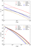Fig. 7. Integral source counts of the TGSS-ADR1, WENSS, SUMSS, and NVSS radio source catalogues, masked with ‘mask d’, as a function of flux density. We fit a function N(> S) ∝ S−x (top) and a more sophisticated function dN/dΩdS ∝ xS−x − κlog10(S/Jy) (bottom) to the counts, which have equal step width in log10(S/Jy). The fitted range depends on the flux threshold of the survey and extends for each survey over one decade.

The lower bound for the fitting range is defined by the smallest flux density threshold that we apply to each survey. The fitting range is then extended over one decade of flux density. We additionally perform the same fit as above, but using the surveys masked with ‘mask d’ and ‘mask n’.

$$\begin{array}{c}\hfill \begin{array}{cc}& \mathrm{mask}d\hfill \\ \hfill & x_{\mathrm{TGSS}}=0.87\pm 0.03\hfill \\ \hfill & x_{\mathrm{WENSS}}=0.76\pm 0.03\hfill \\ \hfill & x_{\mathrm{SUMSS}}=1.00\pm 0.02\hfill \\ \hfill & x_{\mathrm{NVSS}}=1.04\pm 0.02\hfill \\ \hfill \end{array}\begin{array}{cc}& \mathrm{mask}n\hfill \\ \hfill & x_{\mathrm{TGSS}}=0.88\pm 0.03\hfill \\ \hfill & x_{\mathrm{WENSS}}=0.77\pm 0.03\hfill \\ \hfill & x_{\mathrm{SUMSS}}=1.00\pm 0.02\hfill \\ \hfill & x_{\mathrm{NVSS}}=1.05\pm 0.02\hfill \\ \hfill \end{array}\end{array}$$(46)

The fitted slopes of the source counts are consistent between the unmasked and masked surveys, but tend to steepen within error bars with more aggressive masks. These findings are in good agreement with earlier studies, such as Rubart & Schwarz (2013). For NVSS and SUMSS, the results are additionally in good agreement to the usual assumption of x ≈ 1.

Based on the results in Fig. 7 (top), the assumption of a single power law seems unlikely. Tiwari et al. (2015) suggested a deviation from a pure power law, which extends the slope by an extra dependency on the flux density. The improved power law is then defined on the differential source counts as:

$$\begin{array}{c}\hfill \frac{\mathrm{d}N}{\mathrm{d}\mathrm{\Omega }\mathrm{d}S}\propto x{S}^{-1-x-\kappa ln(S/\text{Jy})}.\end{array}$$(47)

The fit of Eq. (47) is carried out in the range from the lowest defined flux density threshold up to 10 Jy. In Fig. 7 (bottom), we show the results of this fit to the differential source of the masked surveys. The resulting best-fit values for x and κ within 68% confidence intervals are:

$$\begin{array}{c}\hfill \begin{array}{cc}& x_{\mathrm{TGSS}}=1.168\pm 0.003,\hfill \\ \hfill & x_{\mathrm{WENSS}}=1.286\pm 0.032,\hfill \\ \hfill & x_{\mathrm{SUMSS}}=1.453\pm 0.022,\hfill \\ \hfill & x_{\mathrm{NVSS}}=1.662\pm 0.014,\hfill \\ \hfill \end{array}\begin{array}{cc}& {\kappa }_{\mathrm{TGSS}}=0.155\pm 0.002\hfill \\ \hfill & {\kappa }_{\mathrm{WENSS}}=0.163\pm 0.008\hfill \\ \hfill & {\kappa }_{\mathrm{SUMSS}}=0.108\pm 0.004\hfill \\ \hfill & {\kappa }_{\mathrm{NVSS}}=0.136\pm 0.003\hfill \\ \hfill \end{array}\end{array}$$(48)

Based on the improved power law of Eq. (47), the expected dipole amplitude can be written as (Tiwari et al. 2015):

$$\begin{array}{c}\hfill d_i=[2+x(1+\alpha )+2\kappa (1+\alpha )\frac{I_2}{I_1}]\beta ,\end{array}$$(49)

with:

$$\begin{array}{cc}\hfill I_1& =x{\displaystyle {\int }_{S_{\lim }}^{10}\mathrm{d}S{S}^{-1-x-\kappa ln(S/\text{Jy})},}\hfill \end{array}$$(50)

$$\begin{array}{cc}\hfill I_2& =x{\displaystyle {\int }_{S_{\lim }}^{10}\mathrm{d}S{S}^{-1-x-\kappa ln(S/\text{Jy})}ln(S/\text{Jy}).}\hfill \end{array}$$(51)

In Table 8, we compare the expected dipole amplitudes from Eqs. (8) and (49). The errors of the best-fit values are propagated to estimate the error of the expected dipole amplitudes. Additionally, we assume the error of the spectral index to be Δα = 0.25 and propagate it accordingly. For WENSS, SUMSS, and NVSS, the expected dipole calculated from the simple fit gives stronger amplitudes than for the improved fit. In the case of TGSS the usual fit gives a significant weaker dipole amplitude compared to the improved fit. The resulting expectations of the simple fit for WENSS and NVSS are also in good agreement to expectations of Rubart & Schwarz (2013), with d_WENSS = (0.42 ± 0.03)×10⁻² and d_NVSS = (0.48 ± 0.04)×10⁻², respectively.

6.2. Measurements of the cosmic radio dipole

The results of the estimation of the cosmic radio dipole from the four different surveys are shown in Table 9. From the estimated dipole direction (ϕ_m, θ_m), we calculated the angular distance Δθ to the fiducial kinematic dipole (ϕ_f, θ_f) of the CMB (see Sect. 2) using Eq. (43). The errors of each estimation are computed from 100 bootstraps of the source counts map. Additionally we add half the cell size of the position grid to the estimated error in order to account for the discretisation. In our case, we used a position grid of N_side = 32 resolution, so cells have a mean spacing of Δθ = 1.83 deg. The directional offset error was computed by taking the standard deviation of the directional offsets from the dipole boosted skies of the surveys:

$$\begin{array}{c}\hfill {\sigma }_{\mathrm{\Delta }\theta }={\displaystyle \sqrt{\frac{1}{N}\sum _i^N{(\mathrm{\Delta }{\theta }_i-\mathrm{\Delta }{\theta }_{\mathrm{obs}})}^2}.}\end{array}$$(52)

We observed consistent dipole directions and dipole amplitudes for each survey between the two different masking strategies. We find a good self-consistency for the dipole amplitude between the estimates from WENSS and SUMSS. For the NVSS, we find smaller dipole amplitudes than for WENSS and SUMSS, but they are consistent within one to two sigma. The estimated dipole amplitude for the TGSS shows a significant excess by a factor of two to three in comparison to the other surveys. In general, all four surveys show an increased dipole amplitude, as well as a directional offset compared to the kinematic CMB dipole. Based on the χ²/d.o.f., we find the best agreement of the dipole modulation to the observed source counts for the NVSS catalogue. Additionally, the smallest amplitude is found for NVSS with a flux density threshold of 15 mJy and masked with ‘mask n’. On the other hand, the smallest directional offset to the CMB dipole of 1.54 deg is found for NVSS with 45 mJy and ‘mask n’. The estimated dipole direction of SUMSS shows the largest offsets from the kinematic CMB dipole direction, which is mainly driven by the values in right ascension. The estimated declination remains in good agreement with the CMB. In most cases, the uncertainties of the dipole direction directly increase with a decreasing number of sources and decreasing dipole amplitude. The former was expected based on the testing process described in Sect. 4. Driven by the large dipole amplitude found for the TGSS, we observe relatively small errors for the estimated right ascension and declination as compared to the results from the other surveys. The results of the cosmic radio dipole found in the TGSS, WENSS, and NVSS are in good agreement with the results from the literature. A detailed list of earlier results from several studies is presented in Appendix A.

The excess of the dipole amplitude found in the TGSS, as compared to other surveys, is withina two-sigma agreement to results of Bengaly et al. (2018) and Singal (2019); for more, see Table A.3. As the TGSS is reported to be incomplete below 100 mJy, the smallest flux density threshold in our TGSS samples shows the largest offset to the CMB dipole direction. Among the ‘mask d’ samples, the incomplete sample additionally shows the largest dipole amplitude. The three other flux density threshold samples show a self-consistent dipole amplitude and dipole direction. The ‘mask n’ results show a slightly increased directional offset and slightly increased dipole amplitude, but they are nonetheless self-consistent. Based on the χ²/d.o.f., the agreement of the dipole hypothesis to the data improves continuously for increasing flux density thresholds. The faintest TGSS samples of both masks show a significantly lager χ²/d.o.f. than higher flux density thresholds.

In general, all our measured amplitudes of the WENSS ‘mask d’ and ‘mask n’ samples are consistent within one sigma. For the faintest samples, however, we find the largest dipole amplitude, which decreases slightly for higher flux density thresholds. The results of our WENSS samples are also in good agreement to the results reported in Rubart & Schwarz (2013), as shown in Table A.2, which were obtained using a linear estimator. The increasing offset of the dipole direction in the WENSS samples is mostly driven by the measured right ascension angles. We observe a decreasing right ascension for higher flux density thresholds and a with the CMB dipole direction consistent declination. Similar to the TGSS, we find an improved fit of the dipole modulation for increasing flux density thresholds. The strongest improvement, based on the χ²/d.o.f., we observe between the 25 and 35 mJy flux density thresholds for both masks.

For the SUMSS 18 mJy sample with both masks we also observe the largest amplitude across the flux density thresholds. The measured amplitudes for the higher flux densities display a good consistency, but they decrease with an increasing flux density threshold. The declination of all SUMSS samples is consistent with the CMB dipole. The right ascension, however, shows a clear offset and is inconsistent within three sigma with the right ascension of the CMB dipole direction. We ensured that our measurements in the SUMSS samples are not biased towards a overdense cell in the south east, which is also not masked by ‘mask n’. We manually masked this cell and measured a dipole of 2.9 × 10⁻³ towards (104.06, +3.58) deg for S > 25 mJy and ‘mask d’, or 3.1 × 10⁻³ towards (102.66, 0.00) deg for S > 25 mJy and ‘mask n’, which is consistent with the previous results. Alongside these previous results, we also find the largest χ²/d.o.f. for the second flux density threshold of both masks. The faintest samples, contrary to those of TGSS and WENSS, show higher flux density thresholds that are consistent with the test statistics.

The dipole amplitude results from the NVSS samples shows nearly consistently the smallest values and are self-consistent for both masks. Beside the amplitudes reported in Blake & Wall (2002), we find good agreement to the measured dipole amplitudes of Singal (2011), Rubart & Schwarz (2013), Bengaly et al. (2018) and Tiwari & Nusser (2016). For a detailed list on results from the NVSS see Table A.1. The measured dipole direction are in good agreement to earlier results, except for the measured direction from Gibelyou & Huterer (2012). Between the two masks, we find the smallest offsets to the CMB dipole direction for ‘mask n’ and in detail for a flux density threshold of 45 mJy. The directional offsets of ‘mask d’ are in good agreement to the offsets observed for the WENSS with 25 and 35 mJy flux density threshold. The agreement of the dipole modulation to the observed source counts is consistent for values greater than 15 mJy. For the 15 mJy flux density threshold of both masks, we find within the NVSS samples the poorest fit, which is in good agreement with the previously observed systematical source density fluctuations below 15 mJy (Blake & Wall 2002).

In general, the measurements from samples below, or close to completeness, such as TGSS 50 mJy, WENSS 25 mJy, and SUMSS 18 mJy show inconsistent results when compared to samples with flux density thresholds above completeness. Therefore, we focus on samples with higher flux densities in the conclusion.

6.3. TGSS and NVSS cross-matched catalogue

To investigate the strong difference in the estimated dipole amplitude between the TGSS-ADR1 and NVSS survey, we cross-matched both catalogues and named it TGSSxNVSS. The cross-matching was done with TOPCAT (Taylor 2005), where the NVSS sources are matched within 10″ to the TGSS sources. We generated a catalogue for all 519 414 cross-matched sources consisting out of TGSS and NVSS source positions, as well as flux densities at 147.5 MHz and 1.4 GHz. To mask the cross-matched catalogue properly, we combine both ‘mask d’ of the NVSS and TGSS survey. The masked source counts per cell of the TGSSxNVSS catalogue can be seen in Fig. 8 (top), with 417 840 sources after masking. We additionally show the distribution of both flux densities in Fig. 8 (bottom), where the NVSS flux densities have been scaled to TGSS frequency by α = 0.75. By eye, the HEALPIX map of the TGSSxNVSS and TGSS (Fig. 6) catalogue show a similar source counts distribution across the sky and are not comparable to the homogenous source distribution of the NVSS. The flux density distribution of the TGSS flux densities of the TGSSxNVSS show a stronger peak and narrower distribution than the scaled flux densities of the NVSS.

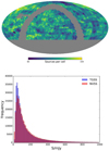Fig. 8. Masked source counts per cell of the cross matched TGSSxNVSS catalogue (top) and flux density distribution of the cross matched sources of the TGSS and NVSS survey (bottom). The flux densities of the NVSS survey have been scaled by α = 0.75.

We estimate the cosmic radio dipole of the masked TGSSxNVSS catalogue without flux density threshold and show the result in Table 10. The resulting dipole amplitude for the full TGSSxNVSS sample is the upper boundary of the assumed amplitude range in the χ² minimisation. Based on the large χ²/d.o.f. in comparison to results from the former, we assume that a dipole modulation is not preferred by this sample. As the cross-matching does not guaranty the completeness of the sample, we apply a flux density threshold to either the flux densities of the TGSS, or of the NVSS sources. To have a similar flux density threshold in both cases, we scale the 25 mJy flux density threshold of the NVSS sample using α = 0.75 to the frequency of the TGSS, which is 135 mJy. Applying these flux density thresholds to either the TGSS or the NVSS flux densities of the cross-matched sources we find two dipole amplitudes, which strongly differ from each other. The higher dipole amplitude and also dipole direction, measured for the TGSSx flux density threshold is comparable to the dipole measured for the full TGSS sample of Sect. 6.2. The same holds true for the xNVSS dipole measurement when compared to the full NVSS sample. This suggest that the sources of both samples follow a different flux density distribution. The χ²/d.o.f. values of both flux density threshold samples shows a clearly improved fit of the dipole to the data than for the full TGSSxNVSS sample. Both values are in good agreement to the corresponding samples of the original surveys, with a slight indication for a better fit in both cases. Out of the 159 240 sources of the TGSSx flux density threshold sample 139 161 sources are the same in the xNVSS flux density threshold sample, which has 176 433 sources initially. We again estimate the dipole of this common flux density threshold sample and find a dipole amplitude in between the two amplitudes of the previous results. The resulting dipole direction is in agreement with previous findings.

7. Discussion

We investigated the possible biases of a simple linear estimator (Crawford 2009), which was used in the literature to estimate the cosmic radio dipole (e.g. Singal 2011, 2019; Rubart & Schwarz 2013). Our detailed analysis demonstrates the limited application of such an estimator due to the directional biases introduced by the masking procedure. Possible biases affecting the estimated dipole amplitude have already been discussed in Rubart & Schwarz (2013).

Therefore, we analysed a quadratic estimator, based on a χ² minimisation, which uses source counts in equal area cells to determine the cosmic radio dipole. The quadratic estimator is tested against possible contributions from masking and resolution dependencies. We conclude that the quadratic estimator, which was already briefly discussed in a cosmic radio dipole forecast of the SKA (Bengaly et al. 2019; Square Kilometre Array Cosmology Science Working Group 2020), is suitable for distinguishing a simulated kinematic dipole at a percent level from contributions of a purely random sky. The recovered position of a simulated kinematic dipole can securely be estimated with positional offsets of 1.4 deg or 0.7 deg, for full skies with 10⁶ or 10⁷ simulated sources. These offsets are already below the mean separation of the cells used for the pixelisation of the sky, which is 3.66 deg. Increasing the resolution of the search-grid for the dipole direction does not significantly improve the estimation, as it is limited by the cell size of the data. The amplitude can be recovered with uncertainties of ∼10% for 10⁷ simulated sources. A kinematic dipole with a higher amplitude is detectable for even smaller source densities.

We discussed two possible masking strategies. For cuts of equal galactic latitude, we found no significant effect on the recovered dipole direction and amplitude. Masking randomly regions of the simulated sky with 10⁶ sources can increase the directional offset from ∼1.4 deg to ∼5.5 deg. The recovered dipole amplitude seems to be less affected.

We applied the quadratic estimator to the TGSS-ADR1, WENSS, SUMSS, and NVSS radio source catalogues. In general we find self-consistency for the estimated dipole amplitude and direction between two different masking strategies in each survey. Rejecting regions with higher noise flux densities or larger positional uncertainties improves the quality of the fit, but does not significantly change the resulting cosmic radio dipole. Comparing our measured dipole directions and amplitudes to other published results of the TGSS (Bengaly et al. 2018), WENSS (Rubart & Schwarz 2013) and NVSS (e.g., Blake & Wall 2002; Singal 2011; Rubart & Schwarz 2013) displays a good agreement. The dipole amplitude, inferred from the SUMSS survey, is consistent with the results from WENSS and NVSS, but shows a larger directional offset. For a combined catalogue of NVSS and SUMSS sources (NVSUMSS), Colin et al. (2017) found a dipole with velocity of 1729 ± 187 km s⁻¹ towards (RA, Dec) = (149 ± 2, −17 ± 12) deg, which is in agreement with the results of the NVSS. We find the best agreement of a dipole modulation to the observed source counts, based on the test statistic χ²/d.o.f., for the NVSS survey. The excess of the measured dipole amplitude from WENSS and NVSS compared to the CMB still persists and increases even more for the TGSS. Comparing the results of NVSS dipole to the (kinematic) dipole of the CMB, we find an increased amplitude by a factor of three to four. Contrariwise, for the more aggressive ‘mask n’, the estimated dipole direction is in good agreement to the dipole direction of the CMB. For the TGSS, the dipole amplitude increases by an additional factor of three to four, while compared to the NVSS.

In order to compare the observed dipole amplitudes of each survey to the CMB dipole, we simulate source count maps, which include the CMB dipole, the effect of limited number of sources, and reduced sky coverage. The recovered simulated dipole amplitudes are shown in Fig. 9 with open symbols. We observe, for the TGSS-ADR1 and NVSS, a clear discrepancy between the simulated CMB dipole amplitude and the observed dipole amplitude. Therefore, the contributions mentioned above are not sufficient to explain the increased dipole amplitude with respect to the CMB dipole. On the other hand, for the WENSS and SUMSS source catalogues, the effects of a low number of sources and a decreased sky coverage could explain at least a sizable fraction of the observed excess.

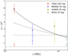Fig. 9. Comparison of dipole amplitudes observed at different frequencies for the TGSS-ADR1, WENSS, SUMSS, and NVSS masked with ‘mask d’. A function f(ν) = A(ν/1 GHz)m is fitted to the dipole amplitudes (solid lines), which results in A = (2.16 ± 0.53)×10−2 and m = −0.51 ± 0.15 with χ2/d.o.f. = 1.23. Results of a power law and constant dipole amplitude fit excluding the TGSS are shown as dashed-dotted and dotted lines, respectively. Simulations for each survey coverage with the CMB dipole (dashed line) are shown as open symbols.

To investigate the difference between the TGSS and NVSS further, we measured the dipole for a common sub-sample. Also in the cross-matched catalogue the TGSS-ADR1 dipole amplitude is significantly larger than the NVSS dipole amplitude. We also created a common sub-sample of the TGSSxNVSS catalogue, by scaling the NVSS flux density threshold to the TGSS frequency. For this sub-sample, we find a intermediate dipole amplitude. Already for the single flux density thresholds, applied either to the TGSS or NVSS flux densities, improves the agreement of the dipole modulation to the observed source counts. Based on the cross-matched catalogue of TGSS and NVSS sources, we can conclude that the observed dipole amplitudes of these two surveys are real.

The difference in the dipole amplitudes of the analysed surveys can not be explained by different slopes of the number counts, as shown in Sect. 6.1. Therefore, we suggest a frequency dependence of the cosmic radio dipole, which is also present in the cross-matched catalogue. In order to quantify the dependence of the dipole amplitude on the frequency, we fitted a function of the form f(ν) = A(ν/1 GHz)^m to the dipole amplitudes (see Fig. 9). For the fitting, we used the python package LMFIT (Newville et al. 2016) with the default Levenberg-Marquardt least-square minimisation. We chose the dipole amplitudes from our set of analysed flux density thresholds, such that they are roughly comparable to a flux density threshold scaled from 25 mJy at 1.4 GHz to the corresponding frequency. For the dipole amplitudes of ‘mask d’, we find A = (2.16 ± 0.53)×10⁻² and m = −0.51 ± 0.15 with χ²/d.o.f. = 1.23 (see Fig. 9 solid line). Masking with ‘mask n’ results in a slightly steepened dependency, with A = (1.98 ± 0.55)×10⁻², m = −0.61 ± 0.16, and χ²/d.o.f. = 1.25.

Excluding the TGSS result form the fit, we still find a power law in agreement with the previous fit (Fig. 9 dashed-dotted line), but fitting a constant to the WENSS, SUMSS, and NVSS dipole amplitudes alone provides an equally good fit (Fig. 9 dotted line). Therefore, we cannot exclude that the observed frequency dependence might be linked to issues with the flux density calibration of the TGSS (see the discussion below), but we see a self-consistent trend across all frequencies.

This is also supported by a fit to dipole results of the cross-matched catalogue (see Fig. 10). We find A = (2.67 ± 0.70)×10⁻² together with m = −0.47 ± 0.16. In this analysis, the dipole result of the common flux density threshold sample of the TGSSxNVSS catalogue was assigned to the geometric mean frequency of the TGSS and NVSS frequencies. As shown above (Table 8), a radio dipole dominated by the kinematic effect is not expected to show such a prominent dependence on frequency.

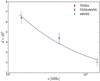Fig. 10. Comparison of dipole amplitudes from the cross-matched TGSSxNVSS catalogue. For the common flux density threshold sample of TGSSxNVSS, the geometric mean was used to determine the frequency. A linear function f(ν) = A(ν/1 GHz)m is fitted to the dipole amplitudes (solid line), which results in A = (2.67 ± 0.70)×10−2 and m = −0.47 ± 0.16, with χ2/d.o.f. = 1.44.

Several aspects on the dipole amplitude and direction have already been investigated in previous studies. Rubart et al. (2014) investigated the contribution of spherically symmetric local structures to the measured dipole of a linear estimator. By simulating a single void, while the observer is sitting at the edge of the void with radius R_v = 0.07R_H (R_H Hubble distance), they found a dipole contribution of d_void = (0.21 ± 0.01)×10⁻² for the linear estimator of Rubart & Schwarz (2013). Varying the void parameters can increase the dipole contribution, but with just one void, it cannot fully explain the discrepancy between the CMB and the radio dipole. Increasing the number of voids, or in general over- and under-densities would add up the contribution to the observed dipole amplitude. Additionally, it has been shown that such an contribution would depend on the frequency of the surveys. In general the contribution from structures in the line of sight can relax the difference between the CMB and the radio dipole, observed, for instance, with the NVSS. But in order to fully explain the large discrepancy between the NVSS and TGSS dipole, we would need unrealistically huge structures. Contributions from local structure and superclusters to the cosmic radio dipole have been investigated by Colin et al. (2017) and appear to have an insignificant influence on the measured large-scale dipole found in NVSS and NVSUMSS.

In a forecast of possible measurements with the upcoming SKA, Bengaly et al. (2019) simulated number count maps for the SKA survey specifications in Phase 1 and 2. They found a increasing contribution from local structures with increasing flux density threshold. Removing sources with z ≤ 0.1 from the simulations in Bengaly et al. (2019) improved the results most effectively and in good agreement with the results from Tiwari & Nusser (2016). Additional contributions, such as bulk flows, are also expected to contribute to the cosmic radio dipole.

Systematical effects, such as a large-scale flux density offset for the TGSS-ADR1 compared to the GaLactic and Extragalactic All-sky Murchison Widefield Array (GLEAM; Hurley-Walker et al. 2017), have been found by Tiwari et al. (2019). The flux density offsets are likely to contribute to the dipole and other large-scale source density measurements. While measuring the power spectrum of the TGSS-ADR1, Tiwari et al. (2019) found a dipole of |D| = 0.05 at S > 100 mJy, which is slightly smaller than previous results from Bengaly et al. (2018) and our own results.

Further distinctions between contributions from large structures or artefacts in the survey are necessary to reveal the real nature of the cosmic radio dipole. To better distinguish contributions from local structure and shot noise effects with the quadratic estimator, a higher source density is needed. Upcoming surveys, such as further data releases of the LOFAR two-metre sky survey (LoTSS; Shimwell et al. 2017), which is carried out with the LOw Frequency ARray (LOFAR; van Haarlem et al. 2013), will eventually cover a large enough sky fraction to measure the cosmic radio dipole with a much higher precision. With follow-up studies, such as the WEAVE-LOFAR survey (Smith et al. 2016), using the William Herschel Telescope Enhanced Area Velocity Explorer (WEAVE; Dalton et al. 2012, 2014), it will be possible to measure spectroscopic redshifts for a subsample of the LoTSS survey. As pointed out previously, forecast in terms of the SKA showed the possibility to measure the cosmic radio dipole with ∼10% accuracy (Square Kilometre Array Cosmology Science Working Group 2020; Bengaly et al. 2019). Additionally, the Evolutionary Map of the Universe (EMU; Norris et al. 2011) will eventually map the entire southern sky at a frequency of 1.3 GHz and is expected to detect ∼70 million radio sources. The field of view of EMU will fully cover the Dark Energy Survey (DES; The Dark Energy Survey Collaboration 2005), which will provide photometric redshifts of optical counterparts. Cross-matching new radio surveys with existing optical and infrared surveys will help to distinguish contributions from local structure to the observed cosmic radio dipole. In upcoming surveys, we expect contributions from local structure to show a similar frequency dependence, as shown in this study for the surveys analysed.

8. Conclusions

In summary, we analysed the efficacy of a quadratic estimator for the cosmic radio dipole, which appears to be unbiased with respect to masking. With this quadratic estimator, we can recover estimates of the cosmic radio dipole for the NVSS, WENSS, and TGSS from the literature. In addition, for the first time, we were able to produce a dipole estimation for the SUMSS catalogue.

For all analysed surveys, we observe an excess in the dipole amplitude with respect to the expected results, derived from the CMB dipole. The dipole direction is consistent with the direction of the CMB dipole. This results are in agreement with various other studies (e.g., Blake & Wall 2002; Singal 2011; Rubart & Schwarz 2013). Different estimators and masking strategies do not change this result. We also find a frequency dependence on the part of the observed cosmic radio dipole, which is incompatible with a kinematic effect that is expected to be (almost) achromatic. However, dropping the lowest frequency survey from the analysis would allow for a frequency-independent dipole amplitude, however, its amplitude would then be in conflict with the observed CMB dipole.

Upcoming telescopes and surveys, such as the Square Kilometre Array, the Evolutionary Map of the Universe, and the LOFAR two-metre sky survey and their higher sensitivities, will hopefully help improve the understanding of the discrepancy between the CMB and the cosmic radio dipole. In a next step, we plan a radio continuum survey complemented with photometric redshifts, such as LoTSS, which will allow us to test whether nearby cosmic structures could be held responsible for the observed signal and its frequency dependence.

Acknowledgments

This research made use of Astropy, a community-developed core Python package for astronomy (Astropy Collaboration 2013) hosted at http://www.astropy.org/, and of the astropy-based reproject package (http://reproject.readthedocs.io/en/stable/). Some of the results in this paper have been derived using the healpy (Zonca et al. 2019) and HEALPix (Górski et al. 2005) package. This research made use of TOPCAT (Taylor 2005), matplotlib (Hunter 2007), NumPy (Walt et al. 2011), lmfit (Newville et al. 2016) and SciPy (Virtanen et al. 2020). We thank the staff of the GMRT that made these observations possible. GMRT is run by the National Centre for Radio Astrophysics of the Tata Institute of Fundamental Research. TMS and DJS acknowledge the Research Training Group 1620 ‘Models of Gravity’, supported by Deutsche Forschungsgemeinschaft (DFG) and by the German Federal Ministry for Science and Research BMBF-Verbundforschungsprojekt D-LOFAR IV (grant number 05A17PBA). MSR acknowledges financial support from the Friedrich-Ebert-Stiftung.

References

Appendix A: Earlier results

In Tables A.1–A.3, we compare the results of the cosmic radio dipole for the NVSS, WENSS, and TGSS-ADR1 radio source catalogues. The results have been derived from different approaches and estimators, which are shortly presented in the following.

Rubart & Schwarz (2013) use a three dimensional linear estimator (linear 3D), introduced by Crawford (2009):

$$\begin{array}{c}\hfill R_{3\mathrm{D}}={\displaystyle \sum _i^N{\widehat{r}}_i,}\end{array}$$(A.1)

which points towards the main anisotropy of the source distribution with sources at position r_i. As the masking affects the measured dipole amplitude, they correct the estimated dipole amplitude $d=|\frac{3}{N}{R}_{3\mathrm{D}}|$ as:

$$\begin{array}{c}\hfill {⟨d_{3\mathrm{D}}⟩}_{\text{mask}}=\sqrt{k_{3\mathrm{D}}^2{d}^2+\frac{9}{N^2}⟨R_{3\mathrm{D}}^{\text{random}}⟩},\end{array}$$(A.2)

with a correction factor estimated from simulations with a given dipole:

$$\begin{array}{c}\hfill k=\sqrt{{\stackrel{\sim }{k}}^2+\frac{9{⟨R^{\mathrm{Random}}⟩}^2}{d^2{N}^2}({\stackrel{\sim }{k}}^2-1)}.\end{array}$$(A.3)

Due to a directional bias in the declination, Rubart & Schwarz (2013) introduced in the same work a two-dimensional estimator (linear 2DCG):

$$\begin{array}{c}\hfill R_{2\mathrm{D}}={\displaystyle \sum _i^N\left(\begin{array}{c}cos{\phi }_{i}sin{\vartheta }_i\\ sin{\phi }_{i}sin{\vartheta }_i\\ 0\end{array}\right),}\end{array}$$(A.4)

with a masking correction for the dipole amplitude:

$$\begin{array}{c}\hfill {⟨d_{2\mathrm{D}}⟩}_{\text{mask}}=\sqrt{k_{2\mathrm{D}}^2{d}^2{sin}^2{\vartheta }_d+\frac{9}{N^2}{⟨R^{{\text{random}}_{2\mathrm{D}}}⟩}^2}.\end{array}$$(A.5)

Singal (2011, 2019) uses the same three-dimensional estimator (Eq. (A.1)) to estimate the direction of the dipole, while the dipole amplitude is estimated via the difference of the source counts:

$$\begin{array}{c}\hfill d=\frac{3}{2k}\frac{\mathrm{\Delta }N}{N}=\frac{3}{2k}\frac{\sum cos{\theta }_i}{\sum |cos{\theta }_i|},\end{array}$$(A.6)

with θ_i the polar angle between the ith source and the dipole direction, and a numerical computed correction factor k. Similarly, Singal (2011, 2019) uses the flux density to define a ‘sky brightness’ estimator for the dipole direction:

$$\begin{array}{c}\hfill R={\displaystyle \sum _i^N{S}_i{\widehat{r}}_i.}\end{array}$$(A.7)

The dipole amplitude can then be estimated via:

$$\begin{array}{c}\hfill d=\frac{3}{2k}\frac{\mathrm{\Delta }F}{F}=\frac{3}{2k}\frac{\sum S_{i}cos{\theta }_i}{\sum S_i|cos{\theta }_i|}.\end{array}$$(A.8)

Gibelyou & Huterer (2012) compares HEALPIX source count maps to maps of randomly chosen directions in order to find the dipole direction via:

$$\begin{array}{c}\hfill R_{3\mathrm{DM}}={\displaystyle \sum _i^{N_D}\widehat{r_i}-\frac{N_{\mathrm{D}}}{N_{\mathrm{R}}}\sum _j^{N_{\mathrm{R}}}\widehat{r_j}·}\end{array}$$(A.9)

The dipole amplitude is then estimated from the likelihood function marginalised over all directions.

Based on a HEALPIX source count map, Tiwari & Nusser (2016) convert the density contrast:

$$\begin{array}{c}\hfill \mathrm{\Delta }(\widehat{r})=\frac{N(\widehat{r})}{\overline{N}}-1\end{array}$$(A.10)

into spherical harmonics:

$$\begin{array}{c}\hfill \mathrm{\Delta }(\widehat{r})={\displaystyle \sum _{l=1}^{\infty }\sum _{m=-l}^{+l}{a}_{\mathit{lm}}{Y}_{\mathit{lm}}(\widehat{r}),}\end{array}$$(A.11)

$$\begin{array}{c}\hfill a_{\mathit{lm}}={{\displaystyle \int }}_{4\pi }\mathrm{d}\mathrm{\Omega }\mathrm{\Delta }(\widehat{r})Y_{\mathit{lm}}(\widehat{r}).\end{array}$$(A.12)

Using the observed power spectrum:

$$\begin{array}{c}\hfill C_l^{\mathrm{obs}}=\frac{⟨|a_{\mathit{lm}}{|}^2⟩}{J_{\mathit{lm}}}-\frac{1}{\overline{N}},\end{array}$$(A.13)

of the observed density contrast, with a correction for the survey coverage:

$$\begin{array}{c}\hfill J_{\mathit{lm}}={\displaystyle {\int }_{\mathrm{survey}}}\mathrm{d}\mathrm{\Omega }{|Y_{\mathit{lm}}|}^2,\end{array}$$(A.14)

they compute the dipole amplitude as:

$$\begin{array}{c}\hfill C_1^{\mathrm{obs}}=\frac{4\pi }{9}{d}^2.\end{array}$$(A.15)

Due to the incomplete sky coverage, Blake & Wall (2002) measured moments 1 ≤ l ≤ 3 of the spherical harmonics. In their work, the dipole amplitude and direction are estimated by varying both on a given grid and compare them to the observed harmonic coefficients:

$$\begin{array}{c}\hfill a_{l,m}={\displaystyle \sum _{i=1}^N{Y}_{l,m}^{\ast }({\vartheta }_i,{\phi }_i).}\end{array}$$(A.16)

Another approach to using the source counts defined by a HEALP IX map was investigated by Bengaly et al. (2018). They split the sky into hemispheres and calculated the source count difference of opposite hemispheres via:

$$\begin{array}{c}\hfill \mathrm{\Delta }(\theta )=\frac{{\sigma }_i^{\mathrm{U}}(\theta )-{\sigma }_i^{\mathrm{D}}(\theta )}{\sigma }=d_{\mathrm{obs}}cos\theta ,\end{array}$$(A.17)

with θ the separation of the estimated direction to the ith pixel and the source density of the ‘up’ (U) or ‘down’ (D) hemispheres:

$$\begin{array}{c}\hfill {\sigma }_i=\frac{N_i}{2\pi {(f_{\mathrm{sky}})}_i}·\end{array}$$(A.18)

All Tables

All Figures

	Fig. 1. Dipole amplitudes of the quadratic estimator for different sample sizes of purely random skies (black points), skies boosted before pixelisation (blue boxes), and skies boosted after pixelisation (red crosses). The solid line indicates the simulated amplitude d = 4.63 × 10−3. The simulations and the estimations are performed on a HEALPIX grid with resolution Nside = 16.
In the text

Fig. 2. Dipole directions (markers) of the quadratic estimator for different sample sizes of skies boosted after pixelisation, shown in cartesian projection together with the 68% confidence cones (lines). The red dot indicates the simulated dipole direction in equatorial coordinates (RA, Dec) = (167.942, −6.944) deg. The simulations and the estimations are performed on a HEALPIX grid with resolution Nside = 16.

In the text

	Fig. 3. Example masks for different cuts in galactic latitude, with |b| = 5 deg (red), 10 deg (orange), 15 deg (green), and 20 deg (light blue). Additionally, 100 random discs with a radius of 10 deg are masked (blue). The unmasked region is highlighted in grey.
In the text

	Fig. 4. Estimated dipole amplitude for simulated skies with d = 1.51 × 10−2 (dashed line) and d = 0.46 × 10−2 (solid line). The decreasing sky coverage was generated by masking 300 discs with a 10 deg radius at random positions. The fiducial kinematic radio dipole amplitude is shown as a dashed or dotted line, respectively.
In the text

	Fig. 5. Semi-vertical angles of the 68 and 95% confidence cones (shaded) and the angular offset of the mean direction from the fiducial dipole direction (lines) for d = 1.51 × 10−2 (top) and d = 0.46 × 10−2 (bottom). The decreasing sky coverage was generated by masking 300 discs with 10 deg radius at random positions.
In the text

Fig. 6. Source counts per HEALPIX cell in equatorial coordinates and Mollweide projection with HEALPIX resolution of Nside = 16. Radio sources observed within the TGSS-ADR1 (a), WENSS (b), SUMSS (c) and NVSS (d) radio source catalogues without flux density threshold are shown in the first column. In the second and third columns, we show the surveys masked with ‘mask d’ and ‘mask n’ and flux density thresholds of 50 mJy (TGSS), 25 mJy (WENSS), 18 mJy (SUMSS), and 25 mJy (NVSS).

In the text

Fig. 7. Integral source counts of the TGSS-ADR1, WENSS, SUMSS, and NVSS radio source catalogues, masked with ‘mask d’, as a function of flux density. We fit a function N(> S) ∝ S−x (top) and a more sophisticated function dN/dΩdS ∝ xS−x − κlog10(S/Jy) (bottom) to the counts, which have equal step width in log10(S/Jy). The fitted range depends on the flux threshold of the survey and extends for each survey over one decade.

In the text

	Fig. 8. Masked source counts per cell of the cross matched TGSSxNVSS catalogue (top) and flux density distribution of the cross matched sources of the TGSS and NVSS survey (bottom). The flux densities of the NVSS survey have been scaled by α = 0.75.
In the text

Fig. 9. Comparison of dipole amplitudes observed at different frequencies for the TGSS-ADR1, WENSS, SUMSS, and NVSS masked with ‘mask d’. A function f(ν) = A(ν/1 GHz)m is fitted to the dipole amplitudes (solid lines), which results in A = (2.16 ± 0.53)×10−2 and m = −0.51 ± 0.15 with χ2/d.o.f. = 1.23. Results of a power law and constant dipole amplitude fit excluding the TGSS are shown as dashed-dotted and dotted lines, respectively. Simulations for each survey coverage with the CMB dipole (dashed line) are shown as open symbols.

In the text

	Fig. 10. Comparison of dipole amplitudes from the cross-matched TGSSxNVSS catalogue. For the common flux density threshold sample of TGSSxNVSS, the geometric mean was used to determine the frequency. A linear function f(ν) = A(ν/1 GHz)m is fitted to the dipole amplitudes (solid line), which results in A = (2.67 ± 0.70)×10−2 and m = −0.47 ± 0.16, with χ2/d.o.f. = 1.44.
In the text

References

- Astropy Collaboration (Robitaille, T. P., et al.) 2013, A&A, 558, A33 [NASA ADS] [CrossRef] [EDP Sciences] [Google Scholar]
- Bengaly, C. A. P., Maartens, R., & Santos, M. G. 2018, JCAP, 2018, 031 [Google Scholar]
- Bengaly, C. A. P., Siewert, T. M., Schwarz, D. J., & Maartens, R. 2019, MNRAS, 486, 1350 [NASA ADS] [CrossRef] [Google Scholar]
- Blake, C., & Wall, J. 2002, Nature, 416, 150 [NASA ADS] [CrossRef] [Google Scholar]
- Bremer, M. A. R. 1994, in The Westerbork Northern Sky Survey (WENSS:) A Radio Survey Using the Mosaicing Technique, eds. D. R. Crabtree, R. J. Hanisch, & J. Barnes, ASP Conf. Ser., 61, 175 [NASA ADS] [Google Scholar]
- Chen, S., & Schwarz, D. J. 2016, A&A, 591, A135 [NASA ADS] [CrossRef] [EDP Sciences] [Google Scholar]
- Colin, J., Mohayaee, R., Rameez, M., & Sarkar, S. 2017, MNRAS, 471, 1045 [NASA ADS] [CrossRef] [Google Scholar]
- Condon, J. J., Cotton, W. D., Greisen, E. W., et al. 1998, AJ, 115, 1693 [NASA ADS] [CrossRef] [Google Scholar]
- Crawford, F. 2009, ApJ, 692, 887 [NASA ADS] [CrossRef] [Google Scholar]
- Dalton, G., Trager, S. C., Abrams, D. C., et al. 2012, in Ground-based and Airborne Instrumentation for Astronomy IV, SPIE Conf. Ser., 8446, 84460P [NASA ADS] [Google Scholar]
- Dalton, G., Trager, S., Abrams, D. C., et al. 2014, in Ground-based and Airborne Instrumentation for Astronomy V, SPIE Conf. Ser., 9147, 91470L [Google Scholar]
- de Bruyn, G., Miley, G., Rengelink, R., et al. 2000, VizieR Online Data Catalog: VIII/62 [Google Scholar]
- de Gasperin, F., Intema, H. T., & Frail, D. A. 2018, MNRAS, 474, 5008 [NASA ADS] [CrossRef] [Google Scholar]
- Dolfi, A., Branchini, E., Bilicki, M., et al. 2019, A&A, 623, A148 [CrossRef] [EDP Sciences] [Google Scholar]
- Ellis, G. F. R., & Baldwin, J. E. 1984, MNRAS, 206, 377 [NASA ADS] [CrossRef] [Google Scholar]
- Fisher, N. I., & Lewis, T. 1983, Biometrika, 70, 333 [Google Scholar]
- Fisher, N. I., Lewis, T., & Embleton, B. J. J. 1987, Statistical Analysis of Spherical Data (Cambridge [u.a.]: Cambridge Univ. Pr.), XIV, 329 [Google Scholar]
- Gibelyou, C., & Huterer, D. 2012, MNRAS, 427, 1994 [NASA ADS] [CrossRef] [Google Scholar]
- Górski, K. M., Hivon, E., Banday, A. J., et al. 2005, ApJ, 622, 759 [NASA ADS] [CrossRef] [Google Scholar]
- Hunter, J. D. 2007, Comput. Sci. Eng., 9, 90 [NASA ADS] [CrossRef] [Google Scholar]
- Hurley-Walker, N., Callingham, J. R., Hancock, P. J., et al. 2017, MNRAS, 464, 1146 [NASA ADS] [CrossRef] [Google Scholar]
- Intema, H. T., Jagannathan, P., Mooley, K. P., & Frail, D. A. 2017, A&A, 598, A78 [NASA ADS] [CrossRef] [EDP Sciences] [Google Scholar]
- Mauch, T., Murphy, T., Buttery, H. J., et al. 2003, MNRAS, 342, 1117 [NASA ADS] [CrossRef] [Google Scholar]
- Murphy, T., Mauch, T., Green, A., et al. 2007, MNRAS, 382, 382 [NASA ADS] [CrossRef] [Google Scholar]
- Newville, M., Stensitzki, T., Allen, D. B., et al. 2016, Astrophysics Source Code Library [ascl:1606.014] [Google Scholar]
- Norris, R. P., Hopkins, A. M., Afonso, J., et al. 2011, PASA, 28, 215 [NASA ADS] [CrossRef] [Google Scholar]
- Nusser, A., & Tiwari, P. 2015, ApJ, 812, 85 [NASA ADS] [CrossRef] [Google Scholar]
- Planck Collaboration I. 2020, A&A, 641, A1 [CrossRef] [EDP Sciences] [Google Scholar]
- Rana, S., & Bagla, J. S. 2019, MNRAS, 485, 5891 [CrossRef] [Google Scholar]
- Rengelink, R. B., Tang, Y., de Bruyn, A. G., et al. 1997, A&AS, 124, 259 [NASA ADS] [CrossRef] [EDP Sciences] [Google Scholar]
- Rubart, M., & Schwarz, D. J. 2013, A&A, 555, A117 [NASA ADS] [CrossRef] [EDP Sciences] [Google Scholar]
- Rubart, M., Bacon, D., & Schwarz, D. J. 2014, A&A, 565, A111 [NASA ADS] [CrossRef] [EDP Sciences] [Google Scholar]
- Shimwell, T. W., Röttgering, H. J. A., Best, P. N., et al. 2017, A&A, 598, A104 [NASA ADS] [CrossRef] [EDP Sciences] [Google Scholar]
- Singal, A. K. 2011, ApJ, 742, L23 [NASA ADS] [CrossRef] [Google Scholar]
- Singal, A. K. 2019, Phys. Rev. D, 100, 063501 [CrossRef] [Google Scholar]
- Smith, D. J. B., Best, P. N., Duncan, K. J., et al. 2016, in SF2A-2016: Proceedings of the Annual meeting of the French Society of Astronomy and Astrophysics, eds. C. Reylé, J. Richard, L. Cambrésy, et al., 271 [Google Scholar]
- Square Kilometre Array Cosmology Science Working Group (Bacon, D. J., et al.) 2020, PASA, 37, e007 [CrossRef] [Google Scholar]
- Taylor, M. B. 2005, in TOPCAT& STIL: Starlink Table/VOTable Processing Software, eds. P. Shopbell, M. Britton, & R. Ebert, ASP Conf. Ser., 347, 29 [NASA ADS] [Google Scholar]
- The Dark Energy Survey Collaboration 2005, ArXiv e-prints [arXiv:astro-ph/0510346] [Google Scholar]
- Tiwari, P. 2019, Res. Astron. Astrophys., 19, 096 [Google Scholar]
- Tiwari, P., & Nusser, A. 2016, JCAP, 2016, 062 [Google Scholar]
- Tiwari, P., Kothari, R., Naskar, A., Nadkarni-Ghosh, S., & Jain, P. 2015, Astropart. Phys., 61, 1 [NASA ADS] [CrossRef] [Google Scholar]
- Tiwari, P., Ghosh, S., & Jain, P. 2019, ApJ, 887, 175 [NASA ADS] [CrossRef] [Google Scholar]
- van Haarlem, M. P., Wise, M. W., Gunst, A. W., et al. 2013, A&A, 556, A2 [NASA ADS] [CrossRef] [EDP Sciences] [Google Scholar]
- Virtanen, P., Gommers, R., Oliphant, T. E., et al. 2020, Nat. Methods, 17, 261 [Google Scholar]
- Walt, S. V. D., Colbert, S. C., & Varoquaux, G. 2011, Comput. Sci. Engi., 13, 22 [NASA ADS] [CrossRef] [Google Scholar]
- Zonca, A., Singer, L., Lenz, D., et al. 2019, J. Open Source Soft., 4, 1298 [NASA ADS] [CrossRef] [Google Scholar]