| Issue |
A&A
Volume 653, September 2021
|
|
|---|---|---|
| Article Number | A127 | |
| Number of page(s) | 20 | |
| Section | Stellar structure and evolution | |
| DOI | https://doi.org/10.1051/0004-6361/202039369 | |
| Published online | 23 September 2021 | |
Induced differential rotation and mixing in asynchronous binary stars
1
Instituto de Ciencias Físicas, Universidad Nacional Autónoma de México, Ave. Universidad s/n, Chamilpa, Cuernavaca, Mexico
e-mail: This email address is being protected from spambots. You need JavaScript enabled to view it.
2
Instituto de Astronomía, Universidad Nacional Autónoma de México, Apdo. Postal 70-264, Ciudad de México 04510, Mexico
e-mail: This email address is being protected from spambots. You need JavaScript enabled to view it.
3
Argelander-Institut für Astronomie, Universität Bonn, Auf dem Hügel 71, 53121 Bonn, Germany
e-mail: This email address is being protected from spambots. You need JavaScript enabled to view it.
Received:
8
September
2020
Accepted:
28
June
2021
Abstract
Context. Rotation contributes to internal mixing processes and observed variability in massive stars. A significant number of binary stars are not in strict synchronous rotation, including all eccentric systems. This leads to a tidally induced and time-variable differential rotation structure.
Aims. We present a method for exploring the rotation structure of asynchronously rotating binary stars.
Methods. The method consists of solving the equations of motion of a 3D grid of volume elements located above the rigidly rotating core of a binary star in the presence of gravitational, centrifugal, Coriolis, gas pressure and viscous forces to obtain the angular velocity as a function of the three spatial coordinates and time. The method is illustrated for a short period massive binary in a circular orbit and in an eccentric orbit.
Results. We find that for a fixed set of stellar and orbital parameters, the induced rotation structure and its temporal variability depend on the degree of departure from synchronicity. In eccentric systems, the structure changes over the orbital cycle with maximum amplitudes occurring potentially at orbital phases other than periastron passage. We discuss the possible role of the time-dependent tidal flows in enhancing the mixing efficiency and speculate that, in this context, slowly rotating asynchronous binaries could have more efficient mixing than the analogous more rapidly rotating but tidally locked systems. We find that some observed nitrogen abundances depend on the orbital inclination, which, if real, would imply an inhomogeneous chemical distribution over the stellar surface or that tidally induced spectral line variability, which is strongest near the equator, affects the abundance determinations. Our models predict that, neglecting other angular momentum transfer mechanisms, a pronounced initial differential rotation structure converges toward average uniform rotation on the viscous timescale.
Conclusions. A broader perspective of binary star structure, evolution and variability can be gleaned by taking into account the processes that are triggered by asynchronous rotation.
Key words: binaries: general / stars: rotation / stars: abundances / stars: variables: general
© ESO 2021
1. Introduction
Rotation in massive stars plays a crucial role in transporting nuclear-processed chemical elements toward surface layers and dragging fresh fuel into the nuclear region. Faster rotation is associated with more efficient mixing (Maeder 1987; Langer 1991, 2012; Zahn 1992, 1993; Langer et al. 1997; Heger et al. 2000; Meynet & Maeder 2000; Brott et al. 2011; Ekström et al. 2012). A star in which the mixing efficiency is high lives longer on the main sequence, becomes brighter, and grows a larger convective core than one with a low mixing efficiency. This increases the probability that the end product will be a black hole instead of a neutron star. Thus, considerable effort is invested in analyzing the mechanisms that intervene in the mixing processes.
There are numerous processes that can contribute to mixing in massive stars (Heger et al. 2000; Maeder & Meynet 2000; Garaud & Kulenthirarajah 2016; Aerts et al. 2019), but the dominant ones are most likely meridional circulation and the shear instability (Zahn 1992; Meynet & Maeder 2000; Heger et al. 2000). Shear arises in contiguous layers in a fluid moving at different velocities and turbulence arises when the relative motions are large enough to trigger instabilities. In massive stars, differential rotation is considered to be the prime source of shear instabilities (Maeder & Meynet 2000), and it is modeled in terms of the functional dependence on radius of rotation angular velocity, often referred to as the Omega-gradient or ω profile.
Differential rotation arises as a consequence of angular momentum removal by stellar winds from the surface (Zahn 1992; Talon et al. 1997; Langer 1998; Maeder & Meynet 2000; Meynet & Maeder 2000; Lanza & Mathis 2016). It also appears during late stages of main sequence evolution when the convective core contracts and speeds up as the envelope expands and slows down (see, for example, Song et al. 2013 and references therein) and due to the long term action of meridional circulation currents driven by baroclinicity. Because massive stars are in general assumed to have spherical symmetry, the angular momentum transport and removal by winds impacts only the radial differential rotation structure which allows the analysis to be simplified to a 1D calculation. However, this assumption is invalid for very rapidly rotating stars and close binary stars for which 2D and 3D calculations are needed (Gagnier et al. 2019; De Marco & Izzard 2017; Lovekin 2020).
Stars in binaries are generally assumed to be in uniform rotation (Tassoul & Tassoul 1982; de Mink et al. 2009), a condition that follows from the assumption that they are in the equilibrium state, often referred to as being tidally locked. The equilibrium state is attained when the stellar equator is coplanar with the orbital plane, the orbit is strictly circular and the spin and the orbital angular velocities are equal (synchronous rotation). They are generally modeled as single stars in uniform rotation. However, the equilibrium conditions do not hold in eccentric-orbit systems, nor in systems in which evolutionary changes cause the core to contract and the envelope to expand, nor in pre-main-sequence systems if they were born in asynchronous rotation (Zahn 1975).
It is well known that a departure as small as 1% from synchronous rotation induces a 3D, time-dependent perturbation (Scharlemann 1981; Tassoul 1987; Dolginov & Smel’Chakova 1992; Harrington et al. 2009). The presence of these effects led Koenigsberger & Moreno (2013) to speculate that the induced shearing flows might provide an additional mixing mechanism in binary stars that is absent in single stars. In this paper we take a next step in following up on this hypothesis by introducing a method that allows the evaluation of the amplitude of the tidal flow velocities of multiple stellar layers in a binary star with arbitrary rotation velocity and orbital eccentricity.
The method is described in Sect. 2. In Sect. 3 we describe the dependence of the velocity and its radial gradient on azimuth for the case in which the average rotation velocity is nearly uniform as well as for the case in which it is has a steep radial gradient. In Sect. 4 we illustrate the example of a system with an eccentric orbit. A discussion of the results and implications for internal mixing and observational characteristics is presented in Sect. 5, and the results are summarized in Sect. 6 together with our conclusions. Complementary and supporting material are included in the appendices.
2. Method
Tidal perturbations have historically been analyzed in the context of the long-term evolution of the orbital elements and rotation rates in binary stars (see, for example, Ogilvie 2014 and references therein). More recently, focus has shifted toward the shorter-term interaction of a star’s internal oscillation modes with the external gravitational potential of the companion thanks to the discovery in Kepler satellite data of photometric variability on orbital timescales in eccentric binaries, and which is associated with the predicted oscillation modes (Kumar et al. 1995; Guo et al. 2020; Welsh et al. 2011). Clearly, the short and long timescale effects are not independent of each other, as the former are responsible for the energy and angular momentum transfer that produce the latter.
Our approach has been to focus on the short-timescale spectroscopic variability, aiming to understand the tidally induced photospheric line-profile variability and its impact on the determination of the stellar and orbital parameters. The method that is described below was introduced in Moreno & Koenigsberger (1999), where we examined the time-dependent behavior of the equatorial latitude in the eccentric system ι Orionis, predicting an increase in the tidal bulge around periastron passage and the ensuing appearance of short-timescale oscillations. A brightening at periastron and the presence of short-timescale oscillations have now been observed (Pablo et al. 2017). The next steps in the development of the method involved modeling the entire stellar surface, not only the equatorial latitude, and incorporating the calculation of photospheric absorption line profiles using the projected surface velocities along the line-of-sight to the observer (Moreno et al. 2005). The predicted line-profile variations for the eccentric binary systems ϵ Persei (P = 14 d, e = 0.6) and α Virginis (P = 4 d, e = 0.1) were found to be very similar to those that are observed (Moreno et al. 2005; Harrington et al. 2009, 2016). The application of the same model to the optical counterpart of the Vela X-1 pulsar showed that the distortion in the radial velocity curve is significant enough to affect the determination of the neutron star companion mass (Koenigsberger et al. 2012). In Harrington et al. (2016), we showed that in a binary system that undergoes orbital precession, the line profile variations can result in (fictitious) epoch-dependent determinations of the orbital eccentricity. We have also examined the possibility that tidally induced shear energy dissipation contributed to the onset of the red nova event in V1309 Sco (Koenigsberger & Moreno 2016) and the eruption of the Wolf-Rayet system HD 5980 which was similar to that observed in luminous blue variables (Toledano et al. 2007a).
The mathematical method, which in its more recent version is fully described in Moreno et al. (2011), is an ab initio dynamical calculation of the response of the perturbed star’s surface to the gravitational, inertial, gas pressure and viscous forces to which it is subjected as a function of time. In this paper we report the results of upgrading the model to be able to model a sufficient number of stellar layers so as to explore the amplitude of tidal perturbations closer to the stellar core, a region that is relevant for answering the question of the relevance of tidal perturbations in mixing processes.
2.1. TIDES code
The algorithm that is used for the numerical simulation is an upgraded version of the Tidal Interactions with Dissipation of Energy due to Shear (TIDES) code1, and which is fully documented in Moreno & Koenigsberger (1999), Toledano et al. (2007b) and Moreno et al. (2011). It employs a time-marching quasi-hydrodynamic Lagrangian scheme to solve simultaneously the equations of motion of a grid of volume elements covering the inner, rigidly rotating region of a tidally perturbed star. The equations are solved in the non-inertial reference frame with origin in the center of the perturbed star (m1) and that rotates with angular velocity Ω, which corresponds to the orbital motion of the companion. Summarizing from Moreno et al. (2011), the total acceleration a′ of a volume element measured in this non-inertial frame is:
![Mathematical equation: $$ \begin{aligned} {\boldsymbol{a}}^\prime =&{\boldsymbol{a}}_{\star }-\frac{Gm_1({|{\boldsymbol{r}}^\prime |}) {\boldsymbol{r}}^\prime }{|{\boldsymbol{r}}^\prime |^3}-Gm_2 \left[\frac{{\boldsymbol{r}}^\prime -{\boldsymbol{r}}_{21}}{|{\boldsymbol{r}}^\prime -{\boldsymbol{r}}_{21}|^3}+ \frac{{\boldsymbol{r}}_{21}}{|{\boldsymbol{r}}_{21}|^3} \right]\nonumber \\&- {\boldsymbol{\Omega }} \times \left({\boldsymbol{\Omega }} \times {\boldsymbol{r}}^\prime \right)-2 {\boldsymbol{\Omega }} \times {\boldsymbol{v}}^\prime -\frac{\mathrm{d}{\boldsymbol{\Omega }}}{\mathrm{d}t}\times {\boldsymbol{r}}^\prime , \end{aligned} $$](/articles/aa/full_html/2021/09/aa39369-20/aa39369-20-eq1.gif) (1)
(1)
where r′ and v′ are the position and velocity of the element in the non-inertial frame, r21 is the instantaneous orbital separation, m1(|r′|) is the mass of m1 that is contained inside the radius |r′|, and a⋆ is the acceleration of a volume element produced by gas pressure and viscous forces exerted by the stellar material surrounding the element. The companion, m2 is treated as a point mass and the orbital plane is coplanar with m1’s equator.
With h the orbital angular momentum per unit mass and ur the radial orbital speed of m2, the orbital motion is found by solving the equations:
 (2)
(2)
Equation (1) is solved simultaneously for all volume elements, together with the equation of orbital motion of m2 around m1 (Eq. (2)), using a seventh order Runge-Kutta integrator. The values of the orbital separation r21, the orbital velocity Ω, and its time derivative  are obtained from the solution of the orbital motion. A polytropic state equation is used to compute the pressure inside the elements as they expand and contract thus providing a representation of the hydrodynamical response of the fluid to the perturbing forces. The motions of individual elements are coupled to those of neighboring elements and the core through a viscosity parameter, which is given as an input parameter and which, as discussed below, corresponds to a turbulent viscosity.
The output includes values of the radius and the velocity of each grid element at user-specified time intervals. The time-dependent solution of the coupled equations captures the nonlinear dynamical evolution of the system for arbitrary stellar rotation, orbital period and orbital eccentricity. However, the detailed microphysical processes, heat diffusion and buoyancy are neglected.
The upgrade that we use in this paper performs the calculation for multiple interacting layers, instead of only one layer as in the original version of the code. Adjoining layers are coupled to each other in the same manner as with the core; that is, via the viscous coupling. The only other modification with respect to the one-layer calculation, is that the motion in the radial direction is now suppressed, a simplification that is justified by the larger azimuthal motions (by close to a factor of ten) compared to those in the polar and radial directions (Scharlemann 1981; Harrington et al. 2009). This simplification has a measurable impact on the quantitative results, as illustrated by the comparison between the one-layer and n-layer outputs shown in Figs. A.3 and A.4, but this difference does not affect the conclusions to which we arrive regarding the general behavior of the angular velocities and their dependence on radius.
2.2. Definitions and reference frames
The perturbed binary star, which we call the primary, is assumed to consist of a rigidly rotating inner region, called the core (which does not necessarily coincide with the nuclear burning convective core in massive stars) and a number of discrete layers above it, extending to the surface. The core rotates at a constant rate ω0, measured in an inertial reference frame S, and is parametrized in terms of a synchronicity parameter  that is defined as:
  = ω0/Ω0 where Ω0 is the orbital angular velocity at periastron for eccentric orbits or the orbital angular velocity for circular orbits, Ω0 = 2π/P, with P the orbital period. The allowed values for
  ∈ {0, …, β0, max}, with the upper bound set by the maximum velocity of the outer layers, which must remain below the critical rotation velocity.
The thickness of each layer ΔR is given in terms of R1, the outer radius of the star, with the input parameter being ΔR/R1. The layers are coupled to each other and to the core by a kinematic viscosity ν, which is assumed to be isotropic and constant. The viscosity also couples the motion of neighboring volume elements.
As already noted, the equations of motion are solved in the non-inertial reference frame with origin at the center of the primary star m1 and with the x′ axis along the line joining the two stellar centers. This is the S′ reference frame and it rotates at a rate Ω0, for the circular orbits considered in this paper. For eccentric orbits, the S′ reference frame rotates at a varying speed, dictated by the orbital motion of m2 around m1.
We define a third reference frame, S″, which is also centered on m1 and rotates at a constant rate ω0. This is the rest frame of the rotating primary star. The direction of the S″ rotation is the same as that of S′.
The model is based on the assumption that the primary’s equator coincides with the orbital plane, so θ′ = θ″. Also, the radial distance from the center of the primary is independent of the reference frame, so r′ = r″. For simplicity, in this paper we drop the prime notation for θ and r. For the circular orbits considered here, φ′ = φ′+(Ω0 − ω0)t, where t is time after an initial time when φ′ = φ′ = 0. We retain φ′ as our azimuthal coordinate (instead of φ′) because at any given time, the sub-binary longitude provides a unique definition for the point of origin for this coordinate.
2.3. Input parameters
The nominal input parameters are described in Table 1. The values for orbital period, masses, and primary star radius are the same as those that we used for the analysis of the α Virginis (Spica) system (Harrington et al. 2009, 2016; Palate et al. 2013a). The nominal orbital eccentricity, however, is here adopted to be e = 0 whereas the Spica system has e ∼ 0.1. Cases with this eccentricity are also presented below. We chose for the nominal synchronicity parameter  = 1.8, which is somewhat smaller than the value
  = 2.07 that we previously employed for the primary star in Spica, but lies within the values that are possible for the system, given the uncertainties in the rotation velocity and radius that are derived from observations. The value
  = 1.8 corresponds to a surface equatorial velocity of 155 km s−1. Examples of results for
  = 0, 1.6, and 2.1 are also briefly discussed in the appendix.
Description of the input parameters and nominal values.
For the nominal case, we also adopt the value of kinematical viscosity ν used in our earlier investigations. This parameter, however, merits special mention as it is the single input parameter with the largest uncertainty. As we have discussed previously (Koenigsberger & Moreno 2016), there is currently no clear criterion in TIDES for the choice of its value except for the fact that for “small” values the numerical integration is halted due to overlap of volume elements. This condition occurs primarily in the surface layer, since it suffers the largest amplitude perturbations. For the binary system analyzed in this paper, “small” means ν ≤ 1013 cm2 s−1, and the value used in our nominal calculations is 1.6 × 1015 cm2 s−1.
In general, ν depends on the amplitude of the shearing motions (Richard & Zahn 1999; Penev et al. 2009; Mathis et al. 2018). Because the perturbation amplitude due to tidal effects increases toward the stellar surface, the value of ν should vary with radius as modeled by Lanza & Mathis (2016). For the same reason, Press et al. (1975) suggested that its value ought to depend on the stellar and orbital parameters. We performed a preliminary test of this suggestion in our analysis of the pre-eruption decline in the orbital period of the red nova V1309 Sco, where we assumed that tidal shear energy dissipation caused envelope expansion removing energy from the orbit (Koenigsberger & Moreno 2016). The results led to estimated viscosity values 1012 ≲ ν≲ 1016 cm2 s−1, the largest value corresponding to the shortest orbital period of the system prior to the outburst. It is also important to note that, in general, ν is non-isotropic (Zahn 1992; Mathis et al. 2004). Hence, for the purposes of this paper in which we examine only the horizontal flows, our viscosity values will refer to the corresponding component.
The structure of the star is modeled as a polytrope, and the same equation of state describes the gas pressure exerted by a volume element on its neighbors. In our nominal case, we used n = 3. For addressing the shear instabilities (Sects. 5.1 and 5.2), we performed the TIDES calculation using n = 3.5 which gives a similar density structure to that of a rotating main-sequence star in the grid of Brott et al. (2011). We also performed numerous experiments with n = 1.5 driven by the suggestion that, because the turbulent eddy turnover timescale is much shorter than the Kelvin thermal timescale for stars that depart even slightly from synchronization, turbulent processes are likely to prevail in the outer stellar layers which should thus be roughly an n = 3/2 polytrope rather than the n = 3 polytrope usually used for main sequence stars (Press et al. 1975). However, this hypothesis has not been verified (Ogilvie 2014). Sample results of models with this smaller polytropic index are illustrated in the appendix.
Each grid element in the TIDES computation may be viewed as if it were a parcel of stellar material that is enclosed by a 3D (fictitious) membrane of initial linear dimensions (ℓr, ℓφ, ℓθ) and which contains an amount of mass that remains constant throughout the calculation. After the start of the calculation, these linear dimensions change dynamically in response to the forces to which the element is subjected. The nominal computational grid size is (Nr,  , Nθ) = (5, 200, 20), where Nr and Nθ are, respectively, the number of grid elements in the radial and polar direction, and
  is the number of grid elements in the azimuthal direction at the equator. Once
  is specified, the number of elements at other colatitudes, Nφ(θ) is determined based on the initial condition that all elements possess the same initial values of (ℓr, ℓφ, ℓθ). This means that Nφ(θ) decreases with colatitude. The list of colatitudes and corresponding number of grid elements may be found in Table A.4 for the nominal case in which Nθ = 20. For the nominal case, the initial surface values of (ℓr, ℓφ, ℓθ) = (0.41, 0.21, 1.08), listed here in units of R⊙. The number of elements in radial shells below the surface is the same at each colatitude as at the surface.
The input grid size was chosen so that ℓr, ℓφ, and ℓθ do not differ significantly from one another and also to properly sample the time-dependent behavior of the azimuthal motions. In the radial direction, there is a slow and monotonic decline in the amplitude of perturbations with decreasing radius, except very near the surface, making a large radial grid unnecessary. Clearly, a larger radial grid size is possible but is computationally expensive. In the latitudinal direction, the computation is performed only for the hemisphere contained in colatitudes 0° to 85°, under the assumption that there is north-south symmetry, and the decreasing amplitude of perturbations toward the poles justifies a relatively small grid size. This is not the case for the azimuthal grid. While it is true that the topology of the equilibrium tide can be described by a low-order Fourier mode, we have found that the dynamical perturbations have significantly higher modes and a large grid in the azimuthal direction is needed to resolve these oscillations.
The other computational parameters are the thickness of each layer (ΔR/R1), the number of orbital cycles over which the computation is performed (Cy) and the tolerance for the Runge-Kutta integration. The value of the layer thickness is constrained to lie within the interval 0.02 < ΔR/R1 < 0.1 to guarantee relatively small density and pressure gradients in the grid elements. Our nominal value is ΔR/R1 = 0.06, which is approximately two times larger than the extension of the tidal bulge with respect to the unperturbed radius. The nominal number of orbital cycles over which the time-marching algorithm operates was chosen to be 100, which is sufficient time for the calculations with the nominal input parameters to attain the stationary state. However, cases with larger viscosity values may require shorter times.
We list in Table 2 the input parameters of the model runs that are discussed in the main section of this paper. The case number in Col. 1 will be used to refer to individual models. Column 2 indicates the value of the core asynchronicity parameter  , Col. 3 the number of layers, and Col. 4 the number of cycles over which the model was run. Column 5 indicates the initial rotation condition; for example, initiated with a uniform rotation or a differential rotation structure. The initial differential rotation structure is described in Cols. 1–4 of Table 3. The full set of models is listed in Table A.1. We make occasional reference below to some of these.
Case numbers and properties of models.
The deformation in the radial direction of the surface layer can be estimated with a one-layer TIDES computation. For the  = 1.8 nominal case, this yields a maximum value ∼0.03 R⊙ (0.4%) at the equator. We find that the neglect of the radial deformation in the n-layer TIDES calculation for the same nominal case leads to an under-estimate of the angular velocity around the sub-binary longitude and at 180°, as illustrated in Appendix A.2 (Fig. A.4). Furthermore, this deformation is equivalent to the size of the ΔR/R1 = 0.03 layer thickness that is chosen for some of our computations, and thus, in these cases, the angular velocity behavior near the surface layer should only be taken as approximate.
2.4. Output variables
TIDES is a time-marching algorithm that outputs the instantaneous angular velocity, angular momentum, and tidal shear energy dissipation rate. The variable of interest in this paper is the angular velocity measured in the frame of reference that is rotating with the underlying core, S″. This variable is denoted ω″ throughout this paper.
Angular velocity in single stars with a differential rotation structure is generally dependent only on radius and polar angle2. In the asynchronous binaries analyzed in this paper, however, it is a function of the three spatial coordinates and time, ω″ = ω″(r, θ, φ′,t). We express it as:
 (3)
(3)
where
 (4)
(4)
is the azimuthally averaged angular velocity and δω″ represents the tidal velocity in the azimuthal direction. Average differential rotation occurs when the radial gradient of ⟨ω″⟩ is nonzero.
In this paper, we are interested primarily in the dependence of ω″ on radius at a fixed time ti and at fixed colatitude θi. The function ω″(r, θ1, φ′,t1) will be referred to as the ω″ profile. When also analyzing its dependence on azimuth angle, we use the term meridional ω″ profile to describe it.
For the calculations that are performed with the smallest grid size (Nr, Nφ′, Nθ) = (5, 200, 20), the output consists of ∼104 data points at each timestep. The typical timestep is ∼1 min and the computation is performed over a time span of up to several thousand days. To obtain an overview of the temporal evolution of this relatively large data set, we define
 (5)
(5)
where ω″ (r,θ,φ′,t) represents the set of angular velocities at a fixed radius r, colatitude θ, and time. The evolution over time of  provides information on the maximum value of angular velocity and also provides information on the duration of the initial transitory state in the calculation.
The sign of  can be positive or negative, with negative values corresponding to motion opposite to the positive direction in the S″ reference frame. However, because this variable is used primarily to determine when a particular calculation has attained the stationary state, its abolute value generally suffices.
2.5. Initial conditions and transitory state
The nominal initial condition is one in which the primary is unperturbed and in uniform rotation at a rate ω0. When it is subjected to the companion’s gravitational force, it undergoes a transition as it adjusts to the new condition and during which large amplitude motions are excited. These are damped down over time until the system attains the stationary state. In this state, the maximum amplitude remains constrained to within a small range of angular velocities. The duration of the transitory state depends on the particular set of input parameters, and may last from ten to several hundred orbital cycles. Examples illustrating the evolution from the transitory to the stationary state may be found in the appendix.
The TIDES computation can also be started with an arbitrary initial rotation structure, instead of uniform rotation as the initial condition. In this case, each layer is assigned an initial value of the synchronicity parameter  , where k = 0, 1, …is a number that identifies the kth layer, with k = 0 corresponding to the core and k = 1 corresponding to the layer that interfaces with the core. Such a computation is useful in assessing the temporal evolution of an initial differential rotation structure, an example of which is described in Appendix C.
2.6. Stability of synchronous rotation
Synchronous rotation in a circular orbit in which the rotation and orbital planes coincide corresponds to the equilibrium state. In this state,  = 1; that is, all layers are in uniform rotation and synchronous with the binary orbit. This is a well-known classical result (Alexander 1973; Scharlemann 1981). As illustrated in Appendix A the TIDES calculation reproduces to great precision this result, showing that the numerical integration scheme used in the TIDES calculations is stable and produces results that are consistent with theory. This is particularly significant because the surface rotation velocity of our synchronously rotating star is ∼85 km s−1, a velocity at which Coriolis effects are non-negligible, and yet the numerical simulation converges to the equilibrium configuration.
3. The ω″ profile in asynchronous circular orbits
The internal rotation structure of all stars, except for our Sun, is unknown. Thus, the rotation in single stars is generally analyzed in terms of two general types: uniform rotation, in which the angular velocity is constant, and differential rotation, in which it depends on radius and, potentially, also on latitude. The usual assumption for binary stars is that they are in uniform rotation, based on the assumption that they are tidally locked. If a binary star is not tidally locked, the tidal interaction produces a velocity field in which the azimuthal velocity component generally dominates (Scharlemann 1981; Dolginov & Smel’Chakova 1992: Harrington et al. 2009). Thus, the actual rotation structure includes a contribution from this tidal velocity field.
In this section we analyze the behavior of the rotation velocity in a short-period asynchronously rotating binary system in a circular orbit. We first present the results of our calculations for a circular orbit, a very small departure from synchronicity and an initial uniform rotation structure in order to compare them with the analytical solution that has been derived under those conditions. We then address the case of a large departure from synchronicity and an initial uniform rotation (Sect. 3.2) and finally that of an initial differential rotation structure (Sect. 3.3). The different models are referred to by Case number as listed in Col. 1 of Table 2 where the input parameters are also specified.
As a general comment, we note that because the effects due to the tidal interaction are strongest at and around the stellar equator, we mainly present in what follows the results for this latitude although the computations cover up to within 5° of the pole. Also, unless noted otherwise, radial distances from the stellar center always refer to the midpoint of the layers that are modeled.
3.1. Comparison with the analytical solution
Scharlemann (1981) derived an analytical expression for the tidal velocity field of a star in a circular orbit with a very small departure from the synchronous rate. Using the same rotating reference frame as our S′ system, in his Eq. (8) he defines the total velocity U = Vrot + V + W, where Vrot is the rotation velocity, V is the tidal velocity, and W the velocity field due to meridional circulation. Neglecting meridional circulation, we can write U = v′, where v′ is the velocity field defined in our Eq. (1). Hence, we can write Scharlemann’s tidal velocity field as V = v′ − Vrot. It is important to note that the Vrot is a function of radius, thus allowing for differential rotation. In our notation, Vrot = rsin(θ)⟨ω′⟩, where ⟨ω′⟩ is the average rotation angular velocity measured in the S′ reference frame. It is then straightforward3 to show that the azimuthal component of V is Vφ = rsin(θ)δω″, which is given by Scharlemann in his Eq. (40) as:
 (6)
(6)
where θ is the colatitude and φ′ is the longitude measured in the direction of rotation from the line between the stellar centers, Ω0 = 2π/P is the angular velocity of the binary and R1 is the stellar radius. The parameter ω0* is a measure of the departure from synchronicity, in the reference frame that is rotating with angular velocity Ω0. In our notation, ω0* ≃ β0 − 1. The parameter f* is a measure of the tidal amplitude at the stellar surface and is typically given by  (Zahn 2008) with a the orbital separation. We use this expression in Eq. (6), but it is worth noting that Scharlemann (1981) adopts a value four times smaller for this tidal deformation parameter, while others use a value that is ∼1.5 times larger (Vidal et al. 2019). Equation (6) can be compared directly with the values of δω″ that are obtained from our numerical simulations with TIDES. As an example, the results of Case 30 (see Table 2) are plotted in Fig. 1 and compared with Vφ(r)/rsin(θ) from Eq. (6).
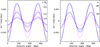 |
Fig. 1. Tidal velocity in the azimuthal direction δω″ computed with the n-layer TIDES numerical simulation (Case 30 in Table 2; continuous lines) compared to the analytical expression (Eq. (6)). The abscissa is the azimuth angle measured from the sub-binary longitude. Left: equator (θ = 90°) at three radii as indicated in the legend. Right: layer at radius 6 R⊙ at colatitudes θ = 90° and 46°. |
There are three main differences between our numerical calculation and Eq. (6). First is the degree of symmetry with respect to the line connecting the stellar centers (φ′ = 0). Equation (6) predicts equal tidal bulge amplitudes while TIDES predicts an asymmetry. We note that the tidal distortion is symmetric only if R1/a ≪ 1, where a is the orbital separation, a condition that is generally used for calculations in the “weak tides” regime. Our test binary system does not satisfy this condition. Thus, the tidal perturbation at the sub-binary longitude is stronger than at the anti-binary longitude (φ″ = 180°).
The second difference is the phase shift between the maxima of the curves shown in Fig. 1. This is a likely consequence of the large viscosity in the TIDES calculation. It is interesting to note that the effect of viscosity is mainly to introduce a phase shift while not significantly affecting the tidal amplitude, a result that has also been shown to hold for tidal flows in subsurface oceans of Solar System moons (Chen 2013). The third difference is more evident in the deeper layers, for which Eq. (6) overpredicts the amplitude. This is likely related to the assumed stellar structure, since the departures from the analytical result depend on the polytropic index used to perform the numerical simulation. However, the amplitudes predicted by Eq. (6) are seen here to differ only by factors ∼1.5−2 (excluding the external layer) which is within the range of uncertainties implied by the range in adopted tidal deformation values f* mentioned above.
Finally, it is important to note that the radiation transfer effects on the tidal velocity field are generally neglected in our numerical approach and the analytical method of Scharlemann (1981). This simplification may lead to an excessively large response of the surface layer to the tidally forced oscillations. The excess amplitude was shown by Zahn (1975) to be damped down when radiative dissipation is taken into account. This process could be incorporated in future versions of our model.
3.2. Initial uniform rotation
The general characteristic of the angular velocity of a perturbed star in a circular orbit whose core rotates with a velocity that is 1.8 times that of the orbital angular velocity is illustrated in the top panels of Fig. 2. The rotation angular velocity as measured in the star’s rest frame, ω″, is plotted as a function of azimuth angle φ′, where φ′ = 0 corresponds to the sub-binary longitude. This plot shows a similar sinusoidal morphology as that illustrated in Fig. 1, but with a significantly larger amplitude. The left panels correspond to Case 3 in Table A.1, which is computed with a polytropic index n = 1.5 and the right panels to Case 31, which is computed with n = 3 and show that the response to the tidal force is influenced by the internal stellar structure. The reason for this is that the models with larger polytropic indices are more centrally condensed, which means that the density declines more rapidly with radius. Hence, the restoring action of gas pressure is weaker than in the n = 1.5 models allowing the volume elements to attain faster velocities.
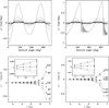 |
Fig. 2. Results for supersynchronous rotation in a circular orbit for polytropic indices n = 1.5 (left, Case 3) and n = 3 (right, Case 31). Top: angular velocity (⟨ω″⟩+δω″) at the equator in the ten layers used for this calculation. Dashes correspond to layers closest to the surface, r/R⊙ = 6.65 and 6.22. The abscissa is azimuth angle measured in degrees with φ′ = 0 corresponding to the sub-binary longitude. Bottom: meridional ω″ profiles at the equator for a selection of meridians φ′ as indicated by the labels. The abscissa is the radius at the midpoint of each layer. The behavior for r/R⊙ < 5 is shown on an amplified scale in the inset. |
The faster velocities that are evident in the surface layer of the n = 3 model cause two additional effects. The first is a significantly larger phase lag in the outer layers, compared to a smaller polytropic index model. The second is the appearance of high-frequency oscillations, most evident in the surface, which results from the faster tidal velocities, leading to nonlinearities in the system.
As it is evident that the shape of the ω″ profile changes from one meridian to the next, we use the term meridional ω″ profile to describe the dependence of ω″ over radius at a fixed azimuthal angle φ′. This is illustrated in the bottom panels of Fig. 2 where we plot a selection of the meridional ω″ profiles. This representation is useful, for example, for comparing the velocity structure of different models, as in Fig. 3 (left) which shows that the larger polytropic index allows for steeper meridional ω″ profiles. The right panel of this figure shows the manner in which the results are affected by the choice of the layer thickness. For the internal layers, the angular velocity is relatively unaffected by this parameter (Fig. 3, right). However, the velocity of the surface layer (and on occasion, the layer below it) does depend on this parameter. This is because the radius of the surface grid point (always chosen as the midpoint of the layer) is larger for a thinner layer, and is thus subjected to a larger external force than the midpoint of a thicker layer. A second (nonphysical) factor is a consequence of the computational limitations. Specifically, the time that is required for the outer layer to attain the stationary state is significantly longer than that of the inner layers. Thus, unless the objective is to model the behavior of the surface (for example, for the calculation of spectral line profile variability), it is not cost-effective to run the simulation beyond the time for which the inner layers have attained the stationary state. The dependence of ω″ on other input parameters is analyzed in the appendix.
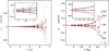 |
Fig. 3. Comparison of the meridional ω″ profiles: Left: polytropic indices n = 1.5 (Case 3) and n = 3 (dots, Case 31); Right: for layer thicknesses dR/R1 = 0.03 (black, Case 11) and 0.06 (red, Case 3). The angles that are labeled correspond to Case 11. |
Given the convenience of an analytical representation for the tidal velocity field, the natural question that arises concerns the limits of applicability of Eq. (6). This is explored in Fig. 4, which again shows the result of our Case 31 numerical simulation compared to δω″ obtained from Eq. (6), but scaled so as to compare more favorably with the numerical simulation. We find that the required scaling is less than a factor of ∼2 for all layers except the stellar surface. This suggests that Eq. (6) may be used as a rough first approximation to the tidal velocity field for circular orbits in which the average velocity structure is close to uniform.
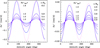 |
Fig. 4. Tidal angular velocity δω″ computed with the n-layer TIDES numerical simulation (Case 31 in Table A.1; continuous lines) compared to the scaled analytical expression (Eq. (6)). The scaling for each radius is listed in the center and the radius on the right side of each panel. The abscissa is the azimuth angle measured from the sub-binary longitude. Left: layers closest to the surface. Right: layers closest to the core. |
3.3. Initial differential rotation
An example of the results that are obtained from a model in which the computation is initiated with differential rotation is shown in Fig. 5. The initial angular velocity distribution is listed in Table 3 and is displayed in the right panel of Fig. 5 with crosses connected by a dash line. Its very steep shape was inspired by the Meynet & Maeder (2000) evolutionary models near the end of the core hydrogen burning phase, but is otherwise arbitrary. As discussed in Appendix C, the manner in which the temporal evolution proceeds leads to results that are insensitive to the precise shape of the initial ω″ profile.
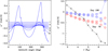 |
Fig. 5. Results for a star with an initial steep differential rotation structure (Case 34). Left: angular velocity at the equator at Day 196. Each curve corresponds to one of the layers, as labeled on the right side of the curves, where 1 corresponds to the deepest layer. Right: ω″ profiles at Day 76 (square) and Day 196 (pentagon) for azimuth angles at which the velocity gradient is greatest. The crosses connected by a dash line indicate the initial ω″ profile at the start of the computation. |
Initial differential rotation structure and structure after 196 days (Case 34).
Recalling that ω″ = ⟨ω″⟩+δω″ (Eq. (3)), we now define the term ⟨ω″⟩ profile to be the variation over radius of the average angular velocity and our results show that the ⟨ω″⟩ profile flattens over time. Thus, at any time during the computation, the tidal velocity δω″ is superposed on what may be regarded as the background differential rotation structure defined by ⟨ω″⟩. When ⟨ω″⟩→0, one may consider the star to be in a state of average uniform rotation upon which a tidal component is superposed. It is only when δω″ → 0 that one may speak of a true uniform rotation structure.
Figure 5 (right) presents the ω″ profiles for azimuth angles at which δω″ has the largest amplitude. There are two sets of curves for each of the times chosen for this illustration, 76 d and 196 d after the start of the calculation. Each set of curves shows the extrema of angular velocities and encloses the azimuthally averaged angular velocity ⟨ω″⟩ (not shown in the figure). By Day 76, the ⟨ω″⟩ profile has flattened significantly, with only a weak average differential rotation structure still present. We find that the flattening first occurs very rapidly but then systematically slows down as average uniform rotation is approached. We plot ω″ versus φ′ in the left panel of Fig. 5, showing that a differential rotation structure at Day 196 still persists but is flatter than the one at which the computation was started.
An additional feature that we observe is that the tidal amplitude δω″ of each layer depends on the degree of asynchronicity of the particular layer. This results from the dependence of δω″ on the instantaneous value of the average synchronicity parameter ⟨β(r)⟩ = ⟨ω(r)⟩/Ω0. Specifically, the tidal amplitude is larger for larger departures from synchronicity, as is also evident from Eq. (6).
We note that since it is the value of ⟨β(r)⟩ that determines the tidal amplitude of a particular layer, and not β0 (the core synchronicity parameter), this means that, from an observational perspective, an evolving value of ⟨β(R*)⟩ could lead to patterns that change on timescales longer than the orbital timescale. Here, R* represents the layers from which the dominant photospheric absorption lines arise. For example, if these layers approach a state in which ⟨β(R*)⟩ ≃ 1, the tidal flow amplitudes would diminish considerably as would any spectral variability associated with these flows.
4. The ω″ profile in eccentric orbits
In the previous section, we showed that the azimuthal tidal velocities in circular-orbit binary stars retain a general sinusoidal-like shape as a function of azimuth angle similar to that predicted by the analytical expression in Eq. (6), albeit with different amplitudes, and that this shape remains relatively stable as a function of orbital phase in the reference frame that rotates with the companion (S′). In this section, we examine the manner in which this behavior changes in an eccentric binary system. This question has already been addressed for the surface layer in the primary star of the α Virginis (Spica) system by Harrington et al. (2009) where the azimuthal dependence of the tidal velocity was found to have very pronounced, small frequency oscillations superposed on a general sinusoidal shape and was found to be orbital-phase dependent. Here, we now extend the analysis to layers below the surface.
The azimuth-dependent shape of ω″ and the ω″ profiles in the eccentric e = 0.1 Case 35 model are shown in Fig. 6. The most striking differences with respect to the analogous circular orbit case is the larger tidal amplitude, even at apastron and high-frequency oscillations, the latter similar to those reported by Harrington et al. (2009) based on the one-layer model. Additionally, the inner layers develop a differential rotation in which the gradient of the ⟨ω″⟩ profile increases over time.
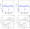 |
Fig. 6. Angular velocity and meridional ω″ profiles at the equator for the eccentric binary Case 35. The inset shows the r/R⊙ < 6 layers, which have developed an average differential rotation structure. The amplitudes and ω″ profiles change between periastron and apastron. |
Some of the differences with respect to the e = 0 analogous cases can be understood by recalling that the periastron distance is smaller than the semimajor axis of the equivalent circular orbit. Also, we recall that  describes the asynchronicity at periastron and that the instantaneous value, β(r, t) increases over orbital phase between periastron and apastron. As mentioned in Appendix C, the tidal amplitude δω″ increases with increasing β(r, t). Hence, there is an interplay between these two processes. In addition, it is important to note that the “equilibrium tide” configuration (as described, for example, by the Scharlemann 1981 equations) holds as long as the perturbations caused by the tidal force are small enough so that the fluid has time to adjust to the altered hydrostatic conditions. This is clearly not the case in the eccentric binary models, thus leading to the observed oscillations and strong departure from the equilibrium tide configuration displayed particularly by the outer layers. We note also that a similar comment applies to e = 0 models in which the product νρ is smaller than a critical threshold, as is evident in the right panel of Fig. 3.
Finally, the appearance of a positive gradient in the ⟨ω″⟩ profile of the inner layers is perplexing. It seems to counterbalance the significant negative gradient in the outer layers, which clearly is a result of the retarding effect of the tidal force, and which would be expected also for the inner layers. This curious result may simply be a consequence of the neglect of feedback into the orbital motion in the TIDES code. Specifically, if the angular momentum loss of the outer layers were to be transferred to the orbital motion, this would avoid it being transferred to the inner layers through the viscous coupling. However, the timescale over which the positive gradient develops in our calculations (≤100 d) is too fast compared to the tidal timescales (assumed to be ∼107 yr), unless the viscosity is at least ∼108 smaller, if not more. Also, if the effect were due to the neglect in TIDES of feedback to the orbital motion, one might also expect it to appear in the circular orbit calculations (that are initiated with a uniform rotation structure) but here it is not evident, as shown in Fig. 7. On the other hand, the tidal amplitude in all the layers is always larger for the positive velocities than the negative velocities. Thus, the average velocity that is computed over all azimuths is always > 0, hence feeding a positive angular momentum. This effect is more pronounced in the eccentric case than in the analogous circular because of the closer orbital separation at periastron and because of the larger β at apastron. This issue remains to be further analyzed, although we note that Hut (1981) finds regimes in which a supersynchronous binary star may increase its rotation rate instead of decreasing it, depending on the ratio of angular momenta in the orbit and the stellar rotation.
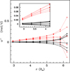 |
Fig. 7. Meridional ω″ profiles at the equator for the circular orbit Case 31 (black) and the eccentric Case 35 (red); both models have polytropic index n = 3. |
5. Discussion
5.1. Relevance for mixing: Vertical shear instability
The physical mechanisms that transport chemical elements from the nuclear-processing region toward the surface are driven by a complex interplay between temperature, velocity and chemical gradients, and their implementation into stellar structure models is generally parametrized through the use of diffusion coefficients as discussed in Zahn (1993), Heger et al. (2000), Maeder & Meynet (2000), Mathis et al. (2004, 2007), Prat & Lignières (2014), Garaud & Kulenthirarajah (2016), Garaud (2020), and references therein.
The basic idea is that shear instabilities can lead to turbulent eddies that then propagate through the fluid carrying with them the chemical abundances of the region from which they originated. The turbulent eddies propagating in the vertical direction (that is, parallel to the stellar radius), provide transport from the core to the surface. Those propagating horizontally (within a shell at a fixed radius) tend to homogenize the chemical abundances in that shell, but are also found to generate turbulence that propagates vertically.
In this section we illustrate the manner in which the TIDES code calculations can contribute toward assessing whether the shear instability may be triggered in deep layers, near the core, and thus examine the role of the tidal effects in mixing. We base this analysis on the results of numerical experiments that are reported in Garaud & Kulenthirarajah (2016), Garaud (2020), where the instability criteria are provided.
In a fluid in which the temperature and/or chemical composition is stratified, the displacement of turbulent eddies in the vertical direction is limited by the buoyancy force which tends to restore them to their equilibrium location, thus rendering the fluid stable against the shear instabilities unless Ri < Ricrit. Here, Ricrit is a critical value that is typically thought to be of order unity (Richardson 1920; Zahn 1992), and Ri is the Richardson number:
 (7)
(7)
where S = |dv/dr| is the local shearing rate of the flow field v and N is the buoyancy frequency,
 (8)
(8)
where ∇ad = (∂lnT/∂lnP)ad is the gradient at constant entropy and composition, and ∇ = dlnT/dlnP. Hp is the pressure scale height and g the gravity.
Typical stars have values Ri ≫ 1, suggesting that they are stable against this instability. This is true also for binaries. Adopting the tidal velocity δv″ as the typical flow velocity of the parcels of fluid that are interacting, one finds Ri ≥ 103 for all layers except perhaps the surface. However, if a vertically displaced parcel of fluid has time to undergo heat transfer that allows it to rapidly come into thermal equilibrium with its new surroundings, the correct criterion for shear instability is now the one associated with diffusive shear instabilities4 (Zahn 1974; Lignières 1999; Prat & Lignières 2014):
 (9)
(9)
where (RiPr)c ∼ 0.007 (Prat & Lignières 2014; Garaud & Kulenthirarajah 2016) and the Prandl number Pr = Pe/Re = ν/κT. Here, Pe is the Péclet number, Re = UL/ν is the Reynolds number, ν is the molecular kinematical viscosity, κT is the thermal diffusivity, U is a characteristic velocity scale and L the corresponding length scale.
The condition in Eq. (9) for the onset of the diffusive shear instability is valid only if heat transfer occurs rapidly, which corresponds to a low Péclet number (LPN), Pe < 1 (Lignières 1999), a condition that is met only near the stellar surface. However, because the definition of the Péclet number depends on a length scale and a velocity scale that need to be identified, Lignières (1999) associated these with the turbulent scales and defined a turbulent Péclet number,
 (10)
(10)
where urms is the rms flow velocity of turbulent eddies and ℓv is their vertical scale and suggested that criterion Eq. (9) is valid for Pet ≪ 1, even if Pe > 1. The problem then is to obtain the values of urms and ℓv. The analysis performed by Garaud & Kulenthirarajah (2016) leads to the conclusion that, for shearing motions that are caused by imposing a force F0, one can associate urms with the typical velocity that results. That is, urms = UF with,
 (11)
(11)
where F0 is the perturbing force per unit volume, ρ0 is the background density, and the length scale is renamed in terms of a unit length scale k−1. The condition for the LPN Pet ≪ 1 is now assessed using
 (12)
(12)
and if it is satisfied, the instabilities will be triggered if
 (13)
(13)
where RiF and PrF now refer to the Richardson and Prandtl numbers evaluated using UF,
We use below the convenient expressions for the Péclet, Reynolds and Richardson numbers provided by Garaud & Kulenthirarajah (2016) (their Eqs. (30) and (31)):
 (14)
(14)
The primary contribution of the TIDES models to the above considerations is that it can directly provide values of the acceleration term F0/ρ0 = dVφ″/dt, where Vφ″ = rsin(θ)δω″ is the azimuthal component of the tidal velocity. We illustrated this application of the TIDES models with the example that follows.
We performed a TIDES calculation that is tailored to a stellar structure model that provides internal structure data needed for the values of N. The chosen model has 10 M⊙ at an age of 12 Myr and an initial rotation velocity 150 km s−1 and is taken from the rotating massive main-sequence stars grids of Brott et al. (2011). The age is based on the results of Tkachenko et al. (2016). The density structure of this model is close to that of a n = 3.5 polytrope, and the radius is R1 = 5.48 R⊙. These values were used to compute Case 41 (see Table 2). Given this radius and an orbital period of 4.01 d, the synchronicity parameter of the core is  = 2.2. The resulting angular velocities at the equator are shown in Fig. 8.
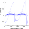 |
Fig. 8. Angular velocity ⟨ω″⟩+δω″ at the equator from a TIDES calculation for the model that is used to evaluate the shear instabilities (Case 41 in Table 2). The curves correspond to the ten layers used in these calculations, with dashes corresponding to layers closest to the surface, r/R⊙ = 5.0 and 5.3. The abscissa is azimuth angle measured in degrees with φ′ = 0 corresponding to the sub-binary longitude. |
The stellar structure radial model grid is significantly finer than in the TIDES calculation, so we averaged the stellar structure parameter values over intervals of r ± ΔR1/4, with ΔR1/4 = 0.08 R⊙. We used ν = 10 cm2 s−1 for the molecular kinematical viscosity, and for κT we visually interpolated its values from Fig. 7 of Garaud & Kulenthirarajah (2016).
Given the shape of δω″, it is clear that the acceleration term is not constant but depends on the φ′ coordinate. The φ′ dependence maps into a variation over time at a fixed position φ″ when we apply the transformation which, for circular orbits is φ′ = φ″ − (Ω0 − ω0)t. Given the sinusoidal-like shape of the variation, the acceleration term oscillates between a maximum and a minimum value passing through zero. Thus we adopt as a measure of the azimuthal acceleration,
 (15)
(15)
where rmid is the midpoint of a stellar layer and Δt is the time difference between maximum and minimum angular velocity. These maximum and minimum values obtained from Case 41 are listed in Table 4 as a function of radius and for three latitudes.
TIDES angular velocities M = 10 M⊙, R = 5.48 R⊙, Vrot = 150 km s−1, 12 Myr model.
Recalling that the general shape of the tidal velocity is similar to that given by Eq. (6) (except in the outer layers) and that this equation, when scaled, approximately matches the tidal velocity obtained with TIDES (Fig. 4), we see that the time dependence of the acceleration term goes as cos4(θ)sin(2φ″ − 4πΦ(1.−β0)), where Φ = t/P, and Φ is the orbital phase and P the orbital period. A plot of this sine function for our P = 4 d,  = 2.2 model shows that the time between a maximum and its closest minimum is ∼0.2 in orbital phase. Thus, we set Δt = 0.8 d. For the length scale we adopt a value half the size of the layers that were modeled, k−1 = ΔR/2.
The results of substituting the velocity values at the equator into Eq. (14) are listed in Table 5 (under the section labeled “Vert”), where it can be seen that the LPN condition PeF ≪ 1 is satisfied only very near the surface. Thus, even though the condition given by Eq. (13) is satisfied throughout, the diffusive shear instability in the LPN approximation does not appear to be triggered. Similar results are obtained for other latitudes.
Diffusive shear instability. M = 10 M⊙, R = 5.48 R⊙, 12 Myr model.
The high Péclet number regime is only briefly discussed in Garaud & Kulenthirarajah (2016). They report that the system transitions from intense mixing events in which the existing shear is destroyed to periods of quiescence during which the flow is nearly laminar and where the shear is gradually amplified by the forcing, until intense mixing resumes. A similar cyclical nature for the instabilities at high Péclet number has been found in laboratory experiments (Meyer & Linden 2014). Whether such behavior can occur in the deep stellar layers remains to be assessed. However, it is interesting to note that the sin(2φ′) term in the time derivative of Eq. (6) implies a time dependence. Large amounts of shear may be triggered near the maximum in the flow velocity, after building up during the prior times within each flow cycle. Thus, it seems like the occurrence of shear instabilities in the high Péclet number regime cannot be excluded at this time as a mechanism contributing toward mixing.
In addition to the above, it is important to add that the shearing motions are associated with energy dissipation. Because the amplitude of the tidal velocity increases with stellar radius, so does the energy dissipation rate. If this were to significantly decrease the temperature stratification, it would weaken the effect of the buoyancy force.
Another consideration is the potential stellar mass dependance of any mixing induced by the tidal flows for the following reasons. First, the increase in the importance of radiation pressure with increasing mass weakens the stability of the stratification. In addition, due to pronounced peaks in the radiative opacity coefficient as function of temperature, several convection zones may appear in the subsurface layers of massive main sequence stars (Cantiello et al. 2009). These convection zones, which are thought to induce observable turbulent velocity fields at the stellar surface, will also induce statistical pressure fluctuations in the layers beneath (Grassitelli et al. 2015) which may interact with the periodic tidal forcing.
In conclusion, although diffusive vertical shear instabilities in the LPN regime are excluded as a mixing process in layers close to the convective core, the same cannot yet be said about the high Péclet limit regime and particularly when the oscillating nature of the tidal flows is considered, given that such a scenario has not been fully analyzed from the fluid dynamics perspective. Furthermore, the tidal shear energy dissipation, strong radiation pressure and localized regions of sub-photospheric convection may all contribute to reduce the stratification, triggering the instability.
Finally, we note that the tidal velocity field is also present in low-mass binary stars in asynchronous rotation. However, unlike the massive main sequence stars in which altering the surface chemical abundances requires mixing from the central convective core throughout the entire radiative envelope, the lower-mass stars present boron abundance anomalies associated with layers closer to the surface. This is because boron is destroyed by proton capture, for example, in the inner ∼90% of the radiative envelope of a 15 M⊙ main sequence star (Fliegner et al. 1996), mixing would need to occur only in the outermost layers in order to produce a drop in the boron surface abundance. While rotationally induced mixing is a strong contender to produce such mixing (Proffitt et al. 2016), the tidal mixing discussed here may have an additional impact in short-period massive pre-Roche-lobe-overflow binaries.
5.2. Relevance for mixing: Horizontal shear instability
A second type of shearing flows initially discussed by Zahn (1992) are those caused by velocity differences over latitude. In this case, the horizontal shear generates secondary turbulent eddies that propagate in the vertical direction, thus potentially contributing toward mixing in this direction. The stability of these flows in the high Péclet number regime has recently been analyzed by Garaud (2020), where now the bifurcation parameter that divides the stable from the unstable regimes is:
 (16)
(16)
where
 (17)
(17)
The parameters U and L are the actual characteristic horizontal flow velocity and length scale, respectively. We now use (Garaud 2020):
where the symbol B is analogous to the Richardson number and denotes the ratio of the buoyancy frequency to the horizontal shearing rate.
As in the previous section, we used the velocities obtained in the Case 41 TIDES model and listed in Table 4 to quantify the above parameters. Specifically, we set U = rmid[sin(θ1)⟨ω″(θ1)⟩ − sin(θ2)⟨ω″(θ2)⟩] and Ly ∼ rmid(θ1 − θ2) where θ1 and θ2 correspond to two adjacent colatitudes. Choosing from Case 41 θ1 = 90° and θ2 = 72.5° and the corresponding average velocity values ⟨ω″⟩ and substituting into the above relations, we get values of ℓz and wrms, which when substituted into Eq. (16) yield Pet.
We list the results in Table 5 under the section labeled Horiz. We find that the conditions Pet ≪ 1 and BPr ≪ 0.007 are simultaneously met not only near the surface, but now also at r/R⊙ ≤ 3. Thus, this suggests that the horizontal shear instability may be triggered in stellar layers that lie relatively close to the nuclear burning core. Clearly, the same caveats mentioned in the previous section apply here and a more conclusive answer must await further developments in the fluid dynamics computations (see, for example Park et al. 2021).
5.3. Implications for binary star observations
Interactions in binary stars can be classified into two general classes. The first includes binary systems where only the observational diagnostics are affected, with no impact on the stellar structure. These interactions are: physical eclipses, which cause variations in the total measured light; wind eclipses, in which the stellar wind from one star absorbs and scatters light from the companion (see, for example, Münch 1950); Wind-wind collisions, in which the two stars possess a stellar wind that collides far from the stellar photosphere, producing excess emission at certain wavelengths and distorting the profiles of lines that are formed within the winds.
The second class includes all stars in which the presence of a companion has an impact on the internal structure and subsequent evolution. The most evident members of this class are systems undergoing Roche lobe overflow or wind accretion, and those in which the companion finds itself embedded in the extended post-main sequence envelope of the primary star and intervenes in its ejection. Less evident members are stars whose surfaces are shocked by the companion’s stellar wind, are subjected to external irradiation, or undergo tidally induced oscillations. In the first two of these processes, only the external layers are likely to be affected. Tidal perturbations, however, penetrate deeper layers and, in addition, the associated frequencies may resonante with the normal oscillation modes of the star (see Fig. 9).
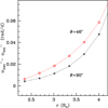 |
Fig. 9. Difference of maximum and minimum angular velocity at the equator and at colatitude 46° from the Case 41 model. Only layers at r < 4.2 R⊙ are illustrated. The abscissa is the midpoint radius of the layer. |
Tidally induced oscillations are detected through photometric and photospheric line-profile variability. The observed oscillation in the light curves are generally analyzed in the context of theoretical frameworks described in Kumar et al. (1995), Fuller (2017) and Guo et al. (2020), and references therein. The theoretical study of analogous effects in the spectral lines has been significantly more limited. Calculations from first principles of the line profile and its orbital phase-dependent variability were performed for the eccentric binaries ϵ Orionis (Moreno et al. 2005) and α Virginis (Harrington et al. 2009, 2016; Palate et al. 2013a,b) and a sample of other massive binary systems known to exhibit line-profile variability (Palate et al. 2013b). These studies used the one-layer TIDES model and confirmed that the Doppler shifts due to the horizontal component of the tidal perturbation dominate over the radial component (see Harrington et al. 2009, Fig. 13).
In the case of Spica, for which a large set of spectroscopic observations were available, the TIDES model adequately predicted the periodic changes in the photospheric absorption-line wings and the presence of discrete features that travel from the blue to the red wing of the line. A detailed fit to the line profiles and variations was not attempted because of uncertainties in the orbital inclination and stellar properties, which have become available more recently (Tkachenko et al. 2016). Also, a phase-difference between predicted and observed profiles was hypothesized to possibly be associated with the neglect of layers below the stellar surface.
Although revisiting the line-profile variability of Spica is beyond the scope of this paper, we used the n-layer version of the TIDES code to explore the extent to which the azimuthal motions of the surface layer are influenced by the layers below. In Fig. 10 the surface angular velocity from the one-layer TIDES model at periastron obtained with the same input parameters as used in Harrington et al. (2009) is compared with the n-layer TIDES model using the same input parameters (Case 25 in Table A.1). The general shape of both curves is very similar, showing broad maxima around φ′ ∼ 100° and 300° and high-frequency oscillations around φ′ ∼ 0° and 200°. However, the high-frequency oscillations are significantly different and the maxima are broader in the n-layer calculation. Both of these will have an effect on the detailed structure of the line profiles and their variability, but not the more general features that are detectable through observations. Also noteworthy is that the n-layer TIDES model predicts variations in the variability pattern over long timescales, thus allowing for the possibility of superorbital periodicities, contrary to the one-layer model which predicts strictly orbital phase-locked variations over long timescales.
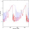 |
Fig. 10. Comparison of the azimuthal velocity predicted with the one-layer TIDES model (red) used in Harrington et al. (2009) and the n-layer model discussed in this paper (blue dash, Case 25 in Table A.1). Both curves correspond to the periastron. |
The amplitude of observed tidal effects depends on the orbital inclination because the perturbations are strongest at and around the equatorial latitude5. Curiously, some observational evidence can be found supporting the idea that tidal effects influence the results obtained from spectroscopic analyses. Mahy et al. (2020) obtained chemical abundances for a sample of massive stars, members of 32 double-line binary systems. Using their data for m sin i3 and Mspec (their Table 1), one may deduce an estimate for sin(i), the orbital inclination. In Fig. 11 we plot the derived nitrogen abundance (from their Table 2) as a function of sin(i) and find a clear trend for larger N-abundance with larger inclination angle. Whether this implies a non-homogeneous distribution of nuclear-processed elements or whether the tidal effects introduce an as yet unaccounted for bias in the data analysis remains to be ascertained. If most binary stars do not develop strong shear instabilities, the latter would be most likely. However, further analysis is needed to shed light on this issue.
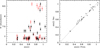 |
Fig. 11. Data from Mahy et al. (2020) suggesting a possible correlation between nitrogen abundance and orbital inclination (left). Black squares correspond to the primary component and red triangles to the secondary of each system. Right: orbital inclination deduced from the data in Mahy et al. (see text) for the primary and secondary components of the binary systems. |
An additional implication of the results that we present in this paper is the dependence on the synchronicity parameter β of the tidal velocity amplitude: The further β departs from synchronicity, the larger the oscillation amplitude. Here, β is the ratio between the stellar rotation angular velocity and the instantaneous orbital angular velocity, and in a differentially rotating star, there are different values of β at different radii. Furthermore, in eccentric binaries, the orbital angular velocity is smallest at apastron and largest at periastron. Thus, although the orbital separation at apastron is larger than at periastron, the larger value of β may induce greater surface variability than at periastron, especially for cases in which β ≃ 1 around the periastron phase. If one of the processes driving mass loss is associated with stellar pulsations (see, for example, Townsend 2007; Kraus et al. 2015), then phenomena that depend on the mass loss rate (such as wind-wind collision emission and accretion onto a companion) may not present themselves as expected from models that only take the orbital separation into account.
Finally, we address the apparently curious result obtained by Pavlovski et al. (2018) whose analysis of a sample of massive binary stars failed to reveal the expected correlation between stellar rotation velocity and surface chemical composition. In light of the numerical simulations presented here in Sect. 2.6, this result might not be unexpected. As already pointed out by Koenigsberger & Moreno (2013), binaries that are tidally locked in the strict sense of the term, meaning that β = 1 at all times and in all layers, have very stable structures and rapidly damp out differential rotation and localized flows that would have otherwise contributed to the mixing efficiency. Additional observational evidence supporting the idea that differential rotation may be suppressed in tidally locked low-mass stars has been presented by Hussain et al. (2006) and discussed by Collier Cameron (2007). A more controversial question concerns the effect on meridional circulation currents. The recent analysis by Hastings et al. (2020) leads to the conclusion that the mixing efficiency due to meridional currents in tidally locked binaries should be significantly larger than in their single-star counterparts. The results of Pavlovski et al. (2018) indicate the contrary, thus leading to the speculation that meridional currents may be if not suppressed, at least diminished, in tidally locked systems.
6. Summary of results and conclusions
Binary stars are generally assumed to be tidally locked and thus their internal mixing processes are assumed to follow those of single stars in uniform rotation (but see Hastings et al. 2020). However, the picture changes for eccentric-orbit binaries, for young stars that have not had time to circularize and synchronize their orbits, and for stars that are undergoing core contraction and envelope expansion as they evolve off the main sequence. These systems are all in asynchronous rotation, a condition in which tidal flows introduce a 3D time-varying rotation structure. Scharlemann (1981) provided an analytical expression that quantifies the amplitude of these flows when the departure from equilibrium is very small. In this paper we illustrate a method for arbitrary rotation rates and eccentricity.
Our method is based on an upgraded version of the TIDES code, which solves the equations of motion on a 3D grid of volume elements. The equations of motion include gravitational, centrifugal, Coriolis, gas pressure and viscous forces and they are solved simultaneously with the orbital motion of the companion. The model does not include the effects of buoyancy and meridional circulation, nor does it include thermal diffusivity or radiative transport, all of which have an impact on the evolution over time of the rotation structure (Goldreich & Schubert 1967; Garaud & Kulenthirarajah 2016). However, as our model is used only to compute the behavior of angular velocity over short timescales (less than a few decades), neglecting the effects with long timescales is not likely to significantly impact our results.
In circular-orbit binaries with moderate departures from synchronicity, the angular velocity at a fixed position on the perturbed star, ω″, undergoes sinusoidal-like oscillations that are driven by the tidal forcing. The amplitude and frequency of the oscillations grow with growing departures from synchronicity. For these systems, the analytical expression of Scharlemann (1981) is shown to reproduce the azimuthal component of the tidal velocity within factors of ∼2, even though this expression was derived for much smaller departures (∼1%) from synchronicity and convective envelopes. This suggests the potential use of the analytical expression to obtain a rough estimate of the tidal amplitudes. In the cases of large departures from synchronicity and in eccentric-orbit binaries, ω″ is distorted from the sinusoidal-like shape and it undergoes localized high-frequency oscillations. Characterizing these high-frequency oscillations requires numerical simulations such as those that we present in this paper. Such oscillations may now be observed through high precision photometry of objects such as the “heartbeat” stars (see, for example, Fuller 2017; Guo et al. 2020),
The instantaneous value of ω″ as a function of radius, latitude, and longitude that is provided by our calculations can be used to inform on the potential impact of the tidal interactions on the mixing processes. As an example, we examined whether the velocity amplitudes in the internal layers of our test binary are able to trigger the diffusive shear instability in the context of the constraints that are given in Garaud & Kulenthirarajah (2016) and Garaud (2020), and we find that the conditions for triggering the horizontal diffusive shear instability may be met in layers that lie relatively close to the stellar core. We note, however, that the constraints were not derived for a time-dependent oscillating fluid such as the tidal flows, and thus further work is needed to address this issue.
We analyzed the angular velocity averaged over the azimuth angle at a fixed latitude and its dependence on radius, which we call the ⟨ω″⟩ profile. We showed that an initially pronounced differential rotation structure flattens over time and tends toward uniform rotation on the viscous timescale. For the viscosity values considered in this paper (3−160 × 1013 cm2 s−1), the ⟨ω″⟩ profile → constant on τ < 250 yr, which is negligible compared to most evolutionary timescales.
We discussed some of the observational implications that may be drawn from our numerical experiments. For example, the instantaneous value of β in eccentric binaries depends on the orbital phase, reaching maximum at apastron. Thus, physical processes that may be affected by the tidally induced perturbations (such as high-frequency oscillations and mass loss) may be orbital-phase-dependent if their characteristic timescales are short enough. Thus, we propose that the synchronicity parameter β and its orbital-phase dependence be taken into account when analyzing eccentric systems. For tidally locked systems we find that perturbations are rapidly damped down, providing a possible explanation for the observational finding that the mixing efficiency in some of these systems appears to be lower than expected given their rotation rate (Pavlovski et al. 2018).
We uncover a curious result in observational data that suggests higher derived nitrogen abundances in binaries with larger orbital inclinations. If real, this would suggest an inhomogeneous chemical distribution over the stellar surface, although a more likely explanation may reside in the tidal perturbations, which are strongest at the equator, and may distort the spectral lines that are used for the abundance determinations.
In our analysis we have neglected the effects of radiative damping, feedback between rotation and orbital motion and magnetic fields. The latter may be omnipresent in the stellar interior (see for example, Takahashi & Langer 2021). It has been suggested that internal magnetic fields reduce the radial shear in stars (Eggenberger et al. 2005; Heger et al. 2005; Suijs et al. 2008), which is also required by observations (Deheuvels et al. 2014; Mosser et al. 2012). On the other hand, the growth time of the tidally induced oscillations is very short, and the associated shear motion reverses periodically, such that it may be possible that the shearing rates obtained by our models persist even when magnetic fields are considered. Future investigations are needed to address these issues.
The TIDES code is available upon request and is easily implemented in any operating system running a Fortran or GNU Fortran compiler. The particular versions used to produce the results in this paper are named lx.osc.disip.2.2.f (one layer), lx.capas.vr0.3.1.f (n layers).
It is also dependent on time but on significantly longer timescales than those considered in this paper.
We can write  = rsin(θ)(ω′−⟨ω′⟩). For a circular orbit, ω′ = ω″ + ω0 − Ω0. Using this relation (which also applies to
  ) and the definition in Eq. (3), Vφ = rsin(θ)(ω″ − ⟨ω″⟩) = rsin(θ)δω″, since
  = 0 by definition.
Also known as “secular shear instability”.
We offer a reminder that in our model the stellar and orbital angular velocity vectors are parallel. Other configurations may lead to different implications.
Acknowledgments
We thank an anonymous referee for comments and suggestions that significantly improved this paper. GK is grateful to Frédéric Masset and Fabian R. N. Schneider who commented and made helpful suggestions on an earlier draft of this paper, and to Matteo Cantiello, Francois Leyvraz, Luis Mochan and Sergio Cuevas for many helpful discussions. We acknowledge support from Conacyt project 252499 and UNAM/PAPIIT IN103619.
References
- Aerts, C., Mathis, S., & Rogers, T. M. 2019, ARA&A, 57, 35 [NASA ADS] [CrossRef] [MathSciNet] [Google Scholar]
- Alexander, M. E. 1973, Ap&SS, 23, 459 [NASA ADS] [CrossRef] [Google Scholar]
- Brott, I., de Mink, S. E., Cantiello, M., et al. 2011, A&A, 530, A115 [NASA ADS] [CrossRef] [EDP Sciences] [Google Scholar]
- Cantiello, M., Langer, N., Brott, I., et al. 2009, A&A, 499, 279 [NASA ADS] [CrossRef] [EDP Sciences] [Google Scholar]
- Chen, E. M. 2013, PhD Thesis, University of California, Santa Cruz, USA [Google Scholar]
- Collier Cameron, A. 2007, Astron. Nachr., 328, 1030 [NASA ADS] [CrossRef] [Google Scholar]
- De Marco, O., & Izzard, R. G. 2017, PASA, 34, e001 [Google Scholar]
- de Mink, S. E., Cantiello, M., Langer, N., et al. 2009, A&A, 497, 243 [NASA ADS] [CrossRef] [EDP Sciences] [Google Scholar]
- Deheuvels, S., Doğan, G., Goupil, M. J., et al. 2014, A&A, 564, A27 [NASA ADS] [CrossRef] [EDP Sciences] [Google Scholar]
- Dolginov, A. Z., & Smel’Chakova, E. V. 1992, A&A, 257, 783 [Google Scholar]
- Eggenberger, P., Maeder, A., & Meynet, G. 2005, A&A, 440, L9 [NASA ADS] [CrossRef] [EDP Sciences] [Google Scholar]
- Ekström, S., Georgy, C., Eggenberger, P., et al. 2012, A&A, 537, A146 [NASA ADS] [CrossRef] [EDP Sciences] [Google Scholar]
- Fliegner, J., Langer, N., & Venn, K. A. 1996, A&A, 308, L13 [NASA ADS] [Google Scholar]
- Fuller, J. 2017, MNRAS, 472, 1538 [NASA ADS] [CrossRef] [Google Scholar]
- Gagnier, D., Rieutord, M., Charbonnel, C., Putigny, B., & Espinosa Lara, F. 2019, A&A, 625, A89 [NASA ADS] [CrossRef] [EDP Sciences] [Google Scholar]
- Garaud, P. 2020, ApJ, 901, 146 [Google Scholar]
- Garaud, P., & Kulenthirarajah, L. 2016, ApJ, 821, 49 [Google Scholar]
- Goldreich, P., & Schubert, G. 1967, ApJ, 150, 571 [Google Scholar]
- Grassitelli, L., Fossati, L., Simón-Diáz, S., et al. 2015, ApJ, 808, L31 [NASA ADS] [CrossRef] [Google Scholar]
- Guo, Z., Shporer, A., Hambleton, K., & Isaacson, H. 2020, ApJ, 888, 95 [CrossRef] [Google Scholar]
- Harrington, D., Koenigsberger, G., Moreno, E., & Kuhn, J. 2009, ApJ, 704, 813 [NASA ADS] [CrossRef] [Google Scholar]
- Harrington, D., Koenigsberger, G., Olguín, E., et al. 2016, A&A, 590, A54 [NASA ADS] [CrossRef] [EDP Sciences] [Google Scholar]
- Hastings, B., Langer, N., & Koenigsberger, G. 2020, A&A, 641, A86 [EDP Sciences] [Google Scholar]
- Heger, A., Langer, N., & Woosley, S. E. 2000, ApJ, 528, 368 [NASA ADS] [CrossRef] [Google Scholar]
- Heger, A., Woosley, S. E., & Spruit, H. C. 2005, ApJ, 626, 350 [NASA ADS] [CrossRef] [Google Scholar]
- Hussain, G. A. J., Allende Prieto, C., Saar, S. H., & Still, M. 2006, MNRAS, 367, 1699 [NASA ADS] [CrossRef] [Google Scholar]
- Hut, P. 1981, A&A, 99, 126 [NASA ADS] [Google Scholar]
- Koenigsberger, G., & Moreno, E. 2013, in EAS Publications Series, eds. K. Pavlovski, A. Tkachenko, & G. Torres, 64, 339 [NASA ADS] [CrossRef] [EDP Sciences] [Google Scholar]
- Koenigsberger, G., & Moreno, E. 2016, Rev. Mex. Astron. Astrofis., 52, 113 [NASA ADS] [Google Scholar]
- Koenigsberger, G., Moreno, E., & Harrington, D. M. 2012, A&A, 539, A84 [NASA ADS] [CrossRef] [EDP Sciences] [Google Scholar]
- Kraus, M., Haucke, M., Cidale, L. S., et al. 2015, A&A, 581, A75 [NASA ADS] [CrossRef] [EDP Sciences] [Google Scholar]
- Kumar, P., Ao, C. O., & Quataert, E. J. 1995, ApJ, 449, 294 [NASA ADS] [CrossRef] [Google Scholar]
- Langer, N. 1991, A&A, 243, 155 [Google Scholar]
- Langer, N. 1998, A&A, 329, 551 [NASA ADS] [Google Scholar]
- Langer, N. 2012, ARA&A, 50, 107 [NASA ADS] [CrossRef] [Google Scholar]
- Langer, N., Heger, A., & Fliegner, J. 1997, in IAU Symp., eds. T. R. Bedding, A. J. Booth, & J. Davis, 189, 343 [NASA ADS] [Google Scholar]
- Lanza, A. F., & Mathis, S. 2016, Celest. Mech. Dyn. Astron., 126, 249 [NASA ADS] [CrossRef] [Google Scholar]
- Lignières, F. 1999, A&A, 348, 933 [NASA ADS] [Google Scholar]
- Lovekin, C. C. 2020, Front. Astron. Space Sci., 6, 77 [CrossRef] [Google Scholar]
- Maeder, A. 1987, A&A, 178, 159 [NASA ADS] [Google Scholar]
- Maeder, A., & Meynet, G. 2000, ARA&A, 38, 143 [Google Scholar]
- Mahy, L., Sana, H., Abdul-Masih, M., et al. 2020, A&A, 634, A118 [NASA ADS] [CrossRef] [EDP Sciences] [Google Scholar]
- Mathis, S., Palacios, A., & Zahn, J. P. 2004, A&A, 425, 243 [NASA ADS] [CrossRef] [EDP Sciences] [Google Scholar]
- Mathis, S., Palacios, A., & Zahn, J. P. 2007, A&A, 462, 1063 [NASA ADS] [CrossRef] [EDP Sciences] [Google Scholar]
- Mathis, S., Prat, V., Amard, L., et al. 2018, A&A, 620, A22 [NASA ADS] [CrossRef] [EDP Sciences] [Google Scholar]
- Meyer, C. R., & Linden, P. F. 2014, J. Fluid Mech., 753, 242 [NASA ADS] [CrossRef] [Google Scholar]
- Meynet, G., & Maeder, A. 2000, A&A, 361, 101 [NASA ADS] [Google Scholar]
- Moreno, E., & Koenigsberger, G. 1999, Rev. Mex. Astron. Astrofis., 35, 157 [NASA ADS] [Google Scholar]
- Moreno, E., Koenigsberger, G., & Toledano, O. 2005, A&A, 437, 641 [NASA ADS] [CrossRef] [EDP Sciences] [Google Scholar]
- Moreno, E., Koenigsberger, G., & Harrington, D. M. 2011, A&A, 528, A48 [NASA ADS] [CrossRef] [EDP Sciences] [Google Scholar]
- Mosser, B., Goupil, M. J., Belkacem, K., et al. 2012, A&A, 540, A143 [NASA ADS] [CrossRef] [EDP Sciences] [Google Scholar]
- Münch, G. 1950, ApJ, 112, 266 [NASA ADS] [CrossRef] [Google Scholar]
- Ogilvie, G. I. 2014, ARA&A, 52, 171 [Google Scholar]
- Pablo, H., Richardson, N. D., Fuller, J., et al. 2017, MNRAS, 467, 2494 [NASA ADS] [CrossRef] [Google Scholar]
- Palate, M., Koenigsberger, G., Rauw, G., Harrington, D., & Moreno, E. 2013a, A&A, 556, A49 [NASA ADS] [CrossRef] [EDP Sciences] [Google Scholar]
- Palate, M., Rauw, G., Koenigsberger, G., & Moreno, E. 2013b, A&A, 552, A39 [NASA ADS] [CrossRef] [EDP Sciences] [Google Scholar]
- Park, J., Prat, V., Mathis, S., & Bugnet, L. 2021, A&A, 646, A64 [EDP Sciences] [Google Scholar]
- Pavlovski, K., Southworth, J., & Tamajo, E. 2018, MNRAS, 481, 3129 [NASA ADS] [Google Scholar]
- Penev, K., Sasselov, D., Robinson, F., & Demarque, P. 2007, ApJ, 655, 1166 [Google Scholar]
- Penev, K., Barranco, J., & Sasselov, D. 2009, ApJ, 705, 285 [NASA ADS] [CrossRef] [Google Scholar]
- Prat, V., & Lignières, F. 2014, A&A, 566, A110 [NASA ADS] [CrossRef] [EDP Sciences] [Google Scholar]
- Press, W. H., Smarr, L. L., & Wiita, P. J. 1975, ApJ, 202, L135 [NASA ADS] [CrossRef] [Google Scholar]
- Proffitt, C. R., Lennon, D. J., Langer, N., & Brott, I. 2016, ApJ, 824, 3 [NASA ADS] [CrossRef] [Google Scholar]
- Richard, D., & Zahn, J.-P. 1999, A&A, 347, 734 [Google Scholar]
- Richardson, L. F. 1920, Proc. R. Soc. London Ser. A, 97, 354 [NASA ADS] [CrossRef] [Google Scholar]
- Scharlemann, E. T. 1981, ApJ, 246, 292 [NASA ADS] [CrossRef] [Google Scholar]
- Song, H. F., Maeder, A., Meynet, G., et al. 2013, A&A, 556, A100 [NASA ADS] [CrossRef] [EDP Sciences] [Google Scholar]
- Suijs, M. P. L., Langer, N., Poelarends, A. J., et al. 2008, A&A, 481, L87 [NASA ADS] [CrossRef] [EDP Sciences] [Google Scholar]
- Takahashi, K., & Langer, N. 2021, A&A, 646, A19 [NASA ADS] [CrossRef] [EDP Sciences] [Google Scholar]
- Talon, S., Zahn, J. P., Maeder, A., & Meynet, G. 1997, A&A, 322, 209 [NASA ADS] [Google Scholar]
- Tassoul, J.-L. 1987, ApJ, 322, 856 [NASA ADS] [CrossRef] [Google Scholar]
- Tassoul, J. L., & Tassoul, M. 1982, ApJ, 261, 265 [CrossRef] [Google Scholar]
- Tkachenko, A., Matthews, J. M., Aerts, C., et al. 2016, MNRAS, 458, 1964 [NASA ADS] [CrossRef] [Google Scholar]
- Toledano, O., Koenigsberger, G., & Moreno, E. 2007a, in Massive Stars in Interactive Binaries, eds. N. St.-Louis, & A. F. J. Moffat, ASP Conf. Ser., 367, 437 [NASA ADS] [Google Scholar]
- Toledano, O., Moreno, E., Koenigsberger, G., Detmers, R., & Langer, N. 2007b, A&A, 461, 1057 [NASA ADS] [CrossRef] [EDP Sciences] [Google Scholar]
- Townsend, R. 2007, in Unsolved Problems in Stellar Physics: A Conference in Honor of Douglas Gough, eds. R. J. Stancliffe, G. Houdek, R. G. Martin, & C. A. Tout, AIP Conf. Ser., 948, 345 [NASA ADS] [CrossRef] [Google Scholar]
- Vidal, J., Cébron, D., ud-Doula, A., & Alecian, E. 2019, A&A, 629, A142 [CrossRef] [EDP Sciences] [Google Scholar]
- Welsh, W. F., Orosz, J. A., Aerts, C., et al. 2011, ApJS, 197, 4 [Google Scholar]
- Zahn, J. P. 1974, in Stellar Instability and Evolution, eds. P. Ledoux, A. Noels, & A. W. Rodgers, 59, 185 [NASA ADS] [CrossRef] [Google Scholar]
- Zahn, J. P. 1975, A&A, 41, 329 [NASA ADS] [Google Scholar]
- Zahn, J. P. 1992, A&A, 265, 115 [NASA ADS] [Google Scholar]
- Zahn, J. P. 1993, Space Sci. Rev., 66, 285 [NASA ADS] [CrossRef] [Google Scholar]
- Zahn, J. P. 2008, in EAS Pub. Ser., eds. M. J. Goupil, & J. P. Zahn, 29, 67 [Google Scholar]
Appendix A: Method and examples
All models and case numbers.
Initial uniform rotation velocities.
Initial non-uniform rotation velocities (a) and (c).
The full set of models that were computed for this paper is listed in Table A.1. Column 1 lists the case number, Col. 2 indicates the value of the core asynchronicity parameter  , Col. 3 the viscosity value (in units of
  d−1), Col. 4 the layer thickness, and Col. 5 the number of layers. Column 6 indicates the initial rotation condition, where uniform rotation is described by the constant
  value while nonuniform rotation is described by (a), (b), (c), (f) and the values listed in the footnote to this table. Column 7 lists the number of orbital cycles over which the run was performed. The last column of the table indicates other input parameters that were varied from their nominal values, specifically, eccentricity e, the number of azimuthal or latitudinal elements Nφ, Nθ and the secondary mass m2. The number following these variable names gives the modified value.
The rotation angular velocities in the inertial reference frame S and the rotating frame S′ are listed for the initial uniform rotation cases in Table A.2. The equatorial rotation velocity at the surface of the equivalent rigidly rotating stars is 0 km s−1 ( = 0), 86 km s−1 (
 = 1) and 155 km s−1 (
 = 1.8). The analogous list of angular velocities for the nonuniform initial rotation states (a) and (c) are listed in Table A.3.
A.1. Transitory, stationary and equilibrium states
An example of the temporal evolution of  is illustrated in Fig. A.1 for cases with
  = 0 (nonrotating, Case 17), 1.8 (super-synchronous, Case 1), and 1 (synchronous, Case 15). The synchronous case converges to uniform rotation while the asynchronous cases converge to one in which
  is stratified, with maximum amplitude at the surface.
Examples of synchronous rotation are illustrated in Figs. A.1 and A.2. These are Cases 15 and 16 in Table A.1, and are presented here to illustrate the stability of the TIDES numerical algorithm. Even when the initial conditions depart significantly from the equilibrium state, the calculation converges to the equilibrium state. In Case 15, the star is unperturbed and is in uniform synchronous rotation at the start of the calculation. When the perturbation due to the companion’s gravitational field is applied, the star undergoes large amplitude oscillations as it adjusts to the presence of the external potential. As is shown in the main plot of Fig. A.1, the perturbed surface attains velocities as high as ∼0.25 rad d−1 which, however, rapidly decay and converge to < 5 × 10⁻¹¹ rad d−1 (corresponding to a linear velocity of ∼10−4 cm s−1) after 800 d. The layers below the surface suffer a similar but smaller amplitude initial perturbation and attain the stationary state more rapidly.
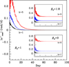 |
Fig. A.1. Evolution over time of the maximum angular velocity (absolute value) along the equator in the rest frame of the rotating primary star (S″ coordinate system) at radius 6.6 R⊙ (k = 5, red), 6.2 R⊙ (k = 4, blue) and 5.0 R⊙ (k = 1, black), where k indicates the number assigned to the layer. Initial rotation is uniform. Time zero is the start of the calculation, and the time axis in the three plots is the same. Data are smoothed using a 100-point moving average. Main plot: Synchronous rotation, Case 15 in Table A.1. Inset top: super-synchronous rotation Case 1. Inset bottom: No rotation, Case 17. |
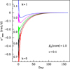 |
Fig. A.2. Evolution over time of the maximum angular velocity |


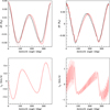 |
Fig. A.3. Results of calculations with the one-layer TIDES model using input parameters corresponding to those listed in Table A.1. Top: Surface deformation at the equator for the analogous Case 1 model (left, β0 = 1.8) and the analogous Case 17 model (right, β0 = 0). Black and red curves indicate different times within the same orbital cycle. Bottom: Radial component of the tidal velocity for each of the models shown in the top panels. |
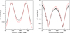 |
Fig. A.4. Angular velocity at the equator obtained with the one-layer (red) and n-layer (black) models illustrating the differences due to the neglect in the n-layer model of the radial deformation and radial velocity component. Left: Case 1 (β0 = 1.8). Right: Case 17 (β0 = 0). |
In Case 16, the calculation starts with three layers rotating slower than synchronous rotation and the layer closest to the core rotating faster. These initial velocities are tabulated in Cols. 6–8 of Table A.3. As illustrated in Fig. A.2, during the transitory state all layers converge toward ω″ = 0, as expected for the equilibrium state. In this figure, we chose to plot  instead of its absolute value as in Fig. A.1 in order to more clearly illustrate the sub-synchronous and super-synchronous motions in the perturbed star’s rest frame and the manner in which they reach the stationary state.
Number of volume elements per colatitude for Nθ = 20.
A.2. Comparison with the one-layer model
The n-layer TIDES calculation suppresses motions in the radial and polar directions. This implies that there is no tidal deformation. In this section we examine the implications of neglecting radial motion and deformation by comparing with results of the original one-layer calculation (Moreno et al. 2011). The input parameters are as in the nominal case (Case 1, Table A.1). The maximum tidal deformation is illustrated in Fig. A.3 for orbital phases distributed equally over the orbital cycle. Contrary to a static calculation, the location and amplitude of the tidal bulges undergo time-dependent variations as a consequence of the dynamical processes.
Figure A.4 compares the angular velocity in the surface layer of the Case 1 model with that obtained from the one-layer model. The most important differences are seen at azimuth angles corresponding to the tidal bulges (see Fig. A.3, which indicates the location of the tidal bulges). The explanation lies in the fact that the bulges are at a larger radius and are therefore more strongly affected by the tidal force. The difference at the sub-binary longitude is ∼0.08 rad d−1, and somewhat smaller in the opposite hemisphere. Hence, neglecting the radial deformation leads to angular velocities that are underestimated at the location of the bulges. Another difference is that the shape and amplitude of ω″ obtained with the n-layer calculation are constant with orbital phase, contrary to what is obtained from the one-layer model.
Appendix B: Dependence on input parameters
We tested the dependence of the ω″ profile on a variety of input parameter combinations, specifically Nr, ΔR/R1, ν, and polytropic index. We illustrate the ω″ profiles with the most pronounced velocity gradients in Fig. B.1 (left) for runs performed with different combinations of the first three of the above mentioned input parameters. The ω″ profiles are the same in all cases. However, models run with smaller viscosity values require a longer time to attain the same state as models that were run with greater viscosities. This also holds true for the azimuthal dependence of ω″, as illustrated in Fig. B.1 (right). This figure also shows that the same result is obtained regardless of whether the calculation is initiated in uniform rotation or with a pronounced differential rotation structure.
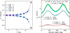 |
Fig. B.1. Sample results from tests that were performed to assess the dependence on the layer thickness ΔR/R1, number of layers Nr, and viscosity ν. Left: ω″ profiles for azimuth angles at which the most pronounced velocity gradients occur, computed with the combinations of ΔR/R1, Nr, and ν as indicated by the legend which, from top to bottom, refers to cases to Cases 1, 2, 14, 11 and 3 in Table A.1. The abscissa is the radial distance from the center of the star to the layer midpoint. Right: Surface angular velocity from models holding all input parameters constant except for ν, showing that calculations with smaller values of ν reach the same rotation state as those with larger values, but after longer times. The three curves show: Top: Case 1 at Day 397 (green), Case 6 at Day 798 (black), Case 7 at Day 2004 (cyan). Middle: Case 7 at Day 798 (cyan), Case 8 at Day 8024 (red). Bottom: Case 6 at Day 36 (black), Case 8 at Day 2003 (red). |
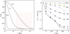 |
Fig. B.2. Tests performed for different polytropic indices n, where γ = 1+1/n, the exponent of the polytropic equation of state. Left: Polytropic density structures as a function of radius for the 6.84 R⊙ models. Density is given in units of ρc, the central density. Each curve is labeled with its corresponding value of n. The vertical lines indicate the base of layers for layer thickness ΔR/R1 = 0.06. Right: Azimuthally averaged angular velocity ⟨ω″⟩ for n = 1.5 (square, Case 1), 3.0 (triangle, Case 32b) and 4.5 (large cross, Case 51). Illustrated are the values for times t/day = 4, 36, 76, and 197 after the start of the calculation, showing that all cases converge toward average uniform rotation. The initial ω″ profile is shown with the asterisks joined by a continuous line. |
Results of tests with different polytropic indices (n = 1.5, 3 and 4.5) are illustrated in Fig. B.2 (right). The corresponding density structures are shown in Fig. B.2 (left). The most significant difference in the results occurs for n = 4.5 because uniform average rotation is approached much more slowly than the other cases, particularly in the outer layers. This is explained by the fact that such a large polytropic index corresponds to a star with a more pronounced density gradient and thus the transport of angular momentum in these layers is less efficient than in the case of smaller values of n.
Case 4 ( = 1.8) and Case 21 (
 = 2.1) were used to explore the effect of different degrees of synchronicity. In both cases, the average rotation tends toward uniform, but with a faster final rotation speed in Case 21 as expected. Also, the tidal amplitude is larger for Case 21 than Case 4, as can be verified by comparing the data in Tables B.1 and B.2. Tests with
  = 1.1, 1.4, and 1.9 confirm that the tidal amplitude increases with increasing departures from synchronicity. It is important to note, however, that in order to attain average uniform rotation in a super-synchronously rotating star, the outer layers may approach the critical speed at which surface material can become detached. The equatorial latitude would be the first to experience this instability, thus potentially leading to equatorial outflows.
Azimuthally averaged angular velocity and tidal amplitude Case 4:  = 1.8, ν = 0.1
  d−1.
d−1.
Azimuthally-averaged angular velocity and tidal amplitude Case 21:  = 2.1, ν = 0.1
  d−1.
d−1.
Case 17 is one of various tests performed for a nonrotating (β0 = 0) star and which serves to illustrate the case of sub-synchronous rotation. The surface angular velocity is shown in Fig. A.4. It is noteworthy that although the core is nonrotating, the tidal flows at the surface on the equator attain speeds of ∼0.4 rad d−1, which from an observational standpoint is relevant for the interpretation of the line broadening in observed spectra. That is, depending on the orientation of the orbital axis with respect to an observer, the detected spectroscopic line profiles could simulate a v sin i as large as 20 km s−1 (i being the inclination of the orbital plane with respect to the observer), despite the fact that the star is nonrotating.
Appendix C: Temporal evolution of the ⟨ω″⟩ profile
We find that, excluding angular momentum redistribution processes other than the viscous interaction between layers, an initially steep differential rotation structure tends to flatten over time, first rapidly, and then progressively slower as the star approaches the average uniform rotation state. We take a closer look at this process using the results of Cases 6, 7 and 8 from Table A.1. These models have a smaller radial grid size than some of the others discussed in this paper because the layers that lie closest to the surface are the slowest to approach uniform rotation so they determine the timescale over which the average uniform rotation state is attained. Hence, it is computationally more efficient to focus on these layers. The initial differential rotation considered here is the same as that of the 5 outer layers of the larger radial grid models (see Table 3).
The procedure followed is to calculate the values of ⟨ω″⟩ at several times after the start of the calculation and for calculations performed for several viscosity values. The result is illustrated in Fig. C.1 (left). The three viscosity values yield the same result: the ⟨ω″⟩ profile flattens over time but the timescale increases with decreasing viscosity value. In addition, we find that the same ⟨ω″⟩ profile is obtained regardless of the viscosity value, given enough time for the flattening to occur. For example, it takes 2003 d for the ⟨ω″⟩ profile in the model computed with ν = 5 × 10⁻⁴  d−1 to equal the profile at Day 36 in the model with ν1 = 0.028
  d−1.
d−1.
Not only does the ⟨ω″⟩ profile behave in this manner but also the ω″ dependence on azimuth angle (as shown in Fig. B.1), at least within the range of viscosities that we used in our simulations. This result is useful for, among other things, allowing us to employ a relatively large viscosity value so as to accelerate the approach to the stationary state in the computations. Now, defining a viscous timescale τvis = r2/ν and using r = 6.63 R⊙, the surface radius, Fig. C.1 (right) confirms that the time that it takes for the surface to (almost) corotate with the core is τvis, for the range of viscosities that we used.
The fact that ⟨ω″⟩≃0 is approached asymptotically on the viscous timescale τvis = r2/ν brings to light the importance of constraining the viscosity value, since for turbulent viscosity 1010 < ν < 1014 cm2 s−1 (Penev et al. 2007), the surface of our Case 6 binary star attains average uniform rotation on timescales ranging from one yr to 600 thousand years. Although this timescale corresponds to only a small fraction of the ∼12 Myr lifetime of a star like Spica’s primary, viscosities on the low end of the range would require consideration of wind mass loss, meridional currents and orbital evolution, which are here neglected. However, for the larger values of ν in the above range, the timescale for reaching average uniform rotation is significantly shorter than that of these other processes, which suggests that stars with very large ν values may effectively be considered to be in average uniform rotation.
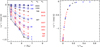 |
Fig. C.1. Evolution from differential rotation to average uniform rotation for three different viscosity values, ν1/( |


All Tables
TIDES angular velocities M = 10 M⊙, R = 5.48 R⊙, Vrot = 150 km s−1, 12 Myr model.
Azimuthally averaged angular velocity and tidal amplitude Case 4: = 1.8, ν = 0.1 d−1.
Azimuthally-averaged angular velocity and tidal amplitude Case 21: = 2.1, ν = 0.1 d−1.
All Figures
|
Fig. 1. Tidal velocity in the azimuthal direction δω″ computed with the n-layer TIDES numerical simulation (Case 30 in Table 2; continuous lines) compared to the analytical expression (Eq. (6)). The abscissa is the azimuth angle measured from the sub-binary longitude. Left: equator (θ = 90°) at three radii as indicated in the legend. Right: layer at radius 6 R⊙ at colatitudes θ = 90° and 46°. |
| In the text | |
|
Fig. 2. Results for supersynchronous rotation in a circular orbit for polytropic indices n = 1.5 (left, Case 3) and n = 3 (right, Case 31). Top: angular velocity (⟨ω″⟩+δω″) at the equator in the ten layers used for this calculation. Dashes correspond to layers closest to the surface, r/R⊙ = 6.65 and 6.22. The abscissa is azimuth angle measured in degrees with φ′ = 0 corresponding to the sub-binary longitude. Bottom: meridional ω″ profiles at the equator for a selection of meridians φ′ as indicated by the labels. The abscissa is the radius at the midpoint of each layer. The behavior for r/R⊙ < 5 is shown on an amplified scale in the inset. |
| In the text | |
|
Fig. 3. Comparison of the meridional ω″ profiles: Left: polytropic indices n = 1.5 (Case 3) and n = 3 (dots, Case 31); Right: for layer thicknesses dR/R1 = 0.03 (black, Case 11) and 0.06 (red, Case 3). The angles that are labeled correspond to Case 11. |
| In the text | |
|
Fig. 4. Tidal angular velocity δω″ computed with the n-layer TIDES numerical simulation (Case 31 in Table A.1; continuous lines) compared to the scaled analytical expression (Eq. (6)). The scaling for each radius is listed in the center and the radius on the right side of each panel. The abscissa is the azimuth angle measured from the sub-binary longitude. Left: layers closest to the surface. Right: layers closest to the core. |
| In the text | |
|
Fig. 5. Results for a star with an initial steep differential rotation structure (Case 34). Left: angular velocity at the equator at Day 196. Each curve corresponds to one of the layers, as labeled on the right side of the curves, where 1 corresponds to the deepest layer. Right: ω″ profiles at Day 76 (square) and Day 196 (pentagon) for azimuth angles at which the velocity gradient is greatest. The crosses connected by a dash line indicate the initial ω″ profile at the start of the computation. |
| In the text | |
|
Fig. 6. Angular velocity and meridional ω″ profiles at the equator for the eccentric binary Case 35. The inset shows the r/R⊙ < 6 layers, which have developed an average differential rotation structure. The amplitudes and ω″ profiles change between periastron and apastron. |
| In the text | |
|
Fig. 7. Meridional ω″ profiles at the equator for the circular orbit Case 31 (black) and the eccentric Case 35 (red); both models have polytropic index n = 3. |
| In the text | |
|
Fig. 8. Angular velocity ⟨ω″⟩+δω″ at the equator from a TIDES calculation for the model that is used to evaluate the shear instabilities (Case 41 in Table 2). The curves correspond to the ten layers used in these calculations, with dashes corresponding to layers closest to the surface, r/R⊙ = 5.0 and 5.3. The abscissa is azimuth angle measured in degrees with φ′ = 0 corresponding to the sub-binary longitude. |
| In the text | |
|
Fig. 9. Difference of maximum and minimum angular velocity at the equator and at colatitude 46° from the Case 41 model. Only layers at r < 4.2 R⊙ are illustrated. The abscissa is the midpoint radius of the layer. |
| In the text | |
|
Fig. 10. Comparison of the azimuthal velocity predicted with the one-layer TIDES model (red) used in Harrington et al. (2009) and the n-layer model discussed in this paper (blue dash, Case 25 in Table A.1). Both curves correspond to the periastron. |
| In the text | |
|
Fig. 11. Data from Mahy et al. (2020) suggesting a possible correlation between nitrogen abundance and orbital inclination (left). Black squares correspond to the primary component and red triangles to the secondary of each system. Right: orbital inclination deduced from the data in Mahy et al. (see text) for the primary and secondary components of the binary systems. |
| In the text | |
|
Fig. A.1. Evolution over time of the maximum angular velocity (absolute value) along the equator in the rest frame of the rotating primary star (S″ coordinate system) at radius 6.6 R⊙ (k = 5, red), 6.2 R⊙ (k = 4, blue) and 5.0 R⊙ (k = 1, black), where k indicates the number assigned to the layer. Initial rotation is uniform. Time zero is the start of the calculation, and the time axis in the three plots is the same. Data are smoothed using a 100-point moving average. Main plot: Synchronous rotation, Case 15 in Table A.1. Inset top: super-synchronous rotation Case 1. Inset bottom: No rotation, Case 17. |
| In the text | |
|
Fig. A.2. Evolution over time of the maximum angular velocity |
| In the text | |
|
Fig. A.3. Results of calculations with the one-layer TIDES model using input parameters corresponding to those listed in Table A.1. Top: Surface deformation at the equator for the analogous Case 1 model (left, β0 = 1.8) and the analogous Case 17 model (right, β0 = 0). Black and red curves indicate different times within the same orbital cycle. Bottom: Radial component of the tidal velocity for each of the models shown in the top panels. |
| In the text | |
|
Fig. A.4. Angular velocity at the equator obtained with the one-layer (red) and n-layer (black) models illustrating the differences due to the neglect in the n-layer model of the radial deformation and radial velocity component. Left: Case 1 (β0 = 1.8). Right: Case 17 (β0 = 0). |
| In the text | |
|
Fig. B.1. Sample results from tests that were performed to assess the dependence on the layer thickness ΔR/R1, number of layers Nr, and viscosity ν. Left: ω″ profiles for azimuth angles at which the most pronounced velocity gradients occur, computed with the combinations of ΔR/R1, Nr, and ν as indicated by the legend which, from top to bottom, refers to cases to Cases 1, 2, 14, 11 and 3 in Table A.1. The abscissa is the radial distance from the center of the star to the layer midpoint. Right: Surface angular velocity from models holding all input parameters constant except for ν, showing that calculations with smaller values of ν reach the same rotation state as those with larger values, but after longer times. The three curves show: Top: Case 1 at Day 397 (green), Case 6 at Day 798 (black), Case 7 at Day 2004 (cyan). Middle: Case 7 at Day 798 (cyan), Case 8 at Day 8024 (red). Bottom: Case 6 at Day 36 (black), Case 8 at Day 2003 (red). |
| In the text | |
|
Fig. B.2. Tests performed for different polytropic indices n, where γ = 1+1/n, the exponent of the polytropic equation of state. Left: Polytropic density structures as a function of radius for the 6.84 R⊙ models. Density is given in units of ρc, the central density. Each curve is labeled with its corresponding value of n. The vertical lines indicate the base of layers for layer thickness ΔR/R1 = 0.06. Right: Azimuthally averaged angular velocity ⟨ω″⟩ for n = 1.5 (square, Case 1), 3.0 (triangle, Case 32b) and 4.5 (large cross, Case 51). Illustrated are the values for times t/day = 4, 36, 76, and 197 after the start of the calculation, showing that all cases converge toward average uniform rotation. The initial ω″ profile is shown with the asterisks joined by a continuous line. |
| In the text | |
|
Fig. C.1. Evolution from differential rotation to average uniform rotation for three different viscosity values, ν1/( |
| In the text | |
Current usage metrics show cumulative count of Article Views (full-text article views including HTML views, PDF and ePub downloads, according to the available data) and Abstracts Views on Vision4Press platform.
Data correspond to usage on the plateform after 2015. The current usage metrics is available 48-96 hours after online publication and is updated daily on week days.
Initial download of the metrics may take a while.