© K. Mandal et al. 2021

1. Introduction

Rossby waves are named after their discoverer, Carl-Gustaf Rossby, who first explained the largest scale oscillatory motions on Earth’s atmosphere (Rossby 1939) to arise from the conservation of potential vorticity. Chelton & Schlax (1996) observed these oscillations in the ocean by analyzing variations in the sea-surface height from satellite data. These large-scale motions have implications on terrestrial weather and can influence convection and differential rotation in stars if they have sufficient amplitudes (Plaskett 1966). Rossby-like waves, also known as r-modes in the astrophysical context, can be sustained by any rotating spherical fluid body, such as the Sun, in which the Coriolis force acts as a restoring force (Papaloizou & Pringle 1978; Provost et al. 1981; Saio 1982). These waves have frequencies comparable to the rotation rate. For a uniformly rotating star, Rossby modes follow the dispersion relation (Provost et al. 1981)

$$\begin{array}{c}\hfill \sigma =-\frac{2\mathrm{\Omega }t}{s(s+1)},\end{array}$$(1)

in a corotating frame, where s and t are the harmonic degree and azimuthal order of these modes, respectively¹. The availability of long-term high-resolution observational data of the Sun from Mount Wilson Observatory, the Michelson Doppler Imager (MDI) on-board the Solar and Heliospheric Observatory (SOHO), and Global Oscillation Network Group (GONG) have inspired several authors (e.g., Kuhn et al. 2000; Ulrich 2001; Sturrock et al. 2015) to search for these oscillatory motions in the Sun. Sturrock et al. (2015) observed oscillations in solar radius measurements and attributed them to be due to r modes with t = 1. All these earlier studies lacked the measurement of the dispersion relation of these modes, which is critical to characterizing and understanding them. Löptien et al. (2018) were the first to measure the dispersion relation of these waves in the Sun using surface-granulation tracking methods and ring-diagram analysis with 6 years of SDO/Helioseismic and Magnetic Imager (HMI) data and unambiguously detected modes with azimuthal order starting from t = 3 to t = 15. The surface eigenfunctions are close to sectoral spherical harmonics, although they are more peaked about the equator as a result of the effect of differential rotation (Gizon et al. 2020). The detection of Rossby modes was later confirmed by several authors using different methods, for example, by Liang et al. (2019) who used time-distance helioseismology, by Hanson et al. (2020) and Proxauf et al. (2020) who used ring-diagram analysis, and by Hanasoge & Mandal (2019) who applied normal-mode coupling (for a description of the method, see Woodard 1989; Lavely & Ritzwoller 1992; Roth & Stix 2003; Woodard et al. 2013). Interested readers are referred to Zaqarashvili et al. (2021) and references therein for a detailed review on Rossby waves in the Sun and other astrophysical problems.

Although very powerful in its scope and inferential quality, the method of mode coupling is only slowly gaining traction in helioseismology (see Schad & Roth 2020; Hanson et al. 2021; Kashyap et al. 2021, for some other recent developments with this method); for instance, there is limited work on characterizing its limitations and developing mitigation strategies. The detection of Rossby modes by Hanasoge & Mandal (2019) using this method added an important milestone to this methodology. Mandal & Hanasoge (2020) compared properties of these modes, for example, the frequency and line width, with the prior work by Löptien et al. (2018) and Liang et al. (2019), and they developed an approach to mitigate systematic errors that arise in this method, such as leakage in the spatial domain because of our limited vantage of the Sun. Hanasoge & Mandal (2019) and Mandal & Hanasoge (2020) considered coupling between acoustic modes with the same harmonic degrees. They detected Rossby modes only in the sectoral power spectra. Their measurement was not sensitive to even harmonic degrees which limited their detection to Rossby modes with odd harmonic degrees only. Here, we consider couplings between acoustic modes with different harmonic degrees and report the first detection of sectoral Rossby modes with even harmonic degrees using this method.

2. Data analysis

Line-of-sight Doppler velocity, Φ, observed by space-based observatories, including SOHO/MDI (Scherrer et al. 1995) and SDO/HMI (Schou et al. 2012), and ground-based observatories, including GONG, are the main inputs to helioseismology. The data are transformed into the spherical-harmonic domain to obtain Φ_ℓm, where (ℓ,m) are the harmonic degree and azimuthal order of the p mode. As described earlier, we use s and t to indicate the harmonic degree and azimuthal order of the Rossby waves to avoid confusion. A detailed discussion about how this data product is obtained from line-of-sight Doppler velocity data may be found in Larson & Schou (2015). We obtain these time series from the JSOC website². We perform a temporal Fourier transform on the data to obtain ${\mathrm{\Phi }}_{\mathcal{l}m}^{\omega }$, where ω is the temporal frequency. The next step is to perform cross correlations across wave numbers, that is, ${\mathrm{\Phi }}_{\ell m}^{\omega \ast }{\mathrm{\Phi }}_{\ell +\mathrm{\Delta }\ell m+t}^{\omega +\sigma }$, where σ is varied to capture the time dependence of the perturbation and the difference between the two azimuthal order, t, captures the length scale of the perturbation. We note that Δℓ is the difference between harmonic degrees of the two acoustic modes of interest. For the problem of Rossby waves, we know the dispersion relation analytically for a uniformly rotating fluid body with an angular rotation rate Ω, which in the corotating frame (at the same rotational frequency) is given by Eq. (1).

The observed latitudinal eigenfunctions of these modes, labeled by only azimuthal order t, which may have contributions from sectoral (s = |t|) and nonsectoral modes (s ≠ |t|) (Löptien et al. 2018; Proxauf et al. 2020) peak at the equator and switch sign near  30° latitude at the surface. Latitudinal eigenfunctions of these modes cannot have any zero-crossings if these modes are purely sectoral. This can either be explained by considering the presence of nonsectoral modes (Proxauf et al. 2020) or due to the effect of differential rotation on the Rossby mode eigenfunction (Gizon et al. 2020). In this work, we do not attempt to answer the abovementioned aspect of Rossby modes. Though normal mode coupling can easily distinguish between sectoral and non-sectoral Rossby modes, we only focus on sectoral ones in this work. In that case, the dispersion relation (Eq. (1)) simplifies to

$$\begin{array}{c}\hfill \sigma =-\frac{2\mathrm{\Omega }}{(s+1)}·\end{array}$$(2)

We choose Ω/2π = 453.1 nHz, corresponding to the equatorial rotation rate of the Sun. We analyze the first 4 years of SDO/HMI data, from 2010 to 2014. We also analyze 8 years of SDO/HMI data from 2010 to 2018. The reason for choosing two different data sets is to demonstrate robustness of the method, that is, it can capture signals from a shorter time series. Though we have access to a few decades of high-resolution data for the Sun, we cannot say the same in the context of asteroseismology. Therefore, if a method works with a shorter time series of data, it can also be easily extended to asteroseismology. We analyze all the p-modes in the harmonic degree range ℓ ∈ [50, 180] and for all identified radial orders, n. We slightly modify our measurements for this particular work from that of Hanasoge & Mandal (2019) and Mandal & Hanasoge (2020) as they considered correlations between acoustic modes with the same harmonic degree which are only sensitive to the odd harmonic degree of Rossby waves (see Eqs. (6) and (7) of Hanasoge 2018). For notational convenience, we use the same convention as in Hanasoge (2018) unless otherwise mentioned. Analyzing these correlation measurements at all temporal frequencies, ω, σ, and for all pairs of acoustic modes with quantum numbers (n, ℓ, m), is very cumbersome. To simplify the analysis, we measure the B-coefficient, $B_{st}^{\sigma }$ (Woodard 2016), which captures a signal due to the Rossby mode with a harmonic degree, s and azimuthal order, t from couplings between acoustic modes with identical radial orders, and Δℓ = 1, 3, which is defined as

$$\begin{array}{c}\hfill B_{st}^{\sigma }(n,\ell ,\ell +\mathrm{\Delta }\ell )=\frac{{\sum }_{m,\omega }{\gamma }_{tm}^{\ell +\mathrm{\Delta }\ell s\ell }{H}_{\ell \ell +\mathrm{\Delta }\ell mt}^{\sigma \ast }(\omega ){\mathrm{\Phi }}_{\ell m}^{\omega \ast }{\mathrm{\Phi }}_{\ell +\mathrm{\Delta }\ell m+t}^{\omega +\sigma +t\mathrm{\Omega }}}{{\sum }_{m,\omega }{|{\gamma }_{tm}^{\ell +\mathrm{\Delta }\ell s\ell }{H}_{\ell \ell +\mathrm{\Delta }\ell mt}^{\sigma \ast }|}^2},\end{array}$$(3)

where

$$\begin{array}{c}\hfill {\gamma }_{tm}^{\ell +\mathrm{\Delta }\ell s\ell }={(-1)}^{m+t}\sqrt{(2s+1)}\left(\begin{array}{ccc}\ell +\mathrm{\Delta }\ell & s& \ell \\ -(m+t)& t& m\end{array}\right),\end{array}$$(4)

and

$$\begin{array}{cc}\hfill H_{\ell \ell +\mathrm{\Delta }\ell mt}^{\sigma }(\omega )& =-2\omega L_{\ell m}^{\ell m}{L}_{\ell +\mathrm{\Delta }\ell m+t}^{\ell +\mathrm{\Delta }\ell m+t}\hfill \\ \hfill & (N_{\ell +\mathrm{\Delta }\ell }{R}_{\ell m}^{\omega \ast }|R_{\ell +\mathrm{\Delta }\ell m+t}^{\omega +\sigma +t\mathrm{\Omega }}{|}^2+N_{\ell }{|R_{\ell m}^{\omega }|}^2{R}_{\ell +\mathrm{\Delta }\ell m+t}^{\omega +\sigma +t\mathrm{\Omega }})\hfill \end{array}$$(5)

where N_ℓ is the mode normalization constant, $L_{\mathcal{l}m}^{{\mathcal{l}}^{\prime }{m}^{\prime }}$ denotes leakage from mode (n, ℓ, m) to another mode (n, ℓ′,m′) due to our limited vantage of the Sun (Schou & Brown 1994), and the expression of $R_{\mathcal{l}m}^{\omega }$ is (see Eq. (11) of Hanasoge et al. 2017)

$$\begin{array}{c}\hfill R_{\ell m}^{\omega }=\frac{1}{{({\omega }_{n\ell m}-i{\mathrm{\Gamma }}_{n\ell }/2)}^2-{\omega }^2},\end{array}$$(6)

where ω_nℓm and Γ_nℓ are the eigenfrequency and full width at half maximum of the mode, (n, ℓ, m). We analyze p-modes in the frequency range [1000, 4600] μHz. In order to capture the temporal evolution of Rossby modes, we vary σ/2π ∈ [ − 350, 0.0] nHz, sufficient to capture the temporal evolution of all Rossby modes because its maximum frequency is σ/2π = −302 nHz for (s, t) = (2, 2) (we consider only even harmonic degrees in this work). For a consistent analysis, we need to estimate noise in the measurement properly. We follow the analysis of Hanasoge (2018) to estimate the systematic noise in these measurements and use Eq. (3) to estimate the variance. Taking a sum over all frequency bins ω in Eq. (3) for all pairs of acoustic modes considered in the mode-coupling measurement is computationally very expensive. Therefore we restrict the sum to coupling between (n, ℓ, m) and (n,  ℓ+Δℓ, m + t) modes in the frequency intervals

$$\begin{array}{cc}& |\omega -{\omega }_{n\ell m}|\le {\mathrm{\Gamma }}_{n\ell }\hfill \end{array}$$(7)

$$\begin{array}{cc}\hfill & \text{and}|\omega -{\omega }_{n\ell +\mathrm{\Delta }\ell m+t}+(\sigma +t\mathrm{\Omega })|\le {\mathrm{\Gamma }}_{n\ell +\mathrm{\Delta }\ell }.\hfill \end{array}$$(8)

The reason to subtract σ + tΩ in Eq. (8) is to restrict the frequency interval to a full width around the resonance associated with (n,  ℓ+Δℓ, m + t). We then connect these measured B-coefficients with the perturbation in the medium, which in turn may be used for inference by performing an inversion as discussed in the next section.

2.1. Inversion

Rossby waves are described as a toroidal flow and may be expressed as

$$\begin{array}{c}\hfill u^{\sigma }(r,\theta ,\varphi )={\displaystyle \sum _{s,t}{w}_{st}^{\sigma }(r)\widehat{\mathbf{r}}\times {\mathbf{\nabla }}_1{Y}_{st}(\theta ,\varphi ).}\end{array}$$(9)

The Y_s t is the spherical harmonic degree with degree s and azimuthal order t and ${\mathbf{\nabla }}_1=\widehat{\theta }{\partial }_{\theta }+\frac{\widehat{\varphi }}{sin\theta }{\partial }_{\varphi }$, where $\widehat{\theta }$ and $\widehat{\varphi }$ are the unit vectors along increasing co-latitude, θ, and longitude, ϕ, direction. The term $w_{st}^{\sigma }(r)$ captures the depth dependence of the mode. We only focus on sectoral Rossby modes in this work, as discussed in Sect. 2, and consider the azimuthal order, t = s. The successful measurement of Rossby modes requires this function to attain significant amplitudes beyond the background power in the vicinity of the theoretical dispersion relation, that is, Eq. (2). If we were to use the flow profile from Eq. (9) as a perturbation to the background model, the mode eigenfunction computed using the background model would be coupled, which, after some algebra, may be estimated as (see for Hanasoge 2018)

$$\begin{array}{c}\hfill B_{\mathit{st}}^{\sigma }(n,\ell ,{\ell }^{\prime })=f_{{\ell }^{\prime }-\ell }{\displaystyle {\int }_{\odot }dr{\mathcal{K}}_{n\ell }(r)w_{\mathit{st}}^{\sigma }(r),}\end{array}$$(10)

where f_{ℓ′−ℓ,s}𝒦_nℓ corresponds to the sensitivity kernel for the coupling between mode (n, ℓ, m) and (n, ℓ′,m + t). The f_{ℓ′−ℓ,s} is obtained from the asymptotic expression of the kernel (Vorontsov 2011) as the following

$$\begin{array}{c}\hfill f_{{\ell }^{\prime }-\ell }={(-1)}^{(s+{\ell }^{\prime }-\ell -1)/2}\times \frac{(s-{\ell }^{\prime }+\ell )!!(s+{\ell }^{\prime }-\ell )!!}{\sqrt{(s-{\ell }^{\prime }+\ell )!(s+{\ell }^{\prime }-\ell )!}}\end{array}$$(11)

for odd s + ℓ′−ℓ. This form of the kernel is valid when s ≪ ℓ or s ≪ ℓ′. The usefulness of choosing the asymptotic over the exact form is due to convenience as it separates out the dependencies on s (Rossby wave degree), ℓ′−ℓ (difference between harmonic degrees of the acoustic modes of interest), and the radius into a product of a function f_{ℓ′−ℓ,s} and the kernel 𝒦_nℓ(r). We demonstrate the validity of this assumption in Fig. 1 (also see Hanasoge et al. 2017). We choose two different cases, ℓ′−ℓ = 1 and ℓ′−ℓ = 3, and compare kernels obtained using the asymptotic expression with the corresponding exact forms. It can be seen that the choice of these asymptotic kernels is valid for our problem as the maximum harmonic degree of Rossby modes s (< 20) that we are considering is less than the minimum harmonic degree of the acoustic modes (ℓ = 50) used here.

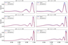Fig. 1. Comparison between exact kernels (Eq. (53) of Hanasoge 2018) in solid navy blue lines and asymptotic kernels (𝒦nℓ(r) multiplied by fℓ′−ℓ,s) in red-dashed lines for s = 6. The panels on the left and right sides are for ℓ′−ℓ = 1 and 3, respectively. We consider three different harmonic degrees ℓ = 50, 100, 150 which cover almost the entire range of harmonic degrees that we have used for data preparation. We have normalized both kernels in each panel by the maximum values of the kernel obtained from the exact expression. Both kernels match better at larger values of ℓ, as expected.

In our previous work (Hanasoge & Mandal 2019; Mandal & Hanasoge 2020), we were unable to infer even-degree Rossby modes as we only considered coupling between same-degree p-modes (see condition in Eq. (11)). Couplings between p modes with Δℓ = ℓ′ − ℓ = 1 and 3 enable us to detect Rossby waves of even harmonic degrees. In order to estimate $w_{st}^{\sigma }$ from the measured B-coefficients, $B_{st}^{\sigma }$, we need to perform inversions. We use the regularized least squares (RLS) method discussed in Mandal & Hanasoge (2020) to invert Eq. (10).

3. Results

The Rossby signal in the measured B-coefficients may be calculated by performing a weighted sum over the signed B-coefficients ${(-1)}^{\mathcal{l}}{B}_{st}^{\sigma }(n,\mathcal{l},\mathcal{l}+\mathrm{\Delta }\mathcal{l})$, over all harmonic degrees, ℓ. We then take the sum of the squares of their absolute values over all radial orders, n, to estimate the quantity $\sum _n{|\sum _{\ell }{(-1)}^{\ell }{B}_{\mathit{st}}^{\sigma }(n,\ell ,\ell +\mathrm{\Delta }\ell )/{\mathcal{N}}_{\mathit{st}}^{\sigma }(n,\ell ,\ell +\mathrm{\Delta }\ell )|}^2$, where ${\mathcal{N}}_{\mathit{st}}^{\sigma }(n,\ell ,\ell +\mathrm{\Delta }\ell )$ corresponds to measurement noise. If the measured B-coefficients capture the signal properly, we would expect to see significant power close to the theoretical dispersion relation (Eq. (2)), which is indeed the case, as seen in Fig. 2. We show results for Δℓ = 1 and Δℓ = 3 separately. The sectoral mode s = 2 does not appear when considering Δℓ = 3 since finite couplings are only possible when s ≥ Δℓ. Therefore, it can only be captured from measurements with Δℓ = 1.

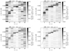Fig. 2. Estimated values of the weighted sum $\sum _n{|\sum _{\ell }{(-1)}^{\ell }{B}_{\mathit{st}}^{\sigma }(n,\ell ,\ell +\mathrm{\Delta }\ell )/{\mathcal{N}}_{\mathit{st}}^{\sigma }(n,\ell ,\ell +\mathrm{\Delta }\ell )|}^2$, using the observed B-coefficients obtained after considering the coupling between acoustic modes with Δℓ = 1 (left panel) and 3 (right) is plotted here. Upper and lower panels: results from analyses of 4 and 8 years of SDO/HMI data, respectively. The power for each azimuthal order, t, has been normalized. The black-dashed line is the theoretical dispersion relation for a uniformly rotating fluid with rotation frequency Ω/2π = 453 nHz. Modes with even azimuthal orders ranging from t = 2 to 16 are shown here.

We obtain $w_{st}^{\sigma }$ (Eq. (9)) after performing inversions described in Sect. 2 and plot $|w_{\mathit{st}}^{\sigma }{|}^2$ at the depth r = 0.98 R_⊙ in Fig. 3. The spectra show significant power close to the theoretical dispersion relation, similar to Fig. 2, for all even azimuthal orders t = 4 to 16. We do not detect power in the t = 2 sectoral mode, as seen in Fig. 5. Power close to the theoretical frequency of this mode does not stand out from the background. Prior works by Löptien et al. (2018), Liang et al. (2019), Proxauf et al. (2020), and Hanson et al. (2020) have also reached a similar conclusion. In order to place constraints on the amplitude of this mode, we highlight the anticipated t = 2 Rossby-mode frequency in Fig. 5, where no peaks rise beyond the background. Based on the strength of the background power, the nondetection of this mode implies an upper amplitude limit of 0.2 m s⁻¹. We also see significant power for the sectoral mode t = 16, though it is slightly shifted from the theoretical frequency. Indeed, we do not expect all the modes to follow the analytical dispersion relation exactly (Eq. (2)) since it is derived for the case of a uniformly rotating sphere, whereas the Sun shows radial and latitudinal differential rotation. Other factors, for example, convection and the magnetic field, are not accounted for in Eq. (2). The detection of the s = 16 mode, were it to be independently confirmed, would highlight the resolving power of this technique since previous studies have not observed it.

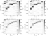Fig. 3. Normalized power $|w_{\mathit{st}}^{\sigma }{|}^2$ of sectoral Rossby modes with azimuthal orders t = 2 to 16 obtained from inverting B-coefficients at a depth of 0.98 R⊙. The black-dashed line is the theoretical dispersion relation of Rossby modes (cf. Eq. (2)) for a uniformly rotating medium at a rate of Ω/2π = 453 nHz. Upper and lower panels: results from analyses of 4 and 8 years of SDO/HMI data, respectively, also mentioned in the titles of each panel. Left and right panels: results for Δℓ = 1 and Δℓ = 3 case, respectively.

After obtaining the profile of $w_{st}^{\sigma }$ from inversions, we fit a Lorentzian function with a constant background,

$$\begin{array}{c}\hfill F(\sigma )=\frac{A}{1+{[(\sigma -{\sigma }_0)/(\mathrm{\Gamma }/2)]}^2}+D,\end{array}$$(12)

to $|w_{st}^{\sigma }{|}^2$ of these sectoral modes for each harmonic degree, s. Here A, σ₀, and Γ are the amplitude, frequency, and line-width of the mode, respectively. We note that D is the constant background power. We use power spectra obtained from 8 years of HMI data and the Δℓ = 3 case for fitting. We follow the approach of Anderson et al. (1990) and minimize the following function

$$\begin{array}{c}\hfill {\displaystyle \sum _{\sigma }lnF(\sigma )+\frac{|w_{st}^{\sigma }{|}^2}{F(\sigma )},}\end{array}$$(13)

with respect to the model parameters, A, σ₀, Γ, and D. We apply the fmin subroutine, which uses the downhill simplex algorithm, implemented in the scipy.optimize function to minimize Eq. (13). The values of these mode parameters obtained from the fitting are tabulated in Table 1. Fit spectra are shown in Fig. 4. We compare the mode frequencies from our work with prior results of Löptien et al. (2018) and Liang et al. (2019) in Table 1. We find that the Rossby-mode power peaks around t = 8, which is consistent with the previous studies by Löptien et al. (2018) and Liang et al. (2019).

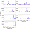Fig. 4. Analyses from 8 years of SDO/HMI data. Power spectra of even-degree sectoral Rossby modes (value mentioned in each panel) at a depth of 0.98 R⊙ are shown by solid blue lines with circles. The Lorentzian function with a constant background, as described in Sect. 3, has been fitted to these spectra to obtain the mode frequency, line-width, and amplitude. These fits are tabulated in Table 1. The fit spectrum is shown by the solid red line.

4. Discussion and conclusions

Global-mode coupling, although a well-known method, is still relatively unexplored in its applications to helioseismology. Given the challenges in understanding the data and given that it is a relatively novel measurement process, our prior work focused on same-degree couplings, which have the additional benefit of mitigating the leakage of background power into the resonances. However, this limited us to being able to only draw inferences of odd-harmonic-degree toroidal flows. We expand the set of inferences here by considering the coupling between p modes with finite harmonic-degree separation, Δℓ = 1, 3. This allows us to detect sectoral Rossby modes with even azimuthal numbers in the Sun over the range t = 4 to 16. Similar to earlier findings (Löptien et al. 2018; Liang et al. 2019; Proxauf et al. 2020; Hanson et al. 2020), we also do not find evidence for the sectoral mode, t = 2. There is no current understanding why the t = 2 mode is undetectable. It is evident that power in this particular mode is very small or simply does not exist (see Fig. 5), which is of interest in the context of understanding Rossby-mode excitation and dissipation. We also see evidence of sectoral-mode power beyond azimuthal number t = 15. Though we consider two cases Δℓ = 1 and 3 in this work, other cases, for example Δℓ> 3, may also be considered for this study, keeping in mind one caveat: modes with harmonic degree s < Δℓ will not be captured due to the selection rule discussed in Sect. 2. We find that the signal-to-noise ratio is better for Δℓ = 3 than Δℓ = 1 (see Fig. 3). We will investigate how the signal-to-noise ratio varies for different Δℓ in future work and whether it can be improved by combining all the seismic data together in the analysis instead of separately, as done here.

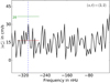Fig. 5. Power spectrum for Rossby mode (s, t) = (2, 2) from analyses of 8 years of SDO/HMI data. The blue-dashed vertical line indicates the theoretically anticipated frequency of the s = 2 sectoral mode. The solid red line indicates the background power over the frequency range [ − 342, −262] nHz. The green line corresponds to the power of the sectoral Rossby mode s = 2 with an amplitude of 20 cm s−1.

We present our results only for near-surface layers in this work. However, because we analyze couplings between global modes, we are able to infer $w_{st}^{\sigma }$ as a function of the radius after inversion. The inference of the radial dependence of these modes at both odd and even azimuthal numbers is deferred to future work; this may shed light on the excitation mechanism of these modes. Although Mandal & Hanasoge (2020) have shown that spatial leakage does not affect inferences of the radial dependencies of these modes, care must still be taken as the observed data might contain other systematic errors, which may influence the inferences. This work, taken together with our previous work (Hanasoge & Mandal 2019), highlights mode-coupling as very useful in determining the length and time scales of multiscale dynamics in the Sun.

Acknowledgments

We thank the referee for useful comments which helped to improve the manuscript. K.M. and L.G. acknowledge support from ERC Synergy grant WHOLESUN 810218. S.M.H. acknowledges the Max Planck Partner Group program.

References

All Tables

All Figures

Fig. 1. Comparison between exact kernels (Eq. (53) of Hanasoge 2018) in solid navy blue lines and asymptotic kernels (𝒦nℓ(r) multiplied by fℓ′−ℓ,s) in red-dashed lines for s = 6. The panels on the left and right sides are for ℓ′−ℓ = 1 and 3, respectively. We consider three different harmonic degrees ℓ = 50, 100, 150 which cover almost the entire range of harmonic degrees that we have used for data preparation. We have normalized both kernels in each panel by the maximum values of the kernel obtained from the exact expression. Both kernels match better at larger values of ℓ, as expected.

In the text

Fig. 2. Estimated values of the weighted sum $\sum _n{|\sum _{\ell }{(-1)}^{\ell }{B}_{\mathit{st}}^{\sigma }(n,\ell ,\ell +\mathrm{\Delta }\ell )/{\mathcal{N}}_{\mathit{st}}^{\sigma }(n,\ell ,\ell +\mathrm{\Delta }\ell )|}^2$, using the observed B-coefficients obtained after considering the coupling between acoustic modes with Δℓ = 1 (left panel) and 3 (right) is plotted here. Upper and lower panels: results from analyses of 4 and 8 years of SDO/HMI data, respectively. The power for each azimuthal order, t, has been normalized. The black-dashed line is the theoretical dispersion relation for a uniformly rotating fluid with rotation frequency Ω/2π = 453 nHz. Modes with even azimuthal orders ranging from t = 2 to 16 are shown here.

In the text

Fig. 3. Normalized power $|w_{\mathit{st}}^{\sigma }{|}^2$ of sectoral Rossby modes with azimuthal orders t = 2 to 16 obtained from inverting B-coefficients at a depth of 0.98 R⊙. The black-dashed line is the theoretical dispersion relation of Rossby modes (cf. Eq. (2)) for a uniformly rotating medium at a rate of Ω/2π = 453 nHz. Upper and lower panels: results from analyses of 4 and 8 years of SDO/HMI data, respectively, also mentioned in the titles of each panel. Left and right panels: results for Δℓ = 1 and Δℓ = 3 case, respectively.

In the text

Fig. 4. Analyses from 8 years of SDO/HMI data. Power spectra of even-degree sectoral Rossby modes (value mentioned in each panel) at a depth of 0.98 R⊙ are shown by solid blue lines with circles. The Lorentzian function with a constant background, as described in Sect. 3, has been fitted to these spectra to obtain the mode frequency, line-width, and amplitude. These fits are tabulated in Table 1. The fit spectrum is shown by the solid red line.

In the text

Fig. 5. Power spectrum for Rossby mode (s, t) = (2, 2) from analyses of 8 years of SDO/HMI data. The blue-dashed vertical line indicates the theoretically anticipated frequency of the s = 2 sectoral mode. The solid red line indicates the background power over the frequency range [ − 342, −262] nHz. The green line corresponds to the power of the sectoral Rossby mode s = 2 with an amplitude of 20 cm s−1.

In the text

References

- Anderson, E. R., Duvall, T. L., Jr., & Jefferies, S. M. 1990, ApJ, 364, 699 [NASA ADS] [CrossRef] [Google Scholar]
- Chelton, D. B., & Schlax, M. G. 1996, Science, 272, 234 [NASA ADS] [CrossRef] [Google Scholar]
- Gizon, L., Fournier, D., & Albekioni, M. 2020, A&A, 642, A178 [CrossRef] [EDP Sciences] [Google Scholar]
- Hanasoge, S. 2018, ApJ, 861, 46 [CrossRef] [Google Scholar]
- Hanasoge, S., & Mandal, K. 2019, ApJ, 871, L32 [Google Scholar]
- Hanasoge, S. M., Woodard, M., Antia, H. M., Gizon, L., & Sreenivasan, K. R. 2017, MNRAS, 470, 1404 [NASA ADS] [CrossRef] [Google Scholar]
- Hanson, C. S., Gizon, L., & Liang, Z.-C. 2020, A&A, 635, A109 [EDP Sciences] [Google Scholar]
- Hanson, C. S., Hanasoge, S., & Sreenivasan, K. R. 2021, ApJ, 910, 156 [NASA ADS] [CrossRef] [Google Scholar]
- Kashyap, S. G., Das, S. B., Hanasoge, S. M., Woodard, M. F., & Tromp, J. 2021, ApJS, 253, 47 [CrossRef] [Google Scholar]
- Kuhn, J. R., Armstrong, J. D., Bush, R. I., & Scherrer, P. 2000, Nature, 405, 544 [NASA ADS] [CrossRef] [Google Scholar]
- Larson, T. P., & Schou, J. 2015, Sol. Phys., 290, 3221 [NASA ADS] [CrossRef] [Google Scholar]
- Lavely, E. M., & Ritzwoller, M. H. 1992, Philos. Trans. Royal Soc. London Ser. A, 339, 431 [NASA ADS] [CrossRef] [Google Scholar]
- Liang, Z.-C., Gizon, L., Birch, A. C., & Duvall, T. L. 2019, A&A, 626, A3 [NASA ADS] [CrossRef] [EDP Sciences] [Google Scholar]
- Löptien, B., Gizon, L., Birch, A. C., et al. 2018, Nat. Astron., 2, 568 [Google Scholar]
- Mandal, K., & Hanasoge, S. 2020, ApJ, 891, 125 [CrossRef] [Google Scholar]
- Papaloizou, J., & Pringle, J. E. 1978, MNRAS, 182, 423 [NASA ADS] [CrossRef] [Google Scholar]
- Plaskett, H. H. 1966, MNRAS, 131, 407 [NASA ADS] [CrossRef] [Google Scholar]
- Provost, J., Berthomieu, G., & Rocca, A. 1981, A&A, 94, 126 [NASA ADS] [Google Scholar]
- Proxauf, B., Gizon, L., Löptien, B., et al. 2020, A&A, 634, A44 [NASA ADS] [CrossRef] [EDP Sciences] [Google Scholar]
- Rossby, C. 1939, J. Marine Res., 2, 38 [CrossRef] [Google Scholar]
- Roth, M., & Stix, M. 2003, A&A, 405, 779 [NASA ADS] [CrossRef] [EDP Sciences] [Google Scholar]
- Saio, H. 1982, ApJ, 256, 717 [Google Scholar]
- Schad, A., & Roth, M. 2020, ApJ, 890, 32 [NASA ADS] [CrossRef] [Google Scholar]
- Scherrer, P. H., Bogart, R. S., Bush, R. I., et al. 1995, Sol. Phys., 162, 129 [Google Scholar]
- Schou, J., & Brown, T. M. 1994, A&AS, 107, 541 [NASA ADS] [Google Scholar]
- Schou, J., Scherrer, P. H., Bush, R. I., et al. 2012, Sol. Phys., 275, 229 [Google Scholar]
- Sturrock, P. A., Bush, R., Gough, D. O., & Scargle, J. D. 2015, ApJ, 804, 47 [NASA ADS] [CrossRef] [Google Scholar]
- Ulrich, R. K. 2001, ApJ, 560, 466 [CrossRef] [Google Scholar]
- Vorontsov, S. V. 2011, MNRAS, 418, 1146 [NASA ADS] [CrossRef] [Google Scholar]
- Woodard, M. F. 1989, ApJ, 347, 1176 [NASA ADS] [CrossRef] [Google Scholar]
- Woodard, M. F. 2016, MNRAS, 460, 3292 [NASA ADS] [CrossRef] [Google Scholar]
- Woodard, M., Schou, J., Birch, A. C., & Larson, T. P. 2013, Sol. Phys., 287, 129 [NASA ADS] [CrossRef] [Google Scholar]
- Zaqarashvili, T. V., Albekioni, M., Ballester, J. L., et al. 2021, Space Sci. Rev., 217, 15 [Google Scholar]