| Issue |
A&A
Volume 652, August 2021
|
|
|---|---|---|
| Article Number | A46 | |
| Number of page(s) | 12 | |
| Section | Planets and planetary systems | |
| DOI | https://doi.org/10.1051/0004-6361/202140470 | |
| Published online | 09 August 2021 | |
H2S observations in young stellar disks in Taurus
1
Observatorio Astronómico Nacional (OAN, IGN), Calle Alfonso XII,
3. 28014
Madrid, Spain
e-mail: p.riviere@oan.es
2
Center for Astrophysics | Harvard & Smithsonian,
60 Garden St.,
Cambridge,
MA
02138, USA
3
IRAP, Université de Toulouse, CNRS, UPS, CNES,
31400
Toulouse, France
4
Faculty of Aerospace Engineering, Delft University of Technology,
Delft, The Netherlands
5
School of Physics & Astronomy, University of St. Andrews,
North Haugh,
St. Andrews
KY16 9SS, UK
6
Centre for Exoplanet Science, University of St Andrews. North Haugh,
St Andrews,
KY16 9SS, UK
7
Leiden Observatory, Leiden University,
PO Box 9513,
NL 2300 RA
Leiden, The Netherlands
8
European Southern Observatory (ESO),
Alonso de Córdova 3107, Vitacura,
Casilla
19001,
Santiago de Chile, Chile
9
Centro de Astrobiología (CSIC-INTA), Departamento de Astrofísica, ESA-ESAC Campus,
PO Box 78,
28691
Villanueva de la Cañada,
Madrid, Spain
Received:
1
February
2021
Accepted:
26
May
2021
Context. Studying gas chemistry in protoplanetary disks is key to understanding the process of planet formation. Sulfur chemistry in particular is poorly understood in interstellar environments, and the location of the main reservoirs remains unknown. Protoplanetary disks in Taurus are ideal targets for studying the evolution of the composition of planet forming systems.
Aims. We aim to elucidate the chemical origin of sulfur-bearing molecular emission in protoplanetary disks, with a special focus on H2S emission, and to identify candidate species that could become the main molecular sulfur reservoirs in protoplanetary systems.
Methods. We used IRAM 30 m observations of nine gas-rich young stellar objects (YSOs) in Taurus to perform a survey of sulfur-bearing and oxygen-bearing molecular species. In this paper we present our results for the CS 3–2 (ν0 = 146.969 GHz), H2CO 21,1−11,0 (ν0 = 150.498 GHz), and H2S 11,0−10,1 (ν0 = 168.763 GHz) emission lines.
Results. We detected H2S emission in four sources out of the nine observed, significantly increasing the number of detections toward YSOs. We also detected H2CO and CS in six out of the nine. We identify a tentative correlation between H2S 11,0−10,1 and H2CO 21,1−11,0 as well as a tentative correlation between H2S 11,0−10,1 and H2O 818−707. By assuming local thermodynamical equilibrium, we computed column densities for the sources in the sample, with N(o-H2S) values ranging between 2.6 × 1012 cm−2 and 1.5 × 1013 cm−2.
Key words: astrochemistry / protoplanetary disks / circumstellar matter / planetary systems / ISM: abundances / radio lines: planetary systems
© ESO 2021
1 Introduction
Planets are born in circumstellar disks that surround young stars. Such disks are made of gas and dust, and they are key to understanding how planets are formed since they fix the initial conditions of the forming planetary systems. Continuum observations have led to a profound understanding of the dust’s properties and its spatial distribution. Yet, little is known about the gas chemistry of these systems, even when gas makes up 99% of the disk mass. Since the discovery of a few molecules more than 20 yr ago (Kastner et al. 1997; Dutrey et al. 1997), the chemical composition of disks has remained largely unknown. Most of the species detected so far are simple molecules, radicals, and ions, such as CO, 13CO, C18O, CN, CS, 13CS, C34S, C2H, HCN, H13 CN, HNC, DCN, HCO+, H13 CO+, DCO+, H2D+, N2H+, c-C3H2, H2CO, H2CS, H2S, H2O, and HD (Kastner et al. 1997; van Dishoeck et al. 2003; Thi et al. 2004; Qi et al. 2008; Guilloteau et al. 2006; Piétu et al. 2007; Dutrey et al. 2007; Phuong et al. 2018; Le Gal et al. 2019a). More complex molecules, such as HC3N (Chapillon et al. 2012) and C3H2 (Qi et al. 2013), have also been detected, but routinely observing them is a challenge; however, CH3CN has been detected in a large number of sources (Öberg et al. 2015; Bergner et al. 2018). The molecules that harbor elements linked to organic chemistry (H, C, O, N, S, and P) are of special interest due to their implications for the emergence of life as we know it.
Sulfur is one of the most abundant elements in the Universe (S/H ~ 1.5 × 10⁻⁵, Asplund et al. 2009)and plays a crucial role in biological systems. Yet, sulfur chemistry is poorly understood in interstellar environments. It is therefore crucial to follow its chemical history in space and determine which are the main sulfur reservoirs in the different phases of the interstellar medium (ISM). Sulfuretted molecules are not as abundant as expected in the ISM. In the diffuse ISM and photon-dominated regions, the observed sulfur abundance is close to the cosmic value (Goicoechea et al. 2006; Howk et al. 2006), while in dense molecular gas it is strongly depleted: only 0.1% of the sulfur cosmic abundance is observed in the gas phase (Tieftrunk et al. 1994; Wakelam et al. 2004; Vastel et al. 2018). It seems that most of the sulfur is locked on the icy grain mantles (Millar & Herbst 1990; Ruffle et al. 1999; Vidal et al. 2017; Laas & Caselli 2019). Because of the high abundances of hydrogen and its mobility in the ice matrix, sulfur atoms in ice mantles are expected to form H2S preferentially (Vidal et al. 2017). The only S-bearing molecule unambiguously detected in ice mantles is OCS (Geballe et al. 1985; Palumbo et al. 1995); SO2 has been tentatively detected (Boogert et al. 1997). The detection of H2S, however, is hampered by the strong overlap between the 2558 cm−1 band and the methanol bands at 2530 and 2610 cm−1. Only upper limits of the solid H2S abundance have been derived thus far (Jiménez-Escobar & Muñoz Caro 2011). Laas & Caselli (2019) proposed that other molecules, such as H2CS, CS2, and SO, could be important ice components at later stages of evolution. Sulfur allotropes, such as S8, were also proposed as possible sulfur reservoirs by Jiménez-Escobar & Muñoz Caro (2011) and Shingledecker et al. (2020). The composition of the main sulfur reservoirs remains an open question.
Sulfur-bearing species have been detected in numerous places in the Solar System. Contrary to in the ISM, the majority of cometary detections of sulfur-bearing molecules are in the form of H2S and S2 (Mumma & Charnley 2011). A greater diversity toward the comet Hale Bopp has been observed, including CS and SO (Boissier et al. 2007). The comets C/2012 F6 and C/2014 Q2 also contain CS (Biver et al. 2016). In situ data are available from the Rosetta mission on comet 67P/Churyumov-Gerasimenko. Using the Rosetta Orbiter Spectrometer for Ion and Neutral Analysis (ROSINA; Balsiger et al. 2007), the coma has been shown to contain H2S, atomic S, SO2, SO, OCS, H2CS, CS2, and S2 (and tentatively CS) gases (Le Roy et al. 2015). Furthermore, S3, S4, CH3SH, and C2H6S have also been detected (Calmonte et al. 2016). Even for the large variety of S-species detected, the abundance of H2S relative to H2O remains around 1.5%, similar to the limit measured in the dense ISM.
Protoplanetary disks constitute the link between the ISM and planetary systems, and the study of sulfuretted species in these objects is of paramount importance for understanding the chemical composition of the Solar System and comets.Searches for S-bearing molecules in protoplanetary disks have provided very few detections. So far, only one S-species, CS, has been widely detected in protoplanetary disks. The chemically related compound H2CS was only detected in a disk very recently, in the transition disk MWC 480 (Le Gal et al. 2019a), and was subsequently detected in two other young Class I disks, namely HL Tau and IRAS 04302+2247 (Codella et al. 2020). Interestingly, Le Gal et al. (2019a) reported a column density ratio of CS/H2CS ~3, suggesting that the S-reservoir in disks has a larger fraction of organics than commonly thought. Recently, H2S was detected in GG Tau by Phuong et al. (2018). AB Auriga and HD 100546 remain the only transition disks with an SO detection (Pacheco-Vázquez et al. 2015; Booth et al. 2018).
In this paper we present the results of a survey of sulfuretted species toward protoplanetary disks in Taurus. In Sect. 2 we describe the sources in our sample. In Sect. 3 we describe how the observations were performed. In Sect. 4 we present the results of our observations. A template T Tauri astrochemical model is introduced in Sect. 5, where we also discuss the comparison of the model with our observations. In Sect. 6 we discuss our results in the context of sulfur chemistry in protoplanetary disks. Finally, in Sect. 7 we summarize our results.
2 Sample
The observed sample consists of nine stars in Taurus that have shown an H2O detection in the past. Eight of them showed o-H2O 818 –707 emission detected with the Photodetector Array Camera and Spectrometer (PACS; Riviere-Marichalar et al. 2012), as well as [OI] 3P1 –3P2. To complete the sample we also included GV Tau, which shows o-H2O and p-H2O emission in three different transitions: 110 –101, 111 –100, and 202 –111 (Fuente et al. 2020). The detections of water at far-infrared (FIR) wavelengths point to the presence of active surface chemistry, with molecular material reaching a kinetic temperature of Tk > 100 K. Hydrogen sulfide, similar to water, is formed on grain surfaces, and observations of its millimeter lines would provide important information on the relevance of surface chemistry in the cold disk, thus linking the chemistry of the inner and outer disk. The sample star positions, spectral types, and disk class are summarized in Table 1 (for a definition of classes, see Lada & Wilking 1984; Lada 1987; Andre et al. 1993). Six out of the nine sources are Class II, one has been classified as I/II (namely, T Tau), and two, GV Tau and HL Tau, are Class I. The spectral types cover a narrow range of T Tauri types, from K0 to M2. In the following we briefly summarize the main characteristics of the sources in the sample.
AA Tau
is a K5 star (Herbig 1977) classified as Class II (Luhman et al. 2010). The star has a companion with a separation of 5.43′′ (Itoh et al. 2008) and is thought to harbor a powerful jet (Hirth et al. 1997; Bouvier et al. 2007; Cox et al. 2013). Its inner disk shows a rich molecular spectrum with a high abundance of simple organic molecules and water (Carr & Najita 2008). The system shows [NeII] emission (Baldovin-Saavedra et al. 2012), but the origin of the emission, whether the jet or the disk, remains unclear. However, [OI] and H2O emission at 63 μm seems to have a disk origin (Riviere-Marichalar et al. 2012; Howard et al. 2013). Atacama Large Millimeter Array (ALMA) observationsby Loomis et al. (2017) revealed a three-ringed structure in continuum emission and the presence of an HCO+ filament that connects opposite sides of the innermost parts of the disk. The authors proposed that this bridge could originate in accretion filaments that cross the disk cavity.
DL Tau
is a K7 (Herbig 1977) classical T Tauri star classified as Class II (Luhman et al. 2010). According to Itoh et al. (2008), the star has a binary companion with a separation of 8.54′′. It shows broad [OI] emission at 6300 Å and [SII] emission at 6371 Å (Hartigan et al. 1995), most likely due to the presence of an outflow or a jet. Furthermore, He I at 10 830 Å is also thought to have an outflow origin (Edwards et al. 2003, 2006; Kwan & Fischer 2011). The intensity of the [OI] line at 63 μm also points to the presence of an outflow (Howard et al. 2013). Continuum observations with ALMA showed a multi-ring structure, but individual rings were unresolved (Long et al. 2020).
FS Tau
is hierarchical triple system that consists of the close binary FS Tau A (Simon et al. 1992; Hartigan & Kenyon 2003), with a separation of 0.23–0.27′′, and FS Tau B, with a separation of 20′′ with respectto FS Tau A. FS Tau A members are of spectral types M3.5 and M0 (Hartigan & Kenyon 2003) and were classified as Class II (Luhman et al. 2010). According to Mundt et al. (1984), a jet is associated with FS Tau B (with M0 spectral type; Luhman et al. 2010). Riviere-Marichalar et al. (2016) showed that the [OI] profile at 63 μm is better reproduced by multiple Gaussians, indicating a contribution from different components. Water emission at 63 μm is associated with FS Tau A (Riviere-Marichalar et al. 2012, 2016). Observations of the CO J = 2–1 transition toward FS Tau A with ALMA revealed the presence of two streamers that connect the circumbinary disk with the central binary. In the remainder of the paper, when we refer to FS Tau, we are talking about FS Tau A.
Sample positions and spectral types.
GV Tau
is a binary system (Leinert & Haas 1989) with a separation of 1.2′′. Below 3.8 μm, GV Tau S dominates the emission, while for wavelengths larger than 4 μm the dominant contribution is the deeply obscured GV Tau N (Leinert & Haas 1989). Both members of the binary have been classified as Class I. GV Tau N was one of the first sources to be detected in HCN and C2H2, and the only one in CH4 in the near-infrared (NIR) range (Gibb et al. 2007, 2008; Doppmann et al. 2008; Gibb & Horne 2013). High resolution mid-infrared (MIR) spectroscopy of GV Tau N reveals a rich absorption spectrum with individual lines of C2H2, HCN, NH3, and H2O (Najita et al. 2021). Fuente et al. (2012) reported the first millimetric interferometric images of the HCN 3–2 and HCO+ 3–2 lines at an angular resolution of ~50 au, showing that the HCN 3 →2 emission only comes from GV Tau N. Based on higher-spatial-resolution millimeter images and FIR observations of 13CO, HCN, CN, and H2O, Fuente et al. (2020) proposed that GV Tau N is itself a binary in which the disk of the primary component is highly inclined relative to the circumbinary disk.
HL Tau
is a well-known K5 star (White & Hillenbrand 2004) classified as Class I (Luhman et al. 2010) that powers an optical jet (Mundt & Fried 1983). It shows strong [OI] emission at 63 μm, most likely with a jet or outflow origin (Howard et al. 2013). However, the line profile was well reproduced by a combination of two Gaussians (Riviere-Marichalar et al. 2016), indicating a contribution from different components and leaving open the possibility of disk emission. ALMA observations revealed a set of rings and gaps in a highly structured protoplanetary disk (ALMA Partnership 2015), which were not expected in such a young protoplanetary disk. One interpretation of such structures is that they are the result of planet formation.
RY Tau
is a K1 star (Herbig 1977) that hosts a Class II protoplanetary disk (Luhman et al. 2010) and has a binary companion separated by 10.86′′ (Itoh et al. 2008). The system powers a well-known jet that extends to 31′′ from the star (St-Onge & Bastien 2008). The jet was recently imaged in detail (Garufi et al. 2019), and the launching date of a jet spot was traced back to 2006, supporting theories of episodic accretion. Furthermore, the system shows free-free emission that is consistentwith the presence of a thermal wind (Rodmann et al. 2006). ALMA observations of the continuum emission toward RY Tau (Francis & van der Marel 2020) revealed a full disk with a brightening in the innermost regions that could be due to the presence of an unresolved inner disk.
T Tau
is a hierarchical triple system. The northern component (T Tau N) is a K0 star (Herbig & Bell 1988), while the southern one (T Tau S) is a deeply embedded binary system (Koresko 2000) with a separation of 0.61′′ with respect to T Tau N (Dyck et al. 1982). Both T Tau N and T Tau S are associated with jets (Buehrke et al. 1986; Reipurth et al. 1997). T Tau N has been classified as Class II, while T Tau S is a Class I system (Luhman et al. 2010). According to Lorenzetti (2005), its Infrared Space Observatory (ISO) MIR and FIR spectrum is the richest among pre-main-sequence stars. It showed strong [OI] and H2O at 63 μm (Riviere-Marichalar et al. 2012). Its [OI] line profile at 63 μm is well reproduced by a combination of a least two Gaussians, indicating a contribution from different components. However, given the complexity of the system it is hard to determine if these origins are in the jets, disks, or a combination of the two. The source was observed with ALMA (Long et al. 2019), and both the continuum from T Tau N and the continuum from T Tau S were detected. The sources are compact, and no substructures were observed.
UY Aur
is a binary system consisting of an M0 star and an M2.5 star (Hartigan & Kenyon 2003), with a separation of 0.88′′ (White & Ghez 2001). The system was classified as Class II (Luhman et al. 2010) and is associated with a jet (Hirth et al. 1997). According to Uvarova et al. (2020), the primary powers a wide-angle, fast wind on both sides, plus a collimated wind in the direction of the secondary, while the secondary only has a collimated jet. Observations with ALMA revealed a compact disk (~0.4′′) with no substructures (Long et al. 2019).
XZ Tau
is itself a close binary (M2+M2; Hartigan & Kenyon 2003) that belongs to a binary system, together with HL Tau, with a separation of 23.05′′. The source has been classified as Class II (Luhman et al. 2010). The system powers a well-known optical jet (Mundt et al. 1990).
3 Observations and data reduction
Observations were carried out during two different runs, in October 2019 and May 2020, with the IRAM 30 m telescope. The observationswere performed using the Eight MIxer Receivers (EMIR) with Fast Fourier Transform Spectrometers (FTS) 200 centered at 159.7 (lower side band, LSB) and 165.4 GHz (upper side band, USB), with a spectral resolution of 0.1953 MHz (0.34–0.4 km s−1 in the observed frequency range). The system temperature during the observations was in the range 269–328 K. The achieved rms noise at the relevant frequencies was: 9 × 10⁻³ K to 3 × 10⁻² K at 147 GHz, with mean value  = (1.4 ± 0.6) × 10−2 K; 9 × 10⁻³ K to 2.4 × 10⁻² K at 150 GHz, with mean value
  = (1.1±0.5) × 10−2 K; and 1.8 × 10⁻² K to 5.2 × 10⁻² K at 169 GHz, with mean value
  = (2.6 ± 1.0) × 10−2 K. In this paper we present the results of our survey for the CS 3–2 (ν0 = 146.969 GHz), H2CO 21,1 −11,0 (ν0 = 150.498 GHz), and H2S 11,0 −10,1 (ν0 = 168.763 GHz) lines. The provided numbers are given in main beam temperature (TMB) scale, computed from antenna temperature (
 ) using the following values for forward and beam efficiencies: 0.93 and 0.74 (ν0 = 146.969 GHz), 0.93 and 0.73 (ν0 = 150.498 GHz and ν0 = 168.763 GHz). The half-power beam widths (HPBWs) at these frequencies are 15.85′′, 15.58′′, and 14.17′′, respectively. The data reduction was carried out using GILDAS1/CLASS following a standard procedure.
The spectra baselines were fitted by applying a third degree polynomial to regions with no line emission, and they were then subtracted from the observed spectra. Line fluxes (areas) were computed by fitting 1D Gaussians to the observed spectra and using the formula of the Gaussian area. The resulting line fluxes are summarized in Table 2. In the case of T Tau spectra, the line profiles were better reproduced using two Gaussians, and the resulting components are summarized in Table 3. Three-sigma upper limits for undetected sources were derived assuming a line full width at half maximum (FWHM) of 1.4 km s−1, the average width for detected lines.
Gaussian fits and 3σ upper limits for sources in the sample.
4 Results
We show in Table 2 the resulting line fluxes derived from Gaussian fits for the detected transitions, as well as upper limits for undetected lines. The observed spectra are shown in Figs. 1 and 2. In all the sources the brightest line detection is CS 3–2 at 147 GHz, which was detected toward six out of nine observed sources, with line fluxes in the range 1.19–16.2 Jy km s−1. The second brightest line is o-H2CO 211 –110 at 150 GHz, with line fluxes in the range 0.29–7.73 Jy km s−1. Formaldehyde shows the same detection ratio as CS 3–2 and was detected toward the same sources.
The most interesting result from our molecular survey is the detection of o-H2S 110 –101 at 168.763 GHz in four out of the nine observed sources (GV Tau, HL Tau, T Tau, and UY Aur). The H2S line fluxes are in the range 0.7–3.8 Jy km s−1. Previously, H2S emission had only been detected toward one Class II object, GG Tau (Phuong et al. 2018), despite being searched for in another four systems, GO Tau, MWC 480, DM Tau, and LkCa 15 (Dutrey et al. 2011); in these searches, the authors used DiskFit (Piétu et al. 2007) to estimate upper limits in H2S column densities on the order of a few 1011 cm−2.
As mentioned in Sect. 3, the lines detected toward T Tau can be better reproduced using a combination of two Gaussians, rather than only one. The components are a narrow one, with  = (0.7 ± 0.1) km s−1, and a wide one, with
  = (2.6 ± 0.2) km s−1. The parameters of the resulting fits are summarized in Table 3. The area below the wide component is always larger than than the area of the narrow component. For CS and o-H2CO, the ratios are 2.7 ± 0.3 and 2.6 ± 0.2, respectively, while for o-H2S the ratio is 6.0 ± 5.4. Although the ratio is larger for H2S, the low S/N of the narrow component precludes any further conclusions. Given the complexity of the system, which is a hierarchical triple system (see Sect. 2), we cannot assert whether the components are due to different physical phenomena (winds, disk, envelope) or are due to emission from different members of the hierarchical triple system. High-spatial-resolution images are needed to tackle this question. We also observe high-velocity wings in the CS spectra of GV Tau, and tentatively in UY Aur. However, models using only one Gaussian provide a good fit to the overall profile.
The observed line profiles provide some hints about the origin of the emission of these molecules. All the targets considered are associated with jets. It is well known that the abundances of H2CO and S-bearing molecules can be enhanced in the shocks produced when the jets impact the molecular cloud. Indeed, these molecules present intense emission in the high-velocity wings of the bipolar outflows associated with Class 0 sources such as L 1157 (Bachiller & Pérez Gutiérrez 1997; Holdship et al. 2019). However, the spectra observed in our sample of Class I and II objects present line widths of < 3 km s−1, which is more consistent with the emission arising in the circumstellar disk. We cannot rule out that a fraction of the emission comes from the remnant envelope in the Class I protostars GV Tau and HL Tau or from the envelope around T Tau S. Also, there may be some contribution from the envelope associated with T Tau S. However, this is not expected in the case of UY Aur, which is a Class II object.
We show in Fig. 3 the correlations between the different observed line fluxes. In Fig. 3 we also include the relation between o-H2S and H2O at 63 μm from Riviere-Marichalar et al. (2012). The discussion of these correlations is hampered by the small size of the sample, but we identify interesting trends: o-H2CO and o-H2S seem to be correlated, and there seems to be a strong correlation between o-H2S and o-H2O. There are also hints of a correlation between o-H2S and CS as well as between CS and o-H2CO. We emphasize that the correlations discussed in this paragraph are drawn from a small sample and that a larger sample is needed before they can be firmly established. To illustrate the uncertainty in the observed correlations, we repeated the linear fit process (y = y0 + m x) using a Bayesian approach, by means of the affine invariant Markov chain Monte Carlo (MCMC; Goodman & Weare 2010) implemented in the Python package emcee (Foreman-Mackey et al. 2013), using 50 walkers, 2000 steps, and a burning parameter of 1000 (meaning that the first 1000 steps are removed from the chain to perform the statistics). The fits were performed in logarithmic space. A random selection of 100 fits for each correlation is included in Fig. 3 as gray lines. In Fig. 4 we show the posterior distribution resulting from this bayesian inference exercise. We used the medians of the distribution as proxies for the best fit parameters, and we used the 16th and 84th percentiles as a measure of the uncertainties in these parameters. The slope and intercept of the H2S versus H2CO diagram are m = 0.7 ± 0.1 and y0 = −0.04 ± 0.05 (i.e., relative uncertainties of 14 and 125%); for H2S versus CS we get m = 1.07 and
and  (relative uncertainties of 30 and 37%); for CS versus H2CO we get m = 0.7 ± 0.08 and y0 = 0.54 ± 0.04 (relative uncertainties of 11 and 7%); and for H2S versus H2CO we get m = 0.67 ± 0.19 and y0 = −9.3 ± 3.0 (relative uncertainties of 28 and 33%).
Two-Gaussian fits to emission lines in T Tau.
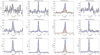 |
Fig. 1 Spectra of sources with H2S detections. The source name, molecular species, and transition are included at the top of each spectrum. The blue lines represent the Gaussian fit to the observed spectra. In the case T Tau, the blue lines represent a fit with two Gaussians, shown as red and green dashed lines. |
 |
Fig. 2 Spectra of sources with no H2S detections. The source name, molecular species, and transition are included at the top of each spectrum. |
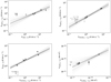 |
Fig. 3 Correlations between line fluxes of the different lines observed. Black dots show the position in the diagrams of detected sources, while gray arrows show the position of upper limits. The dashed black line in each plot depicts a linear fit to logarithmic-scale data. The gray lines show a random selection of 100 models drawn from the obtained posterior distributions. The line fluxes have been normalized to the distance to Taurus (140 pc) to take the dispersion in distances among Taurus members into account. |
Column densities from RADEX assuming a temperature of 20 K and a gas density of 107 cm−3.
Column densities
We used RADEX (van der Tak et al. 2007) to derive molecular column densities assuming a characteristic disk kinetic temperature of 20 K (Williams & Cieza 2011) and a gas density of 107 cm−3. In our first trial, we assumed the beam filling factor to be equal to 1 (i.e., the emission is filling the beam). However, these column densities are lower limits to actual values since no beam dilution was applied. Assuming that most of the emission comes from the disk and assuming a typical disk radius of r = 500 au in T Tauri stars (Pegues et al. 2020; Phuong et al. 2018; Le Gal et al. 2019b), at the distance to Taurus (140 pc; Kenyon et al. 2008) the resulting beam dilution factors are 0.25 for o-H2S, 0.21 for o-H2CO, and 0.20 for CS. If such factors are applied, we derive o-H2S column densities in the range 2.6 × 1012 cm−2 to 1.5 × 1013 cm−2, which are comparable to the column density derived in GG Tau by Phuong et al. (2018) and one to two orders of magnitude larger than the upper limits derived by Dutrey et al. (2011). We note that our estimates of the column densities are based on single-dish observations, while the value derived by Phuong et al. (2018) is based on interferometric observations. As such, the comparison relies on our source size assumption and is subject to large uncertainties. Upper limits derived for o-H2S column densities are in the range 2.6 × 1012 cm−2 to 3.1 × 1012 cm−2, approximately one order of magnitude larger than the upper limits derived by Dutrey et al. (2011).
The resulting column densities are shown in Table 4, and in Fig. 5 we show the column densities of the different species for the sources in the sample computed assuming beam dilution. The Class I sources, GV Tau and HL Tau, show the highest column densities. T Tau shows intermediate values. UY Aur, FS Tau, AA TAu, RY Tau, and DL Tau are Class II sources and show smaller column densities. XZ Tau is a Class II, but the computed column densities arelarger than the other Class II sources in the sample. Contamination from HL Tau may be affecting the measured line fluxes and, subsequently, the column densities. Indeed, as we show in the following section, the computed column densities toward XZ Tau are very close to the values derived for HL Tau. The separation between HL Tau and XZ Tau is 23.05′′, and the beam HPBWs at 168.76 GHz, 150.5 GHz, and 146.97 GHz are 14.2′′, 15.6′′, and 15.8′′, respectively.The contribution from HL Tau to the flux by XZ Tau would be between 0.1% at 168.76 GHz and 0.3% at 146.97 GHz. Therefore, it is unlikely that the fluxes measured toward XZ Tau are due to contamination by HL Tau. High-spatial-resolution observations are needed to resolve this issue.
The derived values depend on the values assumed for the temperature and density. We assumed that the disk is in local thermodynamical equilibrium (LTE) and fixed the density to a value large enough to guarantee LTE conditions (nH= 107 cm−3). To test the impact of changes in the temperature on the derived column densities, we computed the differences with the column densities derived assuming T = 10 K and T = 30 K. The impact of such a change in temperature is small. CS column densities show an average change of 8% when T = 30 K, and of 25% when T = 10 K. The o-H2CO column densities show an average change of 21% when T = 30 K, and of 8% when T = 10 K. Finally, o-H2S column densities change by 4% on average when T = 30 K, and 27% when T = 10 K.
In this section we have assumed that all the molecular emission is coming from the circumstellar disk. This is fully justified for Class II sources that have already dispersed their envelopes. However, this assumption could be more uncertain in the case of Class I sources which still retain an optically thin envelope. In order to gain insight into this problem, we compared interferometric observations of CS and H2CO millimetric lines in Class 0 and I sources (Sakai et al. 2014; Oya et al. 2014; Garufi et al. 2021). While the CS and H2CO emissions present important contributions from the dense envelope in the prototypical Class 0 object L1527 (Sakai et al. 2014), the emission of millimeter lines of CS and H2CO with similarexcitations conditions to those presented in this paper mainly comes from the circumstellar disks in Class I protostars (Garufi et al. 2020, 2021). Therefore, we consider our assumption to be reasonable for our sample.
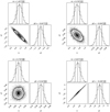 |
Fig. 4 Posterior distributions for the slope (m) and the intercept (y0) for the different correlations explored in the logarithmic space. From left to right and top to bottom: correlations are: H2S vs. CS, H2S vs. H2CO, CS vs. H2CO, and H2S vs. H2O. The verticaldashed lines represent the 16th, 50th, and 84th percentiles. The plots were generated using the PYTHON module CORNER (Foreman-Mackey 2016). |
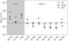 |
Fig. 5 CS, H2CO, and H2S column densities for sources in the sample. We show column densities for GG Tau as well. |
5 Astrochemical modeling
Aiming to understand the observed correlations, we produced a grid of 0D Nautilus (v.1.1) models (Ruaud et al. 2016; Wakelam et al. 2017) that can be compared to our observations. In the following, we summarize the properties of the models and compare the column densities computed in Sect. 4 with the model grid output. Our goal is not to produce a model that fits our data, but rather to synthesize a population that reproduce the observed trends.
5.1 Model grid description
The Nautilus astrochemical code (Semenov et al. 2010; Loison et al. 2014; Wakelam et al. 2014; Reboussin et al. 2015) computesthe evolution of molecular abundances for a given set of elemental initial abundances and physical parameters, including gas and dust temperature, gas density, cosmic ray ionization rate, and extinction. The model includes gas-phase, gas-grain, and surface chemistry reactions. Nautilus (v.1.1) (Ruaud et al. 2016; Wakelam et al. 2017) is a refinement of previous versions that includes both grain surface and grain mantle reactions. A more detailed description of the code is available in Ruaud et al. (2016) and Wakelam et al. (2017).
To compute our models we included both photodesorption and chemical desorption. Our first grid of models consisted of 1600 models that covered a combination of gas densities, gas temperatures, UV flux, and visual extinction. Since the goal of Nautilus (v.1.1) is to follow chemical evolution, it allows for the computation of the molecular abundances at different ages. However, we decided to fix the age to 1 Myr, the value typically assumed for protoplanetary disks in Taurus. A parameter that is known to impact the chemistry of protoplanetary disks is C/O. We computed two different grids using the solar C/O = 0.7 and the carbon rich C/O = 1.0. Since the species of interest are sulfur-bearing, we produced two sets of models: one with solar sulfur abundance ([S/H] = 1.5 × 10⁻⁵) and one with depleted sulfur abundance ([S/H] = 8 × 10⁻⁸). Varying the UV flux and visual extinction only results in larger scatter, without improving our understanding of the underlying correlations, so we decided to fix both parameters and vary the gas density and temperature. We assumed that the dust temperature is the same as the gas temperature. The cosmic ray ionization rate is ζ = 10−17 s−1. A summary of the physical parameters covered by the grid can be found in Table 5. The initial elemental abundances assumed to compute the grid are summarized in Table 6.
Parameters of models in the grid.
Initial elemental abundances for models in the grid.
5.2 Model results
We show in Fig. 6 the comparison of our observations with the grid of models. Since Nautilus does not perform radiative transfer, what we compare is the column density from the models with the column densities derived in Sect. 4. Since the column densities are derived to fit the observed peak intensities, comparing line intensities is equivalent to comparing column densities. And since the derived column densities depend on the assumed source size, the exact position of the observations in these diagrams is subject to uncertainty. However, the shape of the correlation (slope and intercept) will be the same. As can be seen, the models reproduce the correlations, although the slopes and intercepts might differ. Our aim is not to produce a perfect match to the observations, but rather to reproduce the correlation.
The H2S versus H2CO and H2S versus CS models and observations show very similar slopes, while in the case of CS versus H2CO our data points show a slope that is hard to match with the models. The fact that we observe correlations (H2S vs. H2CO and H2S vs. CS) in our small sample arises from the fact that these lines correlate for a large range of physical parameters (Tg and nH). In the case of H2S versus H2CO, the models point to temperatures ranging between 25 and 45 K and densities between 10 and 3 × 107 cm−3. The case of H2S versus CS points to lower temperatures, between 20 and 40 K, and low densities, between 10 and × 106 cm−3. It is interesting to note that the H2S versus H2COC correlation is the one that lasts for a larger range of temperatures and densities. We also note that H2S versus H2CO and H2S versus CS match better with sulfur-depleted models, while CS versus H2CO is better reproduced by models with solar sulfur abundance. The fact that we do not reproduce the CS versus H2CO slope and the need for solar sulfur abundance can both be explained by a lack of proper knowledge regarding the formation and destruction routes for CS. Several theoretical and observational works have pointed out the difficulty in simultaneously explaining the abundances of H2S and CS using a single value of the elemental sulfur abundances and using the current gas and surface chemical networks (Navarro-Almaida et al. 2020; Bulut et al. 2021). Furthermore, CS is an abundant species in different interstellar environments, such as discs, envelopes, and shocks (Snell et al. 1984; Sakai et al. 2016; Oya et al. 2019; Taquet et al. 2020). Minor contributions from different mechanisms might explain this divergence. Regarding the C/O ratio, the comparison of models and observations does not favor either of the two assumed values.
6 Discussion
Our detection of o-H2S in four protoplanetary systems in Taurus comes after its detection in GG Tau by Phuong et al. (2018). Assuming LTE, nH2 = 107 cm−3, Tk = 20K, and a disk size r = 500 au, we derived column densities in the range 2.6 × 1012 cm−2 to 1.5 × 1013 cm−2. This is one order of magnitude larger than the value computed by Phuong et al. (2018) using DiskFit toward GG Tau. In Fig. 5 we show the CS, H2CO, and H2S column densities derived for the disks in our sample together with GG Tau. For GG Tau, we adopted the N(H2S) value from Phuong et al. (2018), while those for CS and H2CO were computed using RADEX to fit the line fluxes provided in Guilloteau et al. (2013). The column densities of all molecules decrease from GV Tau to GG Tau, likely following an evolutionary sequence in which the molecular gas is progressively dispersed from the Class 0 to the Class III stages (only Class I and II sources are present in our sample). The GG Tau H2S column density lies in the region below 1013 cm−2, where we provide upper limits to H2S column densities for AA Tau, DL Tau, and RY Tau. Since there seems to be a hierarchical relation between the column densities, and since our N(CS) upper limits are below the column density for GG Tau, we would expect N(H2S) < 1012 cm−2 for these sources. We note that our estimates of the column densities for CS, H2CO, and H2S are based on a single transition and are therefore subject to large uncertainties. However, an idea of how large these uncertainties are can be obtained by comparing the column densities derived assuming different temperatures. In Sect. 4 we showed that by changing the temperature from 20 to 30 K or to 10 K the column density of H2S changed by 8% and 25% respectively, and therefore we have indications that our estimates of N(H2S) are reliable. It is also interesting to compare the results around these young disks with those in dark clouds. Navarro-Almaida et al. (2020) carried out a detailed study of the H2S chemistry toward the dark cores TMC1-C and Barnard 1b. They found that the H2S abundance is enhanced in the outer part of the envelope, where photodesorption and chemical desorption are most efficient. Our H2S column densities in GV Tau, T Tau, HL Tau, and UY Aur compare well with the values found in the TMC 1 molecular cloud, suggesting that the emission could originate from the surfaces of the cold disk. As mentioned below, this is consistent with our chemical model.
When investigating the chemical evolution of disks, it is interesting to explore the column density ratios that are not affected by differences fluctuations in the total amount of molecular gas throughout the evolution of young stellar objects (YSOs). The column density ratios given in this paragraph were derived from column densities computed assuming beam dilution (see Sect. 4). The sources with a larger N(H2S), namely GV Tau and T Tau, show N(o-H2S)/N(o-H2CO) ratios ~0.5, while those with smaller N(H2S) show a larger N(o-H2S)/N(o-H2CO) ratio of ~0.9. If this is an evolutionary trend, it implies that H2CO is more efficiently depleted onto dust grains compared to H2S in evolved disks. The N(H2S)/N(CS) ratio shows values ranging from 0.12 to 0.38. Carbon sulfide is an ubiquitous species that is very abundant in protostellar envelopes (Sakai et al. 2014, 2016) and molecular outflows (Wolf-Chase et al. 1998; Nilsson et al. 2000; Zhang et al. 2000; Li et al. 2015), and it is not surprising that its column density sharply decreases as the protostellar envelope disappears and the molecular outflow declines. The outflow-envelope component seems less important in o-H2CO and o-H2S. We note that UY Aur is a Class II star, where we do not expect an envelope to be present. To validate the observed evolutionary trends, as well as the tentative correlations, we need a larger sample that allows us to compute reliable statistics.
We identified a possible correlation between the H2S and H2CO lines fluxes that can be explained by the fact that the formation of H2S and H2CO is dominated by surface chemistry reactions, while CS is preferentially formed via gas-phase reactions. It is worth noting that all the stars where we detect H2S belong to multiple systems, and so the role of multiplicity in the chemistry of young protoplanetary systems should be explored. The comparison of the CS and H2S column densities with models seems to favor a large sulfur depletion (S/H = 8 × 10⁻⁸). We note, however, that the sulfur-depleted model overestimates H2CO. N(H2CO) is sensitive to other parameters, such as the initial conditions and the C/O ratio. A detailed exploration of the parameter space is needed in order to understand the chemistry in these systems, to conclude whether there is a large sulfur depletion onto dust grains or not, and to solve this discrepancy.
The sources in the sample were selected because they have been detected through water emission. Eight of them showed water emission at 63 μm (Riviere-Marichalar et al. 2012). We have identified a tentative correlation between the H2O line emission at 63 μm and millimetric H2S emission. According to Riviere-Marichalar et al. (2012), the water emission originated in the inner regions of the disk, from 0.6 to 3 au. If the correlation is real, it would imply that the properties of the inner and the outer disk might be coupled at the early stages of disk evolution.
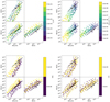 |
Fig. 6 Comparison of the observed correlations with the Nautilus grid of models using two different color codes: Tg (top left), nH (top right), [S∕H] (bottom left), and C/O (bottom right). |
7 Summary and conclusions
Surveying sulfuretted species in protoplanetary disks is key to understanding the evolution of sulfur chemistry during the planet formation stage. In the present paper we show the results of a single-dish survey of the CS 3–2 (f0 = 146.969 GHz), H2CO 21,1 −11,0 (f0 = 150.498 GHz), and H2S 11,0 −10,1 (f0 = 168.763 GHz) lines carried out with the IRAM 30 m telescope. Our main results are the following.
- 1.
We detected CS 3–2 and H2CO 21,1 −11,0 lines toward six out of nine observed sources and H2S 11,0 −10,1 lines toward four of them, namely GV Tau, HL Tau, T Tau, and UY Aur. This adds to the previous detection toward GG Tau, thus increasing the number of H2S detections toward protoplanetary disks from only one to five.
- 2.
We have identified tentative correlations between H2S and H2CO line emission, as well as between H2S and H2O. This could be explained by a common origin of these species on dust grains.
- 3.
Assuming T = 20 K, a gas density of 107 cm−3, and using RADEX, we derived H2S column densities in the range 2.6 × 1012 cm−2 to 1.5 × 1013 cm−2.
- 4.
We used the astrochemical code Nautilus to build a grid of models that can be compared with our observations by varying the gas temperature and density. The grid of models reproduces the observed correlations for a large range of physical conditions.
- 4.
GV Tau shows a particularly low N(H2S)/N(CS) ratio when compared with the rest of the sample, a fact that can be interpreted as an evolutionary effect.
Single-dish observations over a larger sample are needed to confirm our tentative correlations and evolutionary trends. Furthermore, interferometric observations are required to study the spatial distribution of the H2S emission and validate our astrochemical model. Nevertheless, we proposse H2S as a prominent reservoir of sulphur in protoplanetary disks.
Acknowledgements
We thank the Spanish MINECO for funding support from AYA2016-75066-C2-1/2-P and PID2019-106235GB-I100. I.M. is funded by a “Talento” Fellowship (2016-T1/TIC-1890, Comunidad de Madrid, Spain). B.M. is partially funded by the Spanish Ministerio de Ciencia, Innovación y Universidades" through the national project “On the Rocks II” (PGC2018-101950-B-100; PI: E. Villaver).
References
- ALMA Partnership (Brogan, C. L., et al.) 2015, ApJ, 808, L3 [NASA ADS] [CrossRef] [Google Scholar]
- Andre, P., Ward-Thompson, D., & Barsony, M. 1993, ApJ, 406, 122 [Google Scholar]
- Asplund, M., Grevesse, N., Sauval, A. J., & Scott, P. 2009, ARA&A, 47, 481 [NASA ADS] [CrossRef] [Google Scholar]
- Bachiller, R., & Pérez Gutiérrez M. 1997, ApJ, 487, L93 [NASA ADS] [CrossRef] [Google Scholar]
- Baldovin-Saavedra, C., Audard, M., Carmona, A., et al. 2012, A&A, 543, A30 [NASA ADS] [CrossRef] [EDP Sciences] [Google Scholar]
- Balsiger, H., Altwegg, K., Bochsler, P., et al. 2007, Space Sci. Rev., 128, 745 [NASA ADS] [CrossRef] [Google Scholar]
- Bergner, J. B., Guzmán, V. G., Öberg, K. I., Loomis, R. A., & Pegues, J. 2018, ApJ, 857, 69 [Google Scholar]
- Biver, N., Moreno, R., Bockelée-Morvan, D., et al. 2016, A&A, 589, A78 [NASA ADS] [CrossRef] [EDP Sciences] [Google Scholar]
- Boissier, J., Bockelée-Morvan, D., Biver, N., et al. 2007, A&A, 475, 1131 [NASA ADS] [CrossRef] [EDP Sciences] [Google Scholar]
- Boogert, A. C. A., Schutte, W. A., Helmich, F. P., Tielens, A. G. G. M., & Wooden, D. H. 1997, A&A, 317, 929 [NASA ADS] [Google Scholar]
- Booth, A. S., Walsh, C., Kama, M., et al. 2018, A&A, 611, A16 [NASA ADS] [CrossRef] [EDP Sciences] [Google Scholar]
- Bouvier, J., Alencar, S. H. P., Boutelier, T., et al. 2007, A&A, 463, 1017 [NASA ADS] [CrossRef] [EDP Sciences] [Google Scholar]
- Buehrke, T., Brugel, E. W., & Mundt, R. 1986, A&A, 163, 83 [Google Scholar]
- Bulut, N., Roncero, O., Aguado, A., et al. 2021, A&A, 646, A5 [NASA ADS] [CrossRef] [EDP Sciences] [Google Scholar]
- Calmonte, U., Altwegg, K., Balsiger, H., et al. 2016, MNRAS, 462, S253 [CrossRef] [Google Scholar]
- Carr, J. S., & Najita, J. R. 2008, Science, 319, 1504 [NASA ADS] [CrossRef] [PubMed] [Google Scholar]
- Chapillon, E., Dutrey, A., Guilloteau, S., et al. 2012, ApJ, 756, 58 [NASA ADS] [CrossRef] [Google Scholar]
- Codella, C., Podio, L., Garufi, A., et al. 2020, A&A, 644, A120 [CrossRef] [EDP Sciences] [Google Scholar]
- Cox, A. W., Grady, C. A., Hammel, H. B., et al. 2013, ApJ, 762, 40 [NASA ADS] [CrossRef] [Google Scholar]
- Doppmann, G. W., Najita, J. R., & Carr, J. S. 2008, ApJ, 685, 298 [NASA ADS] [CrossRef] [Google Scholar]
- Dutrey, A., Guilloteau, S., & Guelin, M. 1997, A&A, 317, L55 [NASA ADS] [Google Scholar]
- Dutrey, A., Henning, T., Guilloteau, S., et al. 2007, A&A, 464, 615 [NASA ADS] [CrossRef] [EDP Sciences] [Google Scholar]
- Dutrey, A., Wakelam, V., Boehler, Y., et al. 2011, A&A, 535, A104 [NASA ADS] [CrossRef] [EDP Sciences] [Google Scholar]
- Dyck, H. M., Simon, T., & Zuckerman, B. 1982, ApJ, 255, L103 [NASA ADS] [CrossRef] [Google Scholar]
- Edwards, S., Fischer, W., Kwan, J., Hillenbrand, L., & Dupree, A. K. 2003, ApJ, 599, L41 [NASA ADS] [CrossRef] [Google Scholar]
- Edwards, S., Fischer, W., Hillenbrand, L., & Kwan, J. 2006, ApJ, 646, 319 [NASA ADS] [CrossRef] [Google Scholar]
- Foreman-Mackey, D. 2016, J. Open Source Softw., 1, 24 [Google Scholar]
- Foreman-Mackey, D., Hogg, D. W., Lang, D., & Goodman, J. 2013, PASP, 125, 306 [Google Scholar]
- Francis, L., & van der Marel, N. 2020, ApJ, 892, 111 [Google Scholar]
- Fuente, A., Cernicharo, J., & Agúndez, M. 2012, ApJ, 754, L6 [NASA ADS] [CrossRef] [Google Scholar]
- Fuente, A., Treviño-Morales, S. P., Le Gal, R., et al. 2020, MNRAS, 496, 5330 [CrossRef] [Google Scholar]
- Garufi, A., Podio, L., Bacciotti, F., et al. 2019, A&A, 628, A68 [NASA ADS] [CrossRef] [EDP Sciences] [Google Scholar]
- Garufi, A., Podio, L., Codella, C., et al. 2020, A&A, 636, A65 [CrossRef] [EDP Sciences] [Google Scholar]
- Garufi, A., Podio, L., Codella, C., et al. 2021, A&A, 645, A145 [EDP Sciences] [Google Scholar]
- Geballe, T. R., Baas, F., Greenberg, J. M., & Schutte, W. 1985, A&A, 146, L6 [NASA ADS] [Google Scholar]
- Gibb, E. L., & Horne, D. 2013, ApJ, 776, L28 [NASA ADS] [CrossRef] [Google Scholar]
- Gibb, E. L., Van Brunt, K. A., Brittain, S. D., & Rettig, T. W. 2007, ApJ, 660, 1572 [NASA ADS] [CrossRef] [Google Scholar]
- Gibb, E. L., Van Brunt, K. A., Brittain, S. D., & Rettig, T. W. 2008, ApJ, 686, 748 [CrossRef] [Google Scholar]
- Goicoechea, J. R., Pety, J., Gerin, M., et al. 2006, A&A, 456, 565 [NASA ADS] [CrossRef] [EDP Sciences] [Google Scholar]
- Goodman, J., & Weare, J. 2010, Commun. Appl. Math. Comput. Sci., 5, 65 [Google Scholar]
- Guilloteau, S., Piétu, V., Dutrey, A., & Guélin, M. 2006, A&A, 448, L5 [NASA ADS] [CrossRef] [EDP Sciences] [Google Scholar]
- Guilloteau, S., Di Folco, E., Dutrey, A., et al. 2013, A&A, 549, A92 [NASA ADS] [CrossRef] [EDP Sciences] [Google Scholar]
- Hartigan, P., & Kenyon, S. J. 2003, ApJ, 583, 334 [Google Scholar]
- Hartigan, P., Edwards, S., & Ghandour, L. 1995, ApJ, 452, 736 [Google Scholar]
- Herbig, G. H. 1977, ApJ, 214, 747 [NASA ADS] [CrossRef] [Google Scholar]
- Herbig, G. H., & Bell, K. R. 1988, Third Catalog of Emission-Line Stars of the Orion Population : 3 : 1988 [Google Scholar]
- Hirth, G. A., Mundt, R., & Solf, J. 1997, A&AS, 126, 437 [NASA ADS] [CrossRef] [EDP Sciences] [Google Scholar]
- Holdship, J., Jimenez-Serra, I., Viti, S., et al. 2019, ApJ, 878, 64 [NASA ADS] [CrossRef] [Google Scholar]
- Howard, C. D., Sandell, G., Vacca, W. D., et al. 2013, ApJ, 776, 21 [Google Scholar]
- Howk, J. C., Sembach, K. R., & Savage, B. D. 2006, ApJ, 637, 333 [NASA ADS] [CrossRef] [Google Scholar]
- Itoh, Y., Tamura, M., Hayashi, M., et al. 2008, PASJ, 60, 209 [NASA ADS] [Google Scholar]
- Jiménez-Escobar, A., & Muñoz Caro, G. M. 2011, A&A, 536, A91 [NASA ADS] [CrossRef] [EDP Sciences] [Google Scholar]
- Kastner, J. H., Zuckerman, B., Weintraub, D. A., & Forveille, T. 1997, Science, 277, 67 [Google Scholar]
- Kenyon, S. J., Gómez, M., & Whitney, B. A. 2008, Handbook of Star Forming Regions, Low Mass Star Formation in the Taurus-Auriga Clouds, ed. B. Reipurth (USA: ASP Press), 4, 405 [Google Scholar]
- Koresko, C. D. 2000, ApJ, 531, L147 [Google Scholar]
- Kwan, J., & Fischer, W. 2011, MNRAS, 411, 2383 [NASA ADS] [CrossRef] [Google Scholar]
- Laas, J. C., & Caselli, P. 2019, A&A, 624, A108 [CrossRef] [EDP Sciences] [Google Scholar]
- Lada, C. J. 1987, in Star Forming Regions, ed. M. Peimbert & J. Jugaku (USA: ASP Press), 115, 1 [Google Scholar]
- Lada, C. J., & Wilking, B. A. 1984, ApJ, 287, 610 [NASA ADS] [CrossRef] [Google Scholar]
- Le Gal, R., Brady, M. T., Öberg, K. I., Roueff, E., & Le Petit, F. 2019a, ApJ, 886, 86 [CrossRef] [Google Scholar]
- Le Gal, R., Öberg, K. I., Loomis, R. A., Pegues, J., & Bergner, J. B. 2019b, ApJ, 876, 72 [Google Scholar]
- Le Roy, L., Altwegg, K., Balsiger, H., et al. 2015, A&A, 583, A1 [NASA ADS] [CrossRef] [EDP Sciences] [Google Scholar]
- Leinert, C., & Haas, M. 1989, ApJ, 342, L39 [NASA ADS] [CrossRef] [Google Scholar]
- Li, J., Wang, J., Zhu, Q., Zhang, J., & Li, D. 2015, ApJ, 802, 40 [Google Scholar]
- Loison, J.-C., Wakelam, V., Hickson, K. M., Bergeat, A., & Mereau, R. 2014, MNRAS, 437, 930 [NASA ADS] [CrossRef] [Google Scholar]
- Long, F., Herczeg, G. J., Harsono, D., et al. 2019, ApJ, 882, 49 [Google Scholar]
- Long, F., Pinilla, P., Herczeg, G. J., et al. 2020, ApJ, 898, 36 [CrossRef] [Google Scholar]
- Loomis, R. A., Öberg, K. I., Andrews, S. M., & MacGregor, M. A. 2017, ApJ, 840, 23 [Google Scholar]
- Lorenzetti, D. 2005, Space Sci. Rev., 119, 181 [NASA ADS] [CrossRef] [Google Scholar]
- Luhman, K. L., Allen, P. R., Espaillat, C., Hartmann, L., & Calvet, N. 2010, ApJS, 186, 111 [NASA ADS] [CrossRef] [Google Scholar]
- Millar, T. J., & Herbst, E. 1990, A&A, 231, 466 [NASA ADS] [Google Scholar]
- Mumma, M. J., & Charnley, S. B. 2011, ARA&A, 49, 471 [NASA ADS] [CrossRef] [Google Scholar]
- Mundt, R., & Fried, J. W. 1983, ApJ, 274, L83 [NASA ADS] [CrossRef] [Google Scholar]
- Mundt, R., Buehrke, T., Fried, J. W., et al. 1984, A&A, 140, 17 [Google Scholar]
- Mundt, R., Buehrke, T., Solf, J., Ray, T. P., & Raga, A. C. 1990, A&A, 232, 37 [Google Scholar]
- Najita, J. R., Carr, J. S., Brittain, S. D., et al. 2021, ApJ, 908, 171 [CrossRef] [Google Scholar]
- Navarro-Almaida, D., Le Gal, R., Fuente, A., et al. 2020, A&A, 637, A39 [CrossRef] [EDP Sciences] [Google Scholar]
- Nilsson, A., Bergman, P., & Hjalmarson, Å. 2000, A&AS, 144, 441 [CrossRef] [EDP Sciences] [Google Scholar]
- Öberg, K. I., Guzmán, V. V., Furuya, K., et al. 2015, Nature, 520, 198 [Google Scholar]
- Oya, Y., Sakai, N., Sakai, T., et al. 2014, ApJ, 795, 152 [Google Scholar]
- Oya, Y., López-Sepulcre, A., Sakai, N., et al. 2019, ApJ, 881, 112 [Google Scholar]
- Pacheco-Vázquez, S., Fuente, A., Agúndez, M., et al. 2015, A&A, 578, A81 [NASA ADS] [CrossRef] [EDP Sciences] [Google Scholar]
- Palumbo, M. E., Tielens, A. G. G. M., & Tokunaga, A. T. 1995, ApJ, 449, 674 [Google Scholar]
- Pegues, J., Öberg, K. I., Bergner, J. B., et al. 2020, ApJ, 890, 142 [CrossRef] [Google Scholar]
- Phuong, N. T., Chapillon, E., Majumdar, L., et al. 2018, A&A, 616, L5 [NASA ADS] [CrossRef] [EDP Sciences] [Google Scholar]
- Piétu, V., Dutrey, A., & Guilloteau, S. 2007, A&A, 467, 163 [NASA ADS] [CrossRef] [EDP Sciences] [Google Scholar]
- Qi, C., Wilner, D. J., Aikawa, Y., Blake, G. A., & Hogerheijde, M. R. 2008, ApJ, 681, 1396 [NASA ADS] [CrossRef] [Google Scholar]
- Qi, C., Öberg, K. I., Wilner, D. J., & Rosenfeld, K. A. 2013, ApJ, 765, L14 [NASA ADS] [CrossRef] [Google Scholar]
- Reboussin, L., Wakelam, V., Guilloteau, S., Hersant, F., & Dutrey, A. 2015, A&A, 579, A82 [NASA ADS] [CrossRef] [EDP Sciences] [Google Scholar]
- Reipurth, B., Bally, J., & Devine, D. 1997, AJ, 114, 2708 [Google Scholar]
- Riviere-Marichalar, P., Ménard, F., Thi, W. F., et al. 2012, A&A, 538, L3 [NASA ADS] [CrossRef] [EDP Sciences] [Google Scholar]
- Riviere-Marichalar, P., Merín, B., Kamp, I., Eiroa, C., & Montesinos, B. 2016, A&A, 594, A59 [NASA ADS] [CrossRef] [EDP Sciences] [Google Scholar]
- Rodmann, J., Henning, T., Chandler, C. J., Mundy, L. G., & Wilner, D. J. 2006, A&A, 446, 211 [NASA ADS] [CrossRef] [EDP Sciences] [Google Scholar]
- Ruaud, M., Wakelam, V., & Hersant, F. 2016, MNRAS, 459, 3756 [NASA ADS] [CrossRef] [Google Scholar]
- Ruffle, D. P., Hartquist, T. W., Caselli, P., & Williams, D. A. 1999, MNRAS, 306, 691 [Google Scholar]
- Sakai, N., Oya, Y., Sakai, T., et al. 2014, ApJ, 791, L38 [NASA ADS] [CrossRef] [Google Scholar]
- Sakai, N., Oya, Y., López-Sepulcre, A., et al. 2016, ApJ, 820, L34 [Google Scholar]
- Semenov, D., Hersant, F., Wakelam, V., et al. 2010, A&A, 522, A42 [NASA ADS] [CrossRef] [EDP Sciences] [Google Scholar]
- Shingledecker, C. N., Lamberts, T., Laas, J. C., et al. 2020, ApJ, 888, 52 [CrossRef] [Google Scholar]
- Simon, M., Chen, W. P., Howell, R. R., Benson, J. A., & Slowik, D. 1992, ApJ, 384, 212 [NASA ADS] [CrossRef] [Google Scholar]
- Snell, R. L., Mundy, L. G., Goldsmith, P. F., Evans, N. J., I., & Erickson, N. R. 1984, ApJ, 276, 625 [NASA ADS] [CrossRef] [Google Scholar]
- St-Onge, G., & Bastien, P. 2008, ApJ, 674, 1032 [NASA ADS] [CrossRef] [Google Scholar]
- Taquet, V., Codella, C., De Simone, M., et al. 2020, A&A, 637, A63 [CrossRef] [EDP Sciences] [Google Scholar]
- Thi, W. F., van Zadelhoff, G. J., & van Dishoeck, E. F. 2004, A&A, 425, 955 [NASA ADS] [CrossRef] [EDP Sciences] [Google Scholar]
- Tieftrunk, A., Pineau des Forets, G., Schilke, P., & Walmsley, C. M. 1994, A&A, 289, 579 [Google Scholar]
- Uvarova, A. V., Günther, H. M., Principe, D. A., & Schneider, P. C. 2020, AJ, 160, 39 [CrossRef] [Google Scholar]
- van Dishoeck, E. F., Thi, W. F., & van Zadelhoff, G. J. 2003, A&A, 400, L1 [NASA ADS] [CrossRef] [EDP Sciences] [Google Scholar]
- van der Tak, F. F. S., Black, J. H., Schöier, F. L., Jansen, D. J., & van Dishoeck, E. F. 2007, A&A, 468, 627 [NASA ADS] [CrossRef] [EDP Sciences] [Google Scholar]
- Vastel, C., Quénard, D., Le Gal, R., et al. 2018, MNRAS, 478, 5514 [Google Scholar]
- Vidal, T. H. G., Loison, J.-C., Jaziri, A. Y., et al. 2017, MNRAS, 469, 435 [Google Scholar]
- Wakelam, V., Castets, A., Ceccarelli, C., et al. 2004, A&A, 413, 609 [NASA ADS] [CrossRef] [EDP Sciences] [Google Scholar]
- Wakelam, V., Vastel, C., Aikawa, Y., et al. 2014, MNRAS, 445, 2854 [Google Scholar]
- Wakelam, V., Loison, J. C., Mereau, R., & Ruaud, M. 2017, Mol. Astrophys., 6, 22 [NASA ADS] [CrossRef] [EDP Sciences] [Google Scholar]
- White, R. J., & Ghez, A. M. 2001, ApJ, 556, 265 [Google Scholar]
- White, R. J., & Hillenbrand, L. A. 2004, ApJ, 616, 998 [Google Scholar]
- Williams, J. P., & Cieza, L. A. 2011, ARA&A, 49, 67 [NASA ADS] [CrossRef] [Google Scholar]
- Wolf-Chase, G. A., Barsony, M., Wootten, H. A., et al. 1998, ApJ, 501, L193 [NASA ADS] [CrossRef] [Google Scholar]
- Zhang, Q., Ho, P. T. P., & Wright, M. C. H. 2000, AJ, 119, 1345 [NASA ADS] [CrossRef] [Google Scholar]
See http://www.iram.fr/IRAMFR/GILDAS for more information about GILDAS software.
All Tables
Column densities from RADEX assuming a temperature of 20 K and a gas density of 107 cm−3.
All Figures
|
Fig. 1 Spectra of sources with H2S detections. The source name, molecular species, and transition are included at the top of each spectrum. The blue lines represent the Gaussian fit to the observed spectra. In the case T Tau, the blue lines represent a fit with two Gaussians, shown as red and green dashed lines. |
| In the text | |
|
Fig. 2 Spectra of sources with no H2S detections. The source name, molecular species, and transition are included at the top of each spectrum. |
| In the text | |
|
Fig. 3 Correlations between line fluxes of the different lines observed. Black dots show the position in the diagrams of detected sources, while gray arrows show the position of upper limits. The dashed black line in each plot depicts a linear fit to logarithmic-scale data. The gray lines show a random selection of 100 models drawn from the obtained posterior distributions. The line fluxes have been normalized to the distance to Taurus (140 pc) to take the dispersion in distances among Taurus members into account. |
| In the text | |
|
Fig. 4 Posterior distributions for the slope (m) and the intercept (y0) for the different correlations explored in the logarithmic space. From left to right and top to bottom: correlations are: H2S vs. CS, H2S vs. H2CO, CS vs. H2CO, and H2S vs. H2O. The verticaldashed lines represent the 16th, 50th, and 84th percentiles. The plots were generated using the PYTHON module CORNER (Foreman-Mackey 2016). |
| In the text | |
|
Fig. 5 CS, H2CO, and H2S column densities for sources in the sample. We show column densities for GG Tau as well. |
| In the text | |
|
Fig. 6 Comparison of the observed correlations with the Nautilus grid of models using two different color codes: Tg (top left), nH (top right), [S∕H] (bottom left), and C/O (bottom right). |
| In the text | |
Current usage metrics show cumulative count of Article Views (full-text article views including HTML views, PDF and ePub downloads, according to the available data) and Abstracts Views on Vision4Press platform.
Data correspond to usage on the plateform after 2015. The current usage metrics is available 48-96 hours after online publication and is updated daily on week days.
Initial download of the metrics may take a while.